AT-GIS: Highly Parallel Spatial Query Processing with
Associative Transducers
Peter Ogden
Imperial College London [email protected]
David Thomas
Imperial College London [email protected]
Peter Pietzuch
Imperial College London [email protected]
ABSTRACT
Users in many domains, including urban planning, transportation, and environmental science want to execute analytical queries over continuously updated spatial datasets. Current solutions for large-scale spatial query processing either rely on extensions to RDBMS, which entails expensive loading and indexing phases when the data changes, or distributed map/reduce frameworks, running on resource-hungry compute clusters. Both solutions struggle with the sequential bottleneck of parsing complex, hierarchical spatial data formats, which frequently dominates query execution time. Our goal is to fully exploit the parallelism offered by modern multi-core CPUs for parsing and query execution, thus providing the performance of a cluster with the resources of a single machine.
We describe AT-GIS, a highly-parallel spatial query processing system that scales linearly to a large number of CPU cores. AT-GIS integrates the parsing and querying of spatial data using a new computational abstraction calledassociative transducers(ATs). ATs can form a single data-parallel pipeline for computation without requiring the spatial input data to be split into logically independent blocks. Using ATs, AT-GIS can execute, in parallel, spatial query operators on the raw input data in multiple formats, without any pre-processing. On a single 64-core machine, AT-GIS provides 3×
the performance of an 8-node Hadoop cluster with 192 cores for containment queries, and 10×for aggregation queries.
1.
INTRODUCTION
Sources of spatial data are growing at an ever increasing rate. Crowd-sourced projects such as OpenStreetMap [21] create contin-uously-updated, planetary-scale datasets with 100s of millions of objects—the latest weekly OpenStreetMap snapshot is over 40 GBs compressed, 596 GBs uncompressed. High-resolution imaging, from microscopes to satellites, is another source of massive spatial data that can be analysed. In urban planning [5], transportation [52], en-vironmental science [22] and medical image analysis [31], data sci-entists therefore face the task of executing spatial analytics queries over large datasets in an efficient manner. Spatial queries include se-lecting shapes within regions, summarising shapes that meet given criteria, and finding all intersecting or overlapping shapes. From these primitives, more complex queries for testing for shape
sim-ilarity between datasets or determining changes over time can be built.
In domains with new or constantly updated spatial datasets, a key requirement is a lowdata-to-querytime [2], i.e. the time to obtain a query result after the data becomes available. In pathology image analysis, in which segmented image data is queried for anomalous artefacts, it is one of the limiting factors for fast diagnosis [60]; for the OpenStreetMap dataset, this value determines how quickly new geographic features can be incorporated into any analysis.
Currently users who query large spatial datasets must either use relational database management systems (RDBMS) with spatial indexing support, such asPostGIS [25] or Oracle Spatial[45], or employ a distributed compute framework on a cluster, such as
Hadoop-GIS [1] orSpatialHadoop[13]. Both approaches,
how-ever, suffer from a slow data-loading phase, which must occur before spatial queries can be run. RDBMS can only offer fast spatial query processing after the data has been fully parsed, loaded and indexed—in our experiments, loading the complete OpenStreetMap dataset into PostGIS takes over 90 minutes, with an additional 75 minutes to construct the index. Conversely, distributed frame-works with indexing support can offer good query performance, but they require substantially more computational resources than single machine deployments. To spread the load between cluster nodes, they must partition the spatial datasets, e.g. by loading it first into a distributed file system, increasing the total data-to-query time [34]. To reduce the data-to-query time for large spatial datasets, it is paramount to exploit parallelism when parsing, indexing and querying the data. If the original dataset format is simple, as it is the case for the well-known text(WKT) and well-known bi-nary(WKB) spatial formats [42], data-parallelism can be gained from partitioning the input data into independent, fixed-sized blocks and processing them separately [58]—parsing and some spatial filtering can then be performed in parallel, while aggregation and join queries require the combination of all of the data. Unfortunately this simple partitioning approach does not work for more complex, though widely used spatial data formats, including GeoJSON [19] and XML [43]. Due to their hierarchical nature, these formats make it difficult to determine at which boundaries to split the data into independent parts without resynchronising the parser [46].
Our goal is to design a single-machine system for spatial query processing over large datasets that fully exploits the parallelism of modern multi-core CPUs. To minimise data-to-query time, our system should ingest commonly-used source data formats without any pre-processing, following theNoDBphilosophy of executing queries over raw data [2]. The main challenge is that such a system must parallelise the parsing, indexing and spatial query execution. To scale to many CPU cores, it must thus minimise any inter-thread communication or access to global state. While the NoDB philosophy may result in increased I/O bandwidth when the input
data format is complex or queries require multiple data passes, this can be mitigated through on-the-fly indexing and temporary storage. We describe the design and implementation ofAT-GIS, a system for highly-parallel spatial query processing on multi-core CPUs that operates on raw spatial datasets. For containment and aggregation queries, AT-GIS constructs a parallel processing pipeline that parses the data and executes the query in a single pass with constant memory. For spatial join queries, AT-GIS employs two passes, separating parsing and partitioning from the join computation.
To achieve parallelism across many CPU cores, AT-GIS uses a new computational model calledassociative transducers (ATs). ATs allow for the data-parallel execution of otherwise sequential operations, making them a natural model for the processing of complex spatial data formats. With ATs, it is possible to separate parsing, extraction and spatial operator execution into distinct trans-ducers that can be pipelined together. Instead of allocating a thread per transducer, which would limit the degree of parallelism and require synchronisation between them, in ATs each thread executes the entire pipeline, for separate blocks of the input data. Interme-diate results in the pipeline are kept local to each thread, with only the final result synchronised and shared globally.
ATs have two features that enable them to execute multiple de-pendent spatial query processing stages in a data-parallel fashion: (i) they perform some degree ofspeculationduring execution; and (ii) they leverage theassociativityof spatial query operations. Pars-ing, data extraction and spatial operations are performed using finite and pushdown state machines, modified to support out-of-order operation through efficient speculative execution from all possible starting states. A formal model based on transducers allows multiple ATs to be pipelined while maintaining associativity. This permits AT-GIS to implement complex spatial operators using associative algorithms so that partial results can be merged.
We show experimentally that AT-GIS operates efficiently on mul-tiple data formats: it performs spatial aggregation queries on GeoJ-SON or WKT-formatted OpenStreetMap data 2×faster than Spa-tialHadoop on the same hardware, despite not using an index; it is 10×faster than an 8-node Hadoop-GIS cluster, which has 3×the CPU cores and already pre-partitioned data. For spatial join queries, the time that AT-GIS requires to read and partition the dataset in parallel is less than 20% of the time taken to execute the join, with the total query time comparable to that of a larger cluster-based system. AT-GIS also achieves similar query performance, but with a much lower data-to-query time, as a commercial parallel DBMS with indexing for containment and aggregation queries and shows a two orders-of-magitude improvement over PostGIS.
The rest of paper is structured as follows: §2 discusses the prob-lem and existing solutions for spatial query processing over large datasets; §3 describes the model of associative transducers for spa-tial queries; §4 presents the design of AT-GIS, explaining its query processing stages; §5 evaluates our prototype implementation; §6 discusses related work; and §7 concludes.
2.
SPATIAL QUERY PROCESSING
We now introduce spatial queries (§2.1) and the challenges when querying large datasets (§2.2). We then discuss two approaches for large-scale spatial query processing (§2.3): spatial extensions to RDBMS and distributed systems based on the map/reduce model.
2.1
Spatial queries
As the size of data has increased, so has data that incorporates a spatial component [33]. Given that spatial searching is widely used in modern web applications [12], a common use of spatial data is in relating places on the surface of the earth. Other uses for geospatial processing are finding correlations between datasets acquired from
Listing 1: Example fragment of GeoJSON file 1 { " type ": " F e a t u r e C o l l e c t i o n ", 2 " f e a t u r e s ": [ 3 { " type ": " F e a t u r e ", 4 " g e o m e t r y ": { 5 " type ": " G e o m e t r y C o l l e c t i o n ", 6 " g e o m e t r i e s ": [ 7 { " type ": " G e o m e t r y C o l l e c t i o n ", 8 " g e o m e t r i e s ": [/* Sha pe Data */] }, 9 { " type ": " L i n e S t r i n g ", 10 " c o o r d i n a t e s ": [ [1.1, 0.0],[1.2, 1.0] ] } 11 ] } 12 " id ": 1 2 3 4, 13 " p r o p e r t i e s ": { /* User Data */ } 14 } 15 ] 16 }
different sources—a key component of current geospatial datastore benchmarks [16, 51]. As well as geospatial data, there is a growing use of spatial analytics in medical imaging, in particular pathology, in order to automate the process of finding a diagnosis from high-resolution digital microscopy images [31].
In this paper, we consider spatial datasets as collections of
ob-jects. Each object consists of ageometry, as defined by the Open
Geospatial Consortium Standard [42], and associated metadata. Supported types of geometries are linestrings, polygons, multipoly-gons and collections. An example of a dataset consisting of one object is given in Listing 1. Here the geometry is a collection, and the metadata is both an identifier and user-provided properties.
We focus is on three classes of spatial queries:
Containment queriesare the most basic primitive in spatial pro-cessing and perform a filtering operation on the data. The canonical example is finding all geometries contained within a region, but any filtering query against a defined set of reference objects can be considered as containment.
Aggregation queriesare an extension of containment queries and involve some summarisation over the filtered result set. The sum-mary can be numeric, such as the average area of all selected ge-ometries, or spatial, e.g. computing the set-spatial union of all shapes in the set. Multiple aggregations can also be performed simultaneously, as done byGROUP BYSQL statements.
Join queriesare one of the most expensive operations associated with spatial querying because, in the worst case, every geometry in one dataset must be compared with every geometry in another. To reduce the number of pairs of geometries for comparison and to parallelise the computation, it is common to divide the shapes into
spatial partitions[48, 24]. Each partition contains a subset of the
dataset within some defined area, and disjoint partitions can thus be processed in parallel. Partitioning allows join processing to scale to multiple CPU cores, but introduces an additional partitioning step.
2.2
Scalability challenges
The wide availability of always-connected, location-aware mo-bile devices is causing a massive growth in the quantity of spatial data being generated and stored [63, 61]. Crowd-sourced mapping and behavioural data has become mainstream for uses such as navi-gation [21] and epidemiology [23], with the number of users con-tinuing to grow. Standards are already being developed to support the next generation of sensor and IoT systems in which updates will be continuously streamed [7], thus requiring spatial data processing systems to operate without prior offline data partitioning.
Since CPU clock speeds have remained relatively constant, multi-core processing is essential for achieving fast query results [57]. For a lowdata-to-query time, all query processing stages must be parallelised. Most data querying systems now implement some form of parallelism once the data is loaded; few systems, however,
consider how data can be loaded in parallel. Loading data in parallel requires the concurrent execution of two operations:parsingthe source data format andpartitioningorindexing. When the data on disk is not spatially partitioned, distributing the parsing in cluster systems causes significant I/O load as geometries are shuffled from the node responsible for parsing to the nodes with the correct spatial partitions [47]. The same is true when loading data in parallel into a single-node sharded database: here network I/O is replaced by disk I/O when moving geometries to the correct database instance.
Following a NoDB philosophy [2], a scalable spatial querying system should support the input data efficiently no matter what its format is. Many existing formats for spatial data, however, are complex to split and parse. RDBMS with spatial extensions usually handlewell-known text(WKT) andwell-known binary(WKB) [42] geometries contained inside comma or tab separated files. This makes splitting the data a case of searching for newlines in the dataset. Public spatial datasets, however, tend to favour more struc-tured data formats, such as XML [43] and JSON [8], in order to simplify interoperability. These semi-structured formats do not have the same ease of splitting as database bulk formats.
As a result, we focus onGeoJSON[19] because it encompasses many features that make parallel processing challenging, such as a recursive definition and support for arbitrary metadata. An example fragment is given in Listing 1. Allowing geometries to contain other geometries prevents splitting based on hierarchy; supporting free-form user metadata makes splitting using known strings unsound— without full parsing, it is impossible to decide if the string indicates a hierarchy boundary or is part of the metadata. We also consider WKT- and XML-formatted data to show the flexibility of our ap-proach in handling different input formats.
2.3
Existing solutions
Spatial DBMS.Both relational and NoSQL-style database engines have added spatial query support: Oracle[45], Microsoft
SQL-Server[15] andIBM DB2[9] all offer spatial extensions, as well
as several open-source engines, includingPostGIS[25] and My-SQL[39]. RDBMS support spatial data through the use of spatial indexes, such asR-trees[40] (used by PostGIS) orQuadtrees[32] (available in Oracle). These index structures operate on the bound-ing boxes of geometries, providbound-ing an efficient mechanism to select possible matches. Each possible match still needs to be refined by comparing the geometries, a process often taking longer than the index search [54]. There is also the upfront cost of creating the index, which may dominate for regularly updated datasets.
In contrast, the MonetDBcolumn store [59] does not have a spatial index but instead stores bounding boxes as a separate col-umn [38]. The rationale is that the sequential access pattern of scanning a column offsets the extra computation due to the lack of an index. MonetDB can parallelise some operations, but spatial joins are sequential and require constructing the entire candidate set in memory. For containment queries, sequentially laid-out bounding boxes can achieve performance comparable to indexes for pfiltering. This approach fails to scale to large joins because it re-quires sufficient memory to hold the product of the joined columns.
GeoCouch[18] supports simple filtering primitives for the
Couch-DB NoSQL datastore [3]. There is no join support, and the perfor-mance has so far been shown to be up to 3×worse than PostGIS on a single node [37]. By sharding documents across nodes, it may be possible for GeoCouch to scale, but this has yet to be demonstrated for geospatial data. GeoCouch also has the fewest supported spatial query operators of any of the discussed systems.
Distributed frameworks.The two main implementations for spa-tial query processing on clusters areHadoop-GIS[1] and
Spatial-Hadoop[13], which are both based on the Hadoop map/reduce
framework [10]. While both systems perform data indexing, Hadoop-GIS assumes that index creation is inexpensive and thus can be done mostly on demand, with only the largest regions indexed statically. while SpatialHadoop is more concerned with up-front indexing. Despite the indexing support of these systems, we show that AT-GIS achieves substantially better performance without prior indexing.
Any system built on top of Hadoop requires that the data is first loaded into the HDFS distributed file system with suitable parti-tioning. Both systems use spatial partitioning to distribute objects between nodes. Given that an object can be part of multiple spatial partitions, each system must have a way to either eliminate dupli-cate objects or transfer them between nodes: Hadoop-GIS spends substantial time on boundary handling—objects are duplicated prior to parallel processing and then duplicate results are pruned; Spatial-Hadoop uses more sophisticated indexing structures to avoid this in most cases. While AT-GIS supports partitions similar to Hadoop-GIS, following apartition-based spatial merge joinstrategy [48], its single-node design eliminates expensive network I/O.
Discussion.All of the above approaches for spatial query process-ing require that the input data is loaded first so that indexprocess-ing or partitioning can be performed. Once loaded, the data is processed in parallel using the internal data structures to create independent work units. An important requirement for a system with a low data-to-query time, however, is that it operates in parallel from the start, without assuming the existence of any ancillary data structures.
A related requirement is for the data to be left in its original form. A conversion of data into an internal representation requires at least two data passes: one pass to do the conversion, and a second pass to perform the query. For loaded data, a more compact representation may be used, which reduces I/O bandwidth for queries such as joins that require multiple passes of the data on disk; for single-pass queries, however, this may increase I/O bandwidth usage.
Finally, the system should operate on a single node in parallel. For current map/reduce-based cluster systems, significant inter-node communication is necessary during the reduce phase to handle geometries that straddle partition boundaries. By confining compu-tation to a single multi-core node, this deduplication can be handled internally rather than being limited by the network bandwidth.
3.
ASSOCIATIVE TRANSDUCERS
To execute spatial queries with a single data pass, we need a computational model that is expressive enough to represent the whole processing pipeline for spatial queries, from the parsing of the raw spatial data to the execution of spatial operators. The model must also be parallelisable and should have bounded internal state. Whiletransducers[36] have primarily been used for lexing and parsing, we introduce a new transducer class, called associative
transducers, that can express a wide range of spatial query
opera-tions. Transducers are an inherently sequential model, but we show that, through a combination ofspeculation[41] and the properties of our new transducer class, it becomes possible to construct pipelines of transducers that can execute spatial queries with data parallelism. First we provide a formal description of associative transducers and show how they support data-parallel operations (§3.1) while maintaining the property of compositionality required to construct complex spatial query processing pipelines (§3.2). After that, we discuss the specific types of transducers needed to support spatial querying (§3.3) and how they map to spatial query operators (§3.4). Finally, we introducepartially-associative transducers, an optimi-sation that reduces the overhead of speculation (§3.5).
3.1
Formal description
We assume a transducerT can be represented as a five-tuple T = (Q,q0,Σ,Γ,δ)whereQis the set of states,q0is the starting
1 start 2 3 a b a b /∗ a b
Figure 1: Transducer for matching the stringab
state,Σis the input alphabet,Γis the output alphabet, andδ is
the transition function. We only consider deterministic transducers, makingδa function of the current state and input symbol. We do not require thatQis finite to ensure that the model can express both aggregations across infinite sets and pushdown transducers.
If we combine the stateQand output tapeΓ∗of a regular trans-ducer into a pairp∈P= (Q×Γ∗), we can think of execution as
an operatorps→p0wheresis an input symbol.is defined as performing the state transition ofT and updating the output tape. The result of processingT on a string of symbolss1,s2,· · ·,siis
the same asp0s1s2· · · siwhere p0= (q0,ε).is clearly non-associative because it cannot operate on two symbols, relying on a left-reduction to be well-formed.
Anassociative transducer(AT), denoted asT0, is a generic con-struction overT to support associative operations. We wish to be able to define a function⊗that has the same semantics asbut supports associative reduction. We define ATs as havingfragments, rather than states. A fragmentf0contains astate mapping relation q0∈Q0:[Q→Q]that maps potential starting states to correspond-ing finishcorrespond-ing states, whereQ0 is the set of all such relations. A fragment also contains a set of predicated output tapeso0∈[Q→Γ∗]
to store the symbols emitted by the transducer. The predicates are needed because some output symbols may only be emitted for a subset of possible starting states.
The state mapping relation begins as the identity relation. As symbols are processed, each entry in the fragment has its finishing state updated. Merging two fragments results in the composition of the two relations. As the composition of relations is associative, the action of the AT is also associative.
Using these definitions, we can now define an operator:
(q0,o0)si→ {(qi,q∗) |(qi,qf)∈q0andq∗=δQ(qf,si)}, {(qi,o:o∗)|(qi,o)∈o0and(qi,qf)∈q0and o=δΓ(qf,si)}
where : is string concatenation, andδQandδΓare defined such that
δ(q,si) = (δQ(q,si),δΓ(q,si)).
We now transform each symbol in the input into a fragment independently. We also define a function⊗to merge fragments:
(q01,o01)⊗(q02,o02)→ q01◦q02, {(qs,o1:o2)|(qs,o1)∈o01and (qs,o2)∈q◦o02}
where◦is relation composition. As this function depends only on relation composition and string concatenation, which are both asso-ciative operations, the resulting merge function is also assoasso-ciative.
Rather than two relations, the fragment can be considered equiva-lently as afragment function, which takes a starting state and returns the corresponding finishing state and output tape. Using this model, we can find efficient ways to represent the fragment function other than storing the relations directly (see §3.3).
Example (Matching transducer): Consider the simple string
trans-ducer in Fig. 1 that outputs*each time the stringabis seen. To operate on the stringabab, we split the string into individual sym-bols and construct execution pairs for each one:
Input a b a b
Fragment {1,2,3} →2 {1{,3} →1 {1,2,3} →2 {1,3} →1
2} →3 {2} →3
Output {2} → ∗ {2} → ∗
The symbolbresults in an execution pair that outputs a single*if the actual starting state turns out to be 2, but not if the starting state was 1 or 3. The next step is to combine the pairs associatively:
Input ab ab
Fragment {1,2,3} →3 {1,2,3} →3 Output {1,2,3} → ∗ {1,2,3} → ∗
These intermediate results show the property ofconvergence: the number of distinct finishing states in the relation decreases as data is processed. Since the transducer is deterministic, the number of distinct finishing states in a fragment cannot increase.
The final step is to merge the remaining two execution pairs to compute that, regardless of the starting state, the finishing state is 3, with**on the output tape.
3.2
Composition and parallel execution
By storing fragments for the next transducer in a pipeline, rather than the output tape, we can compose multiple ATs. We observe that the string concatenation operator : can be replaced by any as-sociative operator⊗without invalidating the transformation. When two ATs are combined, the first transducer now stores a predicated set of fragments from the second transducer, rather than the output tapes. This model can be extended to a pipeline of arbitrary length. One possible way of parallelising a pipeline would be to exe-cute each stage concurrently, but this would limit the degree of parallelism to the number of transducers in the pipeline and require synchronisation to pass data between them. Instead, the pipeline can be executed in adata-parallelfashion, constructing fragments independently for blocks of data that can then be merged together. This provides greater parallelism, which is better suited to achieve scalable query processing with many CPU cores.
Example (Counting transducer): Building on the previous example,
to count the number of*symbols on the tape, we can construct a simple counting transducer withQ=N, which increments when a *is seen as input. We then compose the two transducers to count the occurrences ofab. Using the same string and the matching transducer as before, we can see below that, underb, a 1 is contained in the predicated list and a 0, otherwise.
Input a b a b
Fragment {1,2,3} →2 {1{,23} →} →13 {1,2,3} →2 {1{,32} →} →13 Output {1,2,3} →0 {1{,23} →} →01 {1,2,3} →0 {1{,32} →} →01 The execution proceeds analogously to the previous example except that, instead of concatenation, we add the fragments of the counting transducer. The result is that, regardless of the starting state, the fin-ishing state of the matching transducer is 3, with 2 as the fragment of the counting transducer.
3.3
Spatial query processing
Next we explore efficient implementations of the fragment func-tion for different types of transducers needed for spatial query processing. We identify five types of ATs that can be mapped to operations when processing spatial data:
1. finite state transducersfor lexing the input data;
2. deterministic pushdown transducersfor extracting the data and
metadata from lexed symbols;
3. stateless transducersfor conversions on points or aggregates;
4. aggregation transducersfor summarising data; and
5. periodically flushing transducersfor aggregating geometries.
We look at each in turn, grouping the conceptually similar finite and pushdown transducers together along with the stateless and aggregation transducers. To illustrate the use for each type of
trans-1 start 2 3 4 5 6 7 8 9 10 11 12 13 14 15 16 Linestring[ [ ] ] Polygon[ [ [ ] ] ] Multpolygon[ [ [ [ ] ] ] ]
(a) Deterministic transducer
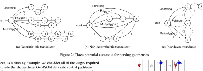
1 start 2 4 5 6 7 Linestring[ Multipolygon[ Polygon[ [ [ ] ] ] ] ] (b) Non-deterministic transducer 1 start 2 3 4 5 Linestring[ [ ] ] Polygon[ [ ] ] Multpolygon[ [ ] ] (c) Pushdown transducer Figure 2: Three potential automata for parsing geometries
ducer, as a running example, we consider all of the stages required to divide the shapes from GeoJSON data into spatial partitions.
Finite and pushdown transducerscan extract spatial data from a raw format. Finite transducers have an explicit associative form: each fragment contains the state mapping relation from all possible starting states to the corresponding finishing states and a set of out-put tapes predicated by the starting states. When an inout-put symbol is processed, each entry in the relation is updated, and output symbols are appended to the output tapes.
A natural way to express these relations are asN×N binary matrices, whereNis the number of states in the transducer. For a small number of states, the transitive closure under multiplication can be precomputed as a set of lookup tables. This is similar to the approach used bysimultaneous finite automata[56] but with the addition of an output tape.
Each output tape in the fragment has a predicated set of start-ing states represented by a vector. By considerstart-ing all output tapes formed as a vector, a matrix can be used to associate starting states with corresponding output states. The complete fragment thus holds a state relation mapping matrix, an output matrix and a vector of output tapes. This representation allows for tapes to be shared among multiple starting states after convergence was achieved.
All of the relation composition operations needed to merge exe-cution pairs thus become precomputed matrix multiplications. Merg-ing the output tapes from each pair thus becomes the dominant fac-tor in performing merges. This is mitigated by limiting the number of possible starting states based on the structure of the lexer. For example, in XML, it can be guaranteed that if a block starts with a <character, there are only three possible starting states (comment, CDATAor neither); the,character in JSON can fulfil a similar pur-pose. This can only be done without impacting performance if the searched character is common in the input stream [41].
It is possible for the same parsing task to be implemented using different automata models. Fig. 2 shows the transition diagrams of parsers for a simplified geometry format based on GeoJSON. A deterministic finite transducer requires fewer states than either a non-deterministic or a pushdown transducer (Fig. 2a). As the cost of speculation depends on the number of states, and we do not have a formal model for a non-deterministic transducer (Fig. 2b), we choose to implement the parsing of spatial data formats using pushdown transducers (Fig. 2c).
Stateless and aggregation transducers.The stateless (SLT) and aggregation (AGT) families of transducers correspond to the func-tionalmap/filterandreduceprimitives found in parallel process-ing [10, 26]. They are used to support mathematical and spatial transformations and aggregations in spatial queries. We exploit their associativity to provide efficient AT implementations.
A stateless transducer is one for which the set of statesQis a singleton⊥, i.e. there is no shared state carried over between input symbols, and each can be processed independently. The transition
1 1
2 2 1,2 2
1
⊗ →
Figure 3: Partitioning expressed as an associative operation functionδthus takes the formδ(⊥,s)→(⊥,p(s))wherep:Σ→ Γ∗is the mapping function. Each input can result in zero or more outputs, giving it the expressive power of bothmapandfilter. A stateless transducer has a trivial associative form without any state to manage. For example, coordinate space conversion—a common operation in spatial querying—can be done by stateless transducers.
Example (Point parser): A point parser is a transducer that takes
streams of point offsets and produces a stream of point values. It is used to isolate the structural parsing, performed by finite and push-down transducers, from handling floating point values. It is stateless as each offset can be parsed into a point value independently, with no dependencies between adjacent symbols in the input data.
Aggregation transducers perform some reduction over the input data without producing output. The reduction function combines the internal state of the transducer with the input value to produce the new internal state. More formally, an aggregation transducer has a transition functionδ(q,s)→(a(q,t(s)),ε)where the
transforma-tion functransforma-tion t:Σ→Qconverts each input symbol into a state, and
anaggregation function a:Q×Q→Qcombines states.
An efficient AT relies on the properties of the aggregation func-tion: if the function is associative, the transformation only needs to store one copy of the in-order state to reconstruct the whole state relation. If the aggregation function is not associative, another approach is needed, typically buffering until the aggregation can be run in-order. Aggregations can be numeric, e.g. when computing the sum of values, or spatial, e.g. when computing the set-theoretic union of a list of shapes.
Example (Partition): Spatial partitioning is an example of an
op-eration that can be performed by an aggregation transducer. The state of the transducer contains a set of spatial partitions and the identifiers of the contained objects. Fig. 3 shows two partitions, each containing a single object numbered 1 and 2. The associative merge operation (⊗) concatenates the list of objects in each partition.
Periodically flushing transducersare a hybrid of stateless and ag-gregation transducers and can perform agag-gregations over subsets of the input stream, e.g. computing a bounding box for each geometry. The set of input symbols can be divided into two disjoint sets: P for processing symbols and F for flushing symbols. When a flushing symbol is received, zero or more output symbols are emit-ted, and the internal state resets to the starting stateq0; when a processing symbol is received, the internal state is updated but no symbols are output. Thus periodically flushing transducers perform aggregations on strings of processing symbols demarcated by flush-ing symbols. The processflush-ing symbols are typically points or edges, and the flushing symbols are markers for geometry boundaries.
P P P F P P P P F P P P F P P
F Flushing symbol P Processing symbol P Complete geometry
Speculative Main
Processing state:
Symbol stream: Main reset after each geometry
Figure 4: Data processing with a periodically flushing transducer As with aggregation transducers, the most efficient transforma-tions into an associative form arise when the aggregation function is itself associative. In this case, the fragment of an AT can be represented using two copies of the in-order state: thespeculative andmainstates. Fig. 4 shows the speculative state that is used to aggregate the processing symbols before the first flushing symbol, while the main state is used for all input symbols from that point on. An additional bit is needed to record if at least one flushing symbol was seen and hence which copy of the state should be used for processing the next input symbol. Only one output tape is needed to store the results of the main state. The output from the speculative state is not determined until merging.
To merge two associative fragments, the main state at the end of the first must be merged with the speculative state at the beginning of the second. The result is a new aggregation that must be inserted into the output tape between the tapes of the two merged fragments.
Example (Polygon bounding): A periodically flushing transducer
can compute the master bounding rectangles (MBRs) of geometries. The processing symbols are the point values, and the flushing sym-bols are the special values marking the boundaries of geometries. MBR computation from a list of points is an associative operation as each point can be considered as its own bounding box, and an associative operation computes the union of the boxes. Merging can similarly be performed by computing the spatial union of the two partial states being merged.
3.4
Support for spatial operators
Next we consider a set of spatial operators and describe how each can be expressed as an AT. We first explain the case in which operators are used as a predicate with a single or small set of objects provided as a query parameter, and then describe how the operators can be used for joins. Finally, we address extensions, as used by PostGIS and other spatial DBMS, to provide geometry aggregation. We focus on the spatial operators provided by the SQL option of theOpen Geospatial Consortium Simple Feature Access
Spec-ification[42] when comparing polygons to polygons, as listed in
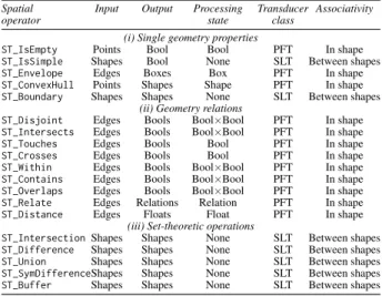
Table 1. We split the operators into three categories: operators that (i) calculate some property on a single geometry; (ii) spatially relate two geometries; and (iii) represent set-theoretic operations on one or more geometries. Table 1 shows the mapping into transducers when one of the operands is a query parameter. We consider the case in which operators are used in a join query separately.
For each operator, we state the input and output types of the cor-responding transducer as well as the type of any internal state. The class of each generated transducer (from §3.3) is also listed along with the corresponding associativity available. The most flexible form of associativity is “in shape”, which allows a single shape to be distributed; “between shapes” requires that each shape is allocated to a single thread, potentially reducing parallelism.
The first category of operators contains those that operate on a single geometry to perform some form of aggregation. With the exception ofST_IsSimpleandST_Boundary, both of which must consider the geometry in its entirety, the others can be implemented as PFTs, constructing a partial aggregation and merging the two. We have already explored the case of bounding box calculation as part of the running example in the previous section.
Spatial Input Output Processing Transducer Associativity operator state class
(i) Single geometry properties
ST_IsEmpty Points Bool Bool PFT In shape
ST_IsSimple Shapes Bool None SLT Between shapes
ST_Envelope Edges Boxes Box PFT In shape
ST_ConvexHull Points Shapes Shape PFT In shape ST_Boundary Shapes Shapes None SLT Between shapes
(ii) Geometry relations
ST_Disjoint Edges Bools Bool×Bool PFT In shape ST_Intersects Edges Bools Bool×Bool PFT In shape
ST_Touches Edges Bools Bool PFT In shape
ST_Crosses Edges Bools Bool PFT In shape
ST_Within Edges Bools Bool×Bool PFT In shape ST_Contains Edges Bools Bool×Bool PFT In shape ST_Overlaps Edges Bools Bool×Bool PFT In shape ST_Relate Edges Relations Relation PFT In shape ST_Distance Edges Floats Float PFT In shape
(iii) Set-theoretic operations
ST_IntersectionShapes Shapes None SLT Between shapes ST_Difference Shapes Shapes None SLT Between shapes ST_Union Shapes Shapes None SLT Between shapes ST_SymDifferenceShapes Shapes None SLT Between shapes ST_Buffer Shapes Shapes None SLT Between shapes
Table 1: Representation of spatial operators as ATs The second category includes all those operations that perform some spatial relation. When comparing against a known reference set, these operators can be executed using an algorithm that com-pares each edge in turn. UsingST_Intersectsas an example, we use an edge testing algorithm that compares each incoming edge with the edges in the reference set. Any crossing means that the geometry intersects with the reference. To handle the case in which one polygon is entirely inside another, we perform two point-in-polygon tests, one comparing the first point in the geometry against the reference set and the second comparing an arbitrary point in the reference set against the geometry. If either of these two tests matches, the geometries are intersecting.
The final category includes set-theoretic operations on shapes. As such operations require processing the entire polygon as a single en-tity rather than each point or edge individually, we cannot use a PFT. Instead we use transducers that operate on a stream of polygons as stateless transducers when each operation is independent, e.g. using ST_Bufferon a stream orST_Differenceon a stream of joined pairs or with a reference object. Alternatively, when the operator is used as an aggregation across a column, e.g. usingST_Unionon a large set of geometries, we can take advantage of the associativity of set operations to use an aggregation transducer.
When a spatial predicate is used for a join between two large sets of geometries, the model used for a small reference set ceases to be effective, requiring an alternative approach. Typically some version of a plane or line-sweep algorithm can be used. Our transducer model is not a good fit for a join between two data streams, so we wrap the join into a transducer that takes sets of shapes as input and emits joined pairs as the output stream. This permits the use of transducer operations before and after the join, while having the performance of existing parallel joins. We use apartition-based
spatial merge join[48] to perform all spatial joins between two
datasets, using transducers for the initial partitioning.
3.5
Partially associative transducers
Depending on the input data, it may be possible to relax the requirement for full associativity to reduce speculation.
Partially-associative transducersare an optimisation when the data can be
split in such a way that the state at the start of a block is known. This is common in many spatial data formats, even recursive ones such as GeoJSON, if the complete schema is known in advance.
The idea for this optimisation is to introduce some logic into the splitting of the data into blocks such that block boundaries occur only at locations that result in known states: in comma- or tab-separated text files with no escaping, this is typically the end of
Data file Pipelines Pipelines Pipelines Pipelines Pipelines Pipelines Final result Split phase Processing phase Merge phase
Figure 5: Phases of pipeline execution in AT-GIS lines; in XML or JSON, it is commonly some tag that only appears at a given point in the hierarchy and that can be used to establish the state of the parser for the block.
In some cases, it may be possible for the tag to appear at an unexpected location due to a free-form field in the input. A partially-associative transducer may then temporarily process the data incor-rectly, but the inconsistency will be caught during a subsequent merge. The data would then have to be reprocessed, but it would not affect the correctness of the final result.
Example (GeoJSON parsing): For GeoJSON, the parse and
query-ing stages can be converted into a partially-associative form by exploiting the object type field that appears within each object. If object boundaries can be found, the lexer and parser can be started in a known state, permitting the use of an optimised, off-the-shelf library without speculation. For example, it is possible to use a regular expression to search for the string"type":"Feature", as seen on line 3 in Listing 1. Since the tag is not necessarily the start of an object, a parser can find the boundaries of the object.
4.
AT-GIS DESIGN
In this section, we describe how AT-GIS uses associative trans-ducers (ATs) to create parallel processing pipelines for the execution of spatial queries. First we introduce its processing model (§4.1) and present the pipelines for different query types (§4.2), explaining their physical query plans, how stages are decomposed into ATs and how the system is implemented (§4.3). After that, we focus on each pipeline stage in turn, exploring the trade-offs for performance optimisation (§4.4). We finish with a discussion of spatial joins and how they use multiple pipelines (§4.5).
4.1
Overview
AT-GIS executes spatial queries by translating aphysical query
planintopipelinesof transducers. The physical plan takes the form
of a dataflow representation of the query [53] in which the majority of spatial operators are compiled into a single pipeline. Joins require multiple pipelines because they rely on barriers.
The construction of the physical query plan follows past work on optimising pipelined parallel query execution [6]. AT-GIS as-sumes a tree-shaped dataflow graph in which each spatial operator is represented by a node; edges denote the objects transfered be-tween operators. AT-GIS supports a hierarchy of four object types,
withpointsbeing the lowest level, followed byedges,ringsand
polygons. In general, edges should be typed with the lowest-level
object supported by both sides—the lower the level, the greater the opportunity for parallelism. All but conditional and join operators have a single input and output edge.
AT-GIS then constructs a pipeline from each linear section of the dataflow graph. It makes special consideration for conditional operators (§4.4.2) to allow them to form part of a linear pipeline in spite of them not being linear. Once the pipelines have been defined, AT-GIS compiles them using an optimising compiler to reduce the overhead of the abstraction between stages.
As shown in Fig. 5, the execution of pipelines involves three
phases:split,processing andmerge. The split phase divides the
input data into blocks. Data splitting may require incrementing a pointer (for fully-associative transducers) or executing a regular expression and lightweight parsing (for partially-associative
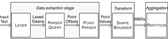
trans-LEXER PARSER QUERY POINT PARSER SHAPE BOUNDER PARTITION Data extraction stage Transform Aggregation Input Text Lexed Tokens Point Offsets Point Values MBRs
Figure 6: Pipeline for shape partitioning in a textual data format ducers). After a data block is formed, it is placed in a work queue for the processing phase. The processing phase performs the majority of the computation by passing blocks from the work queue through the pipeline. As ATs make the tasks independent, it can be scaled to many parallel threads. The merge phase combines all of the partial results from the processing phase to compute the final query result. While the first two phases can run concurrently to reduce latency, the third phase executes only after all blocks are available.
4.2
Spatial query processing pipelines
Fig. 6 shows how a single-pass pipeline can be split into three logicalstages: (i) parsing of the dataset and extracting the data of interest; (ii) transforming and filtering the data to answer the query; and (iii) aggregating the result. Theparsing/data extractionstage is responsible for consuming bytes from the input file and outputting a stream of point values. If required by the query, any filtering on the metadata is also handled by this stage. Restricting metadata queries to the first stage ensures that format-specific knowledge is not needed in the rest of the pipeline. The
transformation/fil-tering stage encompasses any operations that process individual
geometries or points and consists primarily of periodically flushing transducers. Finally, theaggregationstage performs any aggrega-tion across all the geometries. In the case of a containment query, the final stage buffers the result for output.
Each object between pipeline stages is tagged with the data offset from which it was created. Offsets are used in two ways: to enable unique identification of points and geometries; and to allow re-parsing of objects in the join pipeline. The type of the objects transfered between the transformation and aggregation stage de-pends on the nature of the aggregation: spatial aggregations require that the aggregation stage receives all point data, whereas numeric aggregations require only the computed result.
4.3
Pipeline implementation
Each pipeline stage is written as a C++ class template with the template parameter describing the destination for output symbols. Pipelines are thus constructed back to front, starting with the final aggregation transducer before wrapping it with the previous stages. Using templates to perform composition rather than more com-monly seen indirect function calls has two advantages: (i) there are no restrictions on the types of symbols that are passed between stages; and (ii) an optimising compiler can combine stages, using inlining to remove most of the overhead of passing symbols along the pipeline. Inlining also allows for general-purpose optimisations, such as loop unrolling, to be performed across multiple stages.
The disadvantage of a template-based approach is that the pipe-lines have to be known at compile time. For this reason, AT-GIS generates and compiles a pipeline prior to executing the query, creating an executable that can then be run on the raw data. While compiling templated C++ code adds some overhead compared to a traditional database engine, we show in §5.1 that the total query execution time is still much reduced compared to existing systems.
4.4
Pipeline stages
Next we describe the details of each stage. Although the structure of the pipeline is fixed for a given query, there are possible data-and query-dependent optimisations within each stage.
B U FF E R T E S T S E L E C T A R E A
Points FilteredPoints FilteredAreas
(a) Buffered A R E A T E S T S E L E C T
Points FilteredAreas
Areas
True/ False
(b) Streaming Figure 7: Pipelines for selecting geometries
(1) Parsing/data extraction stage.This stage converts the input format into a list of spatial primitives suitable for the rest of the pipeline. AT-GIS supports spatial queries over GeoJSON, WKT and OpenStreetMap XML data. WKT is the most straightforward to support because it is mostly a non-nested (except for Geometry-Collections) text-based format with all of the point data available inside the shape objects. GeoJSON adds an extra layer of complex-ity by allowing arbitrarily formatted metadata within the object. It thus needs a push-down parser to understand the format correctly.
OpenStreetMap XML is the most complex format to support because it separates the data into multiple sections: first it lists all thenodesthat link a numeric identifier to a point in space; followed by thewaysthat relate multiple nodes; and finallyrelationsthat link nodes and ways to describe complex polygons. AT-GIS handles the separation of point and polygon data by keeping a temporary table of all points and ways on disk, which is constructed during the first data pass. When ways and relations are processed in subsequent passes, the need to re-parse the data from source is reduced.
In general, the parsing stage may use fully- or partially-associative transducers. As we show in §5.5, the type of transducer that achieves the highest throughput depends on properties of the data. Since this is not known in advance, AT-GIS leaves the selection to the user.
With partially-associative transducers, the parsing stage consists of a wrapper around an off-the-shelf parser, which inputs well-formed data blocks and outputs the stream of points, potentially filtered by some metadata. Where possible, AT-GIS uses streaming parsers, e.g. using the SAX API [55], to limit memory usage.
Fully-associative parsers are constructed from the finite and push-down transducers. For all of the supported input formats, i.e. Geo-JSON, WKT and XML, AT-GIS separates the lexing and parsing and employs transducers suited for each task.
Lexing is handled by finite transducers optimised for small tran-sition tables. As a trantran-sition must be performed after each byte, precomputation is used for all the transition tables, which reduces the overhead of the associative construction. As explained in §3.3, we use pushdown transducers to perform parsing and data extraction to reduce the required speculation.
In addition to extracting geometry and point offsets, any fil-tering on the accompanying metadata is also compiled into the parsing automaton. As pushdown transducers can handle XPath-style queries [49], AT-GIS supports a similar query language for JSON that filters on the structure or value of fields in the metadata. In typical scenarios, such as our running partitioning example, the execution time of the pipeline is dominated by the parsing/data extraction stage. While exact numbers are difficult to obtain because the optimising compiler merges stages together, at least 90% of the CPU time is spent in this stage.
(2) Transformation/filtering stage.The second pipeline stage con-sists of periodically-flushing transducers that wrap standard geo-metric algorithms. AT-GIS converts between streams of edges and points to match the requirements of the algorithms. Most supported algorithms are edge-centric, such as perimeter and area calculations, and only a small number, e.g. MBR calculations, are point-centric.
M B R C O M P A R E S O R T P A R S E R /B U FF E R R E FI N E
Partitions Candidates CandidatesSorted Geometries ResultJoin
Figure 8: Join pipeline
An operation that conflicts with the requirement to perform the least amount of buffering is selecting geometries for which the point data is required later in the pipeline. An example is finding the areas of all geometries within a defined region. AT-GIS has two ways to construct a pipeline for such queries, trading off buffering against redundant computation: (i) in a buffered approach (see Fig. 7a), the geometry is stored until the result of the inclusion test is known; and (ii) in a streaming approach (see Fig. 7b), the area is computed at the same time as when the test is performed.
The most effective approach depends on the query selectivity, the expected size of the largest geometries, and the cost of the aggrega-tion. For non-selective queries, all of the computation is necessary, so the additional buffering only adds memory overhead. For highly-selective queries, the cost of unnecessary computation outweighs the buffering overhead. We explore these trade-offs in §5.4.
(3) Aggregation and partitioning stage. The final stage in the single-pass pipeline performs aggregation. While required for ag-gregation queries, it is also used for containment queries to store the output of the transformation stage before returning the result.
While AT-GIS supports both spatial and numerical aggregation, it only maps numerical aggregation directly into the pipeline. Nu-merical aggregation consists of operations such assumandavg, which can be mapped easily to an associative form. Spatial aggre-gations are operations such as spatial unions for which we have not developed a suitable associative form—AT-GIS executes them as a separate sequential phase after the executation of the pipeline.
A special form of aggregation ispartitioning, which terminates the first pipeline when performing a spatial join. By having to concatenate multiple lists during a merge, partitioning does not have the constant-time merge property of numerical aggregations.
AT-GIS supports two data structures for partitions: arrays and linked lists. Arrays have better memory locality and a lower mem-ory footprint at the expense of linear-time merging; linked lists achieve constant-time merging but with slower access due to cache-unfriendly patterns. To reduce the cost of merging many partitions, it is possible to perform the partitioning as a sequential step after the processing pipeline. This requires that only one list or array is merged for each block, rather than one per partition and block.
An important parameter to choose is the number of partitions. It determines the available parallelism in later processing, so a large number is desirable to improve e.g. join performance. Many partitions, however, increase the merging cost of the results of the first stage and lead to unnecessary computation when more geometries straddle partition boundaries. In §5.6, we explore this parameter choice with a large, real-world dataset.
4.5
Spatial joins
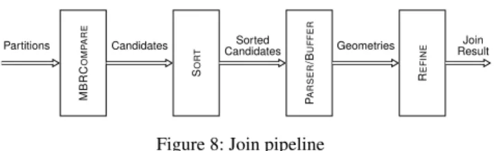
When a spatial join is part of a query, AT-GIS constructs a second pipeline that consumes partitions and emits the joined geometries. This pipeline uses a set of specialised transducers to implemented a PBSM join algorithm [48]. This permits the join to execute along-side other transducers if further selection or aggregation is needed. Since the partitions are non-disjoint, there is a possibility of dupli-cate results in the output, which are removed by a sequential step prior to returning the query result.
The PBSM join is realised as ajoin pipelineof ATs, operating on the spatial partitions (see Fig. 8). The partition has two lists of
Name Description Size (GB) Shapes (1000s)
OSM-X OpenStreetMap XML 592 187,560
OSM-G OpenStreetMap GeoJSON 63.3 187,560
OSM-W OpenStreetMap WKT 41.0 187,560
OSM-10G OpenStreetMap replicated 633 1,875,600
Synthn,σ Synthetic dataset 10.0 n/1000
Table 2: Spatial datasets used for evaluation
MBRs and the offset in the original data of the corresponding object. Storing the offsets means that objects can be re-parsed on demand, avoiding the need to keep the entire dataset in memory.
The join pipeline first finds all MBR intersections in a parti-tion (MBR COMPAREtransducer) and passes a stream of poten-tially matching candidates to the SORTtransducer. SORTbuffers the stream until a threshold is reached, and then sorts the objects by location in the input data. The aim is to position candidates involv-ing the same objects adjacently so that the time that objects remain in memory is bounded. As adjacency can only be achieved for one of the two sets of objects being joined, AT-GIS makes the largest set adjacent. The PARSER/BUFFER transducer re-parses objects to construct the full geometry for refinement. A hash map stores objects in the non-adjacent stream to limit repeated parsing. Once a block is processed, the hash map is cleared. Finally, the REFINE transducer performs the join test, such as geometry intersection.
Storing entire objects in memory can potentially exhaust avail-able resources. By adjusting the threshold in SORT, the number of stored objects can be reduced. While reducing memory usage, some objects may have to be read several times when the entire partition cannot be processed as a single sorted block.
As objects can appear in multiple spatial partitions, duplicate matches may be part of the final result. To mitigate this, after the join pipeline has finished, AT-GIS sorts the result by the offsets of both objects joined and eliminates duplicates.
If additional processing is required on the joined objects, this can either be added to the end of the join pipeline or as a separate phase after duplicate elimination. As objects are only retained in memory while needed by the pipeline, running algorithms as a separate stage may require objects to be re-parsed. Executing computation inside the pipeline provides immediate access to the joined objects at the expense of potentially encountering duplicate results, which need to be removed.
5.
EVALUATION
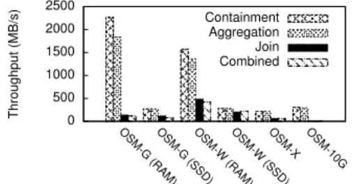
We evaluate AT-GIS experimentally: we compare its performance against other approaches (§5.1) and use synthetic and real-world datasets to explore scalability (§5.2), different data formats (§5.3), different filtering pipelines (§5.4), dataset skew (§5.5) and parti-tioning options (§5.6).
Datasets.Table 2 summarises our datasets. We use the OpenStreet-Map dataset [44], retrieved on May 18, 2015. This is a large real-world dataset that is widely used to benchmark spatial query pro-cessing. In addition to the orignal XML file (OSM-X), we prepare two additional versions: a GeoJSON-formatted one (OSM-G) and a WKT-formatted one (OSM-W), which is used for loading into PostGIS, MonetDB and SpatialHadoop. We also create a version in a proprietary format of a commercial DBMS. In addition to the geometry, we add an objectidinto each object as metadata.
To evaluate scalability as the data sizes grow beyond the available memory, we create a larger dataset (OSM-10G) by replicating the OpenStreetMap dataset 10 times. For each replication, the geome-tries are kept the same but theidis changed to ensure uniqueness.
We also generate a synthetic dataset (Synth) that includes poly-gons and multi-polypoly-gons with the number of edges distributed ac-cording to a log-normal distribution. Two parameters control the
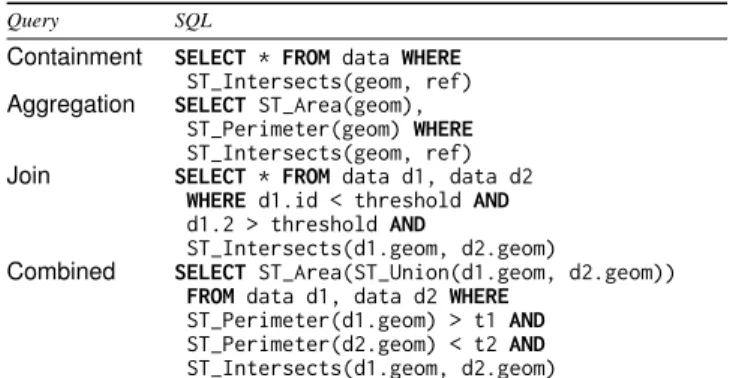
Query SQL
Containment SELECT * FROM data WHERE
ST_Intersects(geom, ref)
Aggregation SELECT ST_Area(geom), ST_Perimeter(geom) WHERE
ST_Intersects(geom, ref)
Join SELECT * FROM data d1, data d2
WHERE d1.id < threshold AND
d1.2 > threshold AND
ST_Intersects(d1.geom, d2.geom)
Combined SELECT ST_Area(ST_Union(d1.geom, d2.geom))
FROM data d1, data d2 WHERE
ST_Perimeter(d1.geom) > t1 AND
ST_Perimeter(d2.geom) < t2 AND
ST_Intersects(d1.geom, d2.geom) Table 3: Spatial SQL queries used for evaluation number of geometries and theσvalue of the distribution. The size of the geometries is scaled so that the dataset is 10 GB.
Queries.We use four types of spatial SQL queries, as shown in Table 3: acontainmentquery that selects all polygons contained within some bounding box; anaggregationquery that combines containment with a summary function over all of the matching polygons—in our case, we use the total perimeter and total area; ajoin query for which we split the input data into two disjoint subsets and which finds all intersecting pairs; and, finally, we use
a combinedquery to show how AT-GIS handles more complex
pipelines consisting of two containment queries to determine the input to a join, followed by an aggregation on the resulting pairs. Experiments with queries that use other geometries and predicates give similar results.
As our input data is geographic, we perform all of our compu-tation using a spherical coordinate system. We use two methods to calculate the linear distance between points when performing perimeter calculations: by default, we use spherical projection, but, in §5.4, we also employ the more accurate but more expensive computation using Andoyer’s algorithm [4].
AT-GIS implementation.Our prototype is implemented in C++. All geometric operations use theBoost::Geometry[17] library, other than the MBR intersection testing, which is hand-written. Aside from the partially-associative JSON parsing, which is done
byRapidJSON[50], all other transducers are implemented by us.
The created AT pipelines for a given query plan are compiled by the GNU g++ compiler. Compilation takes up to 5 seconds, which is negligible compared to the total runtime.
AT-GIS is executed using both fully- and partially-associative transducers to determine the level of optimisation available from reducing speculation: AT-GIS-FATruns all queries using a fully-associative pipeline with no optimisation;AT-GIS-PATuses opti-mised parsers when speculation can be reduced.
System comparisons.We takeHadoop-GIS[1] as an example of a distributed cluster system, which does not use stored indexes beyond the initial partitioning, andSpatialHadoop[13] as an index-based solution. We also compare toPostGIS[25],MonetDB[59] and a commercial DBMS with spatial support (DBMS-X) in terms of single-node spatial query engines. The performance results for
SpatialHadoop,PostGIS,MonetDBandDBMS-Xresults are mea-sured on the same machine as AT-GIS; the results for Hadoop-GIS are based on the same dataset and taken from the paper [1].
ForMonetDB, the default set-up has one table with one row per object; inPostGIS, the table is manually sharded into 1000 ranged partitions; andDBMS-Xuses a 1024-way spatially partitioned table. The table is indexed by the geometry and clustered by the index prior to query execution.
The experiments are performed using both bounding-box ( Post-GIS-B, MonetDB-B) and full-geometry comparisons (PostGIS-G,
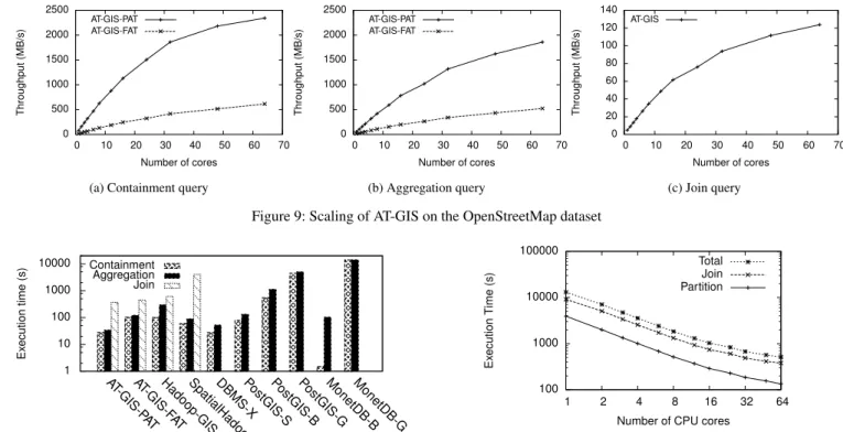
0 500 1000 1500 2000 2500 0 10 20 30 40 50 60 70 Throughput (MB/s) Number of cores AT-GIS-PAT AT-GIS-FAT
(a) Containment query
0 500 1000 1500 2000 2500 0 10 20 30 40 50 60 70 Throughput (MB/s) Number of cores AT-GIS-PAT AT-GIS-FAT (b) Aggregation query 0 20 40 60 80 100 120 140 0 10 20 30 40 50 60 70 Throughput (MB/s) Number of cores AT-GIS (c) Join query Figure 9: Scaling of AT-GIS on the OpenStreetMap dataset
1 10 100 1000 10000 AT-GIS-P AT AT-GIS-F AT
Hadoop-GISSpatialHadoopDBMS-XPostGIS-SPostGIS-BPostGIS-GMonetDB-BMonetDB-G
Ex ecution time (s) Containment Aggregation Join
Figure 10: Comparison of query execution times
MonetDB-G). We also manually sharded the PostGIS installation (PostGIS-S). All experiments are repeated and have low variance, which is why we omit error bars.
Experimental set-up.All experiments are performed on a quad-socket, 64-core AMD server with 128 GB RAM. Each CPU has a nominal clock speed of 2.3 GHz, with turbo mode increasing this to 2.9 GHz for small numbers of threads. To limit the effects of I/O bottlenecks, experiments using theOSM-G,OSM-WandSynth
datasets read the data from a RAM disk. For experiments using the
OSM-10GandOSM-Xdatasets, we load the data onto an SSD and ensure that the OS file cache is cleared. A second SSD is used to store any temporary data files.
5.1
Query performance
Fig. 10 shows the execution time for three of our queries on different systems.1Executing from RAM,AT-GIS-PATachieves the same query execution time asDBMS-Xfor the containment query and takes 30% less time for aggregation queries, despite not pre-loading and indexing the data. The results also show the benefit ofAT-GIS’s efficient pipelining: aggregation takes only 25% longer than containment, outperforming the other comparable systems.
Of all of the RDBMS,MonetDBhas the fastest query time for MBR-only queries: using a combination of sequential data access and multithreading, it outperforms the index-basedPostGIS and
DBMS-Xas well asAT-GIS. Once full geometry comparisons are considered, however, the lack of spatial optimisations inMonetDB
results in it performing the slowest of all systems.
The results also show that current RDBMS are not optimised for large spatial joins, even with hand-optimised query plans: both
PostGISandDBMS-Xdo not complete the join within 24 hours, and
MonetDBconstructs the cross-product of the input prior to joining, 1We do not use the combined query for comparison because the other systems exhibit excessive time or memory requirements when performing the join first.
100 1000 10000 100000 1 2 4 8 16 32 64 Ex ecution Time (s)
Number of CPU cores Partition
Join Total
Figure 11: Partition and join query scaling to 64 CPU cores requiring over 17 TBs of memory. While executing on a single node,AT-GIS-PATis 10× faster thanSpatialHadoop for the join query due to the latter’s cluster management and communication overhead.Hadoop-GISexhibits the closest join performance to AT-GIS, however, it is deployed on a cluster with more than 3×the number of CPU cores of our server.
For the containment and aggregation queries, the communica-tion overhead of the distributed frameworks becomes even more apparent.Hadoop-GISrequires 3×longer for the aggregation query than for the containment query—the largest disparity of all systems. Taking the number of CPU cores into account,Hadoop-GISrequires 30×the computation resources ofAT-GIS-PAT. The upfront indexing ofSpatialHadoopimproves performance compared toHadoop-GIS, but it still trails behindAT-GISon a single node.
The difference betweenAT-GIS-PATandAT-GIS-FATfor the con-tainment and aggregation queries shows the dominance of the data parsing cost in terms of the total execution time. Note that the execution times for the other systems do not take the time to load the data into account because this may be amortised over multiple queries. Loading the data can take significant time though, ranging from 30 minutes forMonetDBto over 4 hours forDBMS-X. The data format may also need to be converted prior to loading—no system other thanAT-GIScan handle raw OSM XML data.
5.2
Scalability
Next we consider howAT-GISscales as we vary the number of CPU cores. Figs. 9a and 9b show both full and partial ATs scale to 32 CPU cores for containment and aggregation queries. There are two changes of the gradients in the scaling results: the first occurs after 16 CPU cores and is due to the overclocking of cores with few threads on the AMD CPU; the second change at 32 CPU cores is due to its micro-architecture: the CPU only has 32 FPU units shared between 64 cores. As AT-GIS executes floating-point intensive operations, the scaling beyond 32 cores becomes limited. The contention for FPUs is less of an issue forAT-GIS-FATbecause it includes more integer operations when parsing the data.