yin-han chung
M O D E L L I N G T H E X B O X 3 6 0 K I N E C T F O R V I S U A L S E RV O C O N T R O L A P P L I C AT I O N S
M O D E L L I N G T H E X B O X 3 6 0 K I N E C T F O R V I S U A L S E RV O C O N T R O L A P P L I C AT I O N S
yin-han chung
A research report submitted to the Faculty of Engineering and the Built Environment, University of the Witwatersrand, Johannesburg, in partial fulfilment of the requirements for the degree of Master of Science in Engineering.
Yin-Han Chung:Modelling The Xbox360Kinect for Visual Servo Control Applications,M.Sc. Research Report, August2016
supervisors: Jacques Arno Naudé Michaël Antonie van Wyk department:
School of Electrical and Information Engineering faculty:
Engineering and the Built Environment institution:
D E C L A R AT I O N
I declare that this research report is my own unaided work, other than where specifically acknowledged. It is being submitted for the degree of Master of Science in Engineering to the University of the Witwatersrand, Johannesburg. It has not been submitted before for any degree or examination to any other university.
. . . day of . . . year . . . .
A B S T R A C T
There has been much interest in using the Microsoft Xbox360Kinect cameras for visual servo control applications. It is a relatively cheap device with expected shortcomings. This work contributes to the prac-tical considerations of using the Kinect for visual servo control appli-cations. A comprehensive characterisation of the Kinect is synthesised from existing literature and results from a nonlinear calibration proce-dure. The Kinect reduces computational overhead on image process-ing stages, such as pose estimation or depth estimation. It is limited by its 0.8 m to 3.5 m practical depth range and quadratic depth res-olution of 1.8 mm to 35 mm, respectively. Since the Kinect uses an infra-red (IR) projector, a class one laser, it should not be used out-doors, due to IRsaturation, and objects belonging to classes of non-IR-friendly surfaces should be avoided, due to IR refraction,
absorp-tion, or specular reflection. Problems of task stability due to invalid depth measurements in Kinect depth maps and practical depth range limitations can be reduced by using depth map preprocessing and activating classical visual servoing techniques when Kinect-based ap-proaches are near task failure.
To my parents, for their love and support.
A C K N O W L E D G M E N T S
I wish to thank my supervisors, Jacques Naudé and Antonie van Wyk, for their invaluable support and guidance.
My research has been, many a time, set on a one-way flight back to nowhere, which was averted with Jacques’ paranoid optimism. You have my most sincere gratitude.
Additionally, I wish to acknowledge:
• Mark Goosens of the Wits Genmin Laboratory, for machining the wooden calibration board.
• All the folks who spent time in the coffee room, for their thought-ful conversations.
• André Miede, for the ClassicThesis LaTeX template on which this document is based.1
• The National Research Foundation (NRF) of South Africa, for the funding of this research.2
1 http://www.miede.de
2 http://www.nrf.ac.za/
C O N T E N T S
Abstract v List of Figures x List of Tables xii List of Symbols xiii
Acronyms xv
1 introduction 1
1.1 Research Questions 2
1.2 Methodology 2
1.3 Structure of the Research Report 2
2 literature review 3
2.1 Visual Servoing 3
2.1.1 Basic Techniques 5
2.1.2 Stability, Robustness, and Sensitivity 6
2.1.3 Advanced Techniques 8
2.2 Microsoft Kinect 10
2.2.1 Kinect-based Research 10
2.2.2 Software Drivers 11
2.2.3 Depth Sensor Design 12
2.2.4 Kinect Disparity Models 12
2.2.5 Depth Resolution and Accuracy 13
2.2.6 Calibration 13
2.2.7 Depth Distortion 14
2.2.8 Depth Sensor Interference and Noise 14
2.3 Summary 15
3 geometric camera modelling 16
3.1 Planar Transformations 16
3.1.1 Translation 16
3.1.2 Rotation 17
3.1.3 Relative Pose 17
3.2 Image Formation 19
3.2.1 Thin Lens Optics and Focus 21
3.2.2 Perspective Transform 24
3.2.3 Normalised Image Plane 25
3.2.4 Geometric Lens Distortion 26
3.3 Pixels, Image Sensors and Digital Images 27
contents ix 3.3.1 Field of View 29
3.3.2 Sensor Spatial Resolution 29
3.4 Intrinsic Parameters 30
3.5 Extrinsic Parameters 30
3.6 Summary 31
4 kinect camera characterisation 32
4.1 Components 32
4.2 Specifications 33
4.3 Depth Camera Characterisation 34
4.3.1 IR Speckle Pattern 34
4.3.2 Disparity 35
4.3.3 Spatial Disparity Distortion 36
4.3.4 Depth Resolution 37
4.4 Calibration Experiment 38
4.4.1 Image Capturing Tool 38
4.4.2 Calibration Rig 38
4.4.3 Procedure 39
4.5 Calibration Results 41
4.5.1 RGB Reprojection Error 43
4.5.2 RGB Lens Distortion 44
4.5.3 Depth Reprojection Error 45
4.5.4 Spatial Disparity Distortion 47
4.5.5 Disparity and Depth Resolution 47
4.5.6 Extrinsic Parameters 48
4.5.7 Post-calibration Specifications 49
4.6 Summary 50
5 visual servoing implications 51
5.1 Basic Visual Servoing Techniques 51
5.1.1 Task Function 51
5.1.2 Image-Based Visual Servoing 52
5.1.3 Position-Based Visual Servoing 56
5.2 Kinect Integration 57 5.2.1 Depth Measurements 58 5.2.2 Depth Resolution 58 5.2.3 IR Light Limitations 59 5.2.4 Depth Holes 59 5.2.5 Out-of-Bounds 59 5.2.6 Sensor Bandwidth 60 5.3 Summary 61 6 conclusion 62
7 recommendations for future research 63
L I S T O F F I G U R E S
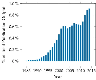
Figure2.1 Ratio ofvisual servoingpublications to total
pub-lication output, based on the IEEE Xplore database. 3
Figure2.2 The Kinect for Xbox360. 10
Figure3.1 Two-dimensional translation. 16
Figure3.2 Two-dimensional rotation. 17
Figure3.3 Relative pose between two coordinate frames. 18
Figure3.4 Objects in three-dimensional space. 18
Figure3.5 Coordinate frames in three-dimensional space. 19
Figure3.6 Ray tracing from a point source to a pinhole camera. 19
Figure3.7 Ideal pinhole image formation. 20
Figure3.8 Blurred pinhole image formation. 20
Figure3.9 A lens converges collimated light to its focal point. 21
Figure3.10 Optical centre, focal plane, and image plane. 21
Figure3.11 Thin lens optics. 22
Figure3.12 Pan and tilt. 22
Figure3.13 Viewing objects from an angle. 22
Figure3.14 Thin lens behaviour using focal length multi-ples. 23
Figure3.15 Focused image formation using a lens. 24
Figure3.16 three-dimensional point projection through an equivalent pinhole. 24
Figure3.17 Central projection model. 25
Figure3.18 Normalised image plane and coordinates. 25
Figure3.19 Radial and tangential lens distortions on the normalised plane. 26
Figure3.20 Pixel coordinate frame on the front image plane. 28
Figure3.21 Square rendering of pixels. 28
Figure3.22 Vertical field of view. 29
Figure3.23 World coordinate frame. 31
Figure4.1 Kinect point of view. 32
Figure4.2 Kinect cameras and projector. 33
Figure4.3 Kinect product information. 33
Figure4.4 Kinect IR images. 35
Figure4.5 Depth resolution. 37
Figure4.6 Full calibration setup. 39
Figure4.7 Calibration target plane rotations. 39
Figure4.8 Corner extraction and plane selection of cali-bration rig. 40
List of Figures xi Figure4.9 Kinect-centred, top-down view of plane
rota-tion data sets. 42
Figure4.10 Plots and histograms of RGB corner reprojec-tion errors. 43
Figure4.11 RGB-full lens distortions. 44
Figure4.12 Undistorting an image using the distortion model. 45
Figure4.13 Plots and histograms of depth reprojection er-rors. 46
Figure4.14 Absolute valued spatial disparity distortion im-agesDδ(u,v). 47
Figure4.15 RGB-full disparity, depth and depth resolution. 48
Figure4.16 RGB-full image registration using extrinsic pa-rameters. 49
Figure4.17 RGB-standard image registration using extrin-sic parameters. 49
Figure4.18 Comparing RGB-full and -standard colour im-age sizes. The yellow strip indicates pixels cropped by the Kinect. 50
Figure5.1 Image-based visual servoing 54
Figure5.2 Position-based visual servoing 55
L I S T O F TA B L E S
Table 4.1 Kinect documented specifications. 34
Table 4.2 Kinect image data sizes and data rates. 34
Table 4.3 Kinect depth resolution. 37
Table 4.4 RGB camera calibration results. 41
Table 4.5 Depth camera calibration results. 41
Table 4.6 RGB reprojection error comparison between data sets. 43
Table 4.7 RGB lens distortion coefficient comparison be-tween data sets. 45
Table 4.8 Depth reprojection error comparison between data sets. 45
Table 4.9 Disparity coefficient comparison between data sets and authors. 47
Table 4.10 Disparity model singularity for RGB-full and -standard. 48
Table 4.11 Kinect post-calibration RGB specifications. 49
Table 4.12 Kinect post-calibration depth specifications. 50
L I S T O F S Y M B O L S
α0,α1 depth distortionαcoefficients
a camera characteristics c0,c1 Kinect disparity coefficients {C} coordinate frame
δr additive radial lens distortion ∆r multiplicative radial lens distortion δs small error due to finite bandwidth δt tangential lens distortion
Dδ(u,v) depth distortionβcoefficients d Kinect disparity [kdu]
dk undistorted Kinect disparity [kdu]
e(t) task function error
f focal length [mm]
f focal point
H image sensor vertical pixel count [px]
I identity matrix
k1,k2,k3 radial lens distortion coefficients
K camera matrix
Kp projection matrix λ controller gain
L image Jacobian, or interaction matrix
L+ pseudo-inverse of the interaction matrix
m(t) set of image measurements
ν camera linear velocity ω camera angular velocity
Ωa available bandwidth
Ωc corner frequency of the desired sensitivity function p pole of a transfer function
p1,p2 tangential lens distortion coefficients
p two-dimensional image point ¯
p augmented image point
pn normalised image point
list of symbols xiv
pdn distorted normalised image point
P three-dimensional world point ¯
P augmented world point
Ph vertical camera spatial resolution [m/px/m] Pw horizontal camera spatial resolution [m/px/m] ρh vertical pixel pitch [m/px]
ρw horizontal pixel pitch [m/px]
R rotation matrix
s set of visual features S(jω) sensitivity function
Smin smallest sensitivity penalty
θu Euler axis/angle θh horizontal field of view θv vertical field of view θ angle of rotation t scalar translation
[t]× cross product matrix of a vectort
T homogeneous transformation, or pose, matrix A
BT relative pose of frame {B} with respect to {A}
X translation matrix
υ camera spatial velocity
u0 horizontal principle point [px] v0 vertical principle point [px]
W image sensor horizontal pixel count [px] ξ relative pose
z(d) Kinect depth [m]
zk(d) undistorted Kinect depth [m]
zw distance between world point and lens [mm] zi distance between lens and image point [mm]
A C R O N Y M S
DOF Degree of Freedom EKF Extended Kalman Filter fps frames per second
GPU Graphics Processing Unit IBVS Image-Based Visual Servoing ICP Iterative Closest Point
IR infra-red
KCT Kinect Calibration Toolbox kdu Kinect disparity units NUI Natural User Interface
OpenCV Open Source Computer Vision PBVS Position-Based Visual Servoing PCL Point Cloud Library
PGM Portable Grey Map PPM Portable Pix Map px pixel
RGB Red Green Blue, primary colour model ROS Robot Operating System
SDK Software Developer Kit SURF Speeded Up Robust Features URL Uniform Resource Locator USB Universal Serial Bus
1
I N T R O D U C T I O N
Robotics is the intelligent connection of perception to action. — Michael Brady [1]
The problem of guiding a robot’s actions using visual feedback from a camera arose at least four decades ago [2]. The modern term for this is visual servoing. Visual servoing requires, at minimum, a single camera, but, with the availability of RGB-D cameras, classical visual servoing techniques have been reinvestigated and new methods and applications have been developed.
The first industrial robots were envisioned to make manufacturing more economical than cam control systems, by being adaptable to new tasks [3]. As tasks grew in complexity, so did the fixtures that were required to fix objects to precise locations for the robot to inter-act with, negating the robot’s general-purpose or flexibility [4]. A robot without sensory feedback of its environment requires its en-vironment to be structured. The enen-vironment must be co-engineered to facilitate the specific robot [5] and the robot must know, a priori, the location of objects it interacts with. Visual feedback can reduce the required tolerance on the expected location of objects [6], allow-ing the robot to work in a more unstructured environment without explicit reprogramming of existing tasks.
There has been much interest in using the Microsoft Xbox360Kinect camera for visual servoing applications [7–14]. Of these applications, some do not explicitly state if they consider camera calibration and depth distortion modelling [7, 8, 10, 13, 14], and some do not con-sider the Kinect’s limitations, such as the depth camera’s sensitivity to sunlight [9] or its near range limitation [13,14].
Since the Kinect is a relatively cheap device, it is expected to have its shortcomings. This research models the Kinect’s RGB and depth cam-eras, conducts joint camera calibration using the Kinect Calibration Toolbox (KCT) by Herrera [15], characterises the devices limitations,
and investigates some of the consequences of using the Kinect cam-era for visual servo control applications.
1.1 research questions 2 1.1 Research Questions
This research addresses the questions:
1. How are the Kinect RGB and depth cameras modelled?
2. What practical considerations does the Kinect impose on visual servo control applications?
1.2 Methodology
The research questions are addressed by following these steps: • Model the Kinect RGB camera using the pinhole camera model. • Model the Kinect depth camera using supporting literature. • Calibrate the Kinect cameras using theKCTby Herrera [15].
• Characterise the limitations of the Kinect device.
• Given the calibrated models and limitations, discuss some of the consequences of using the Kinect for visual servo control applications.
1.3 Structure of the Research Report
Chapter2covers relevant literature on visual servoing, its limitations, and Kinect camera modelling and calibration.
Chapter 3covers briefly the topics of: pose, image formation, image distortion, image sensors, and the intrinsic and extrinsic camera pa-rameters. Readers familiar with these topics can skip this chapter. Chapter4 shows the Kinect characterisation, discusses and conducts the calibration procedure, and analyses the results.
Chapter5covers basic visual servoing techniques, and discusses some of the consequences of using the Kinect for visual servo control appli-cations.
Chapter 6 addresses the research questions and concludes this re-search.
2
L I T E R AT U R E R E V I E W
A literature survey on the basic techniques, advanced techniques, and problems of visual servoing is presented. Additionally, visual servo-ing in the context of the Kinect is presented. Kinect topics are then discussed separately, in particular, its sensor design, characterisation, calibration, depth distortion models, interference, and noise.
2.1 Visual Servoing
The earliest found IEEE visual servoing publication was released in 1985(Figure2.1), butvisual feedbacktechniques date past four decades.
Shirai and Inoue’s 1973publication [16] is generally regarded as the first to show end-effector positioning using visual feedback.
1985 1990 1995 2000 2005 2010 2015 0% 0.2% 0.4% 0.6% 0.8% 1.0% Year % of Total Publication Output
Figure2.1: Ratio of visual servoingpublications to total publication output, based on the IEEE Xplore database.
To the author’s knowledge, Agin [17] first used the termvisual servo-ingin1977at SRI International, for coarse positioning of an industrial manipulator mounted with a camera for a bolt insertion task.
Most of the basic visual servoing fundamentals were established by the early1990s, which followed with the first visual servoing tutorial by Hutchinson et al. [18] in 1996.
2.1 visual servoing 4 Early advanced techniques were developed at the turn of the mil-lennium, which followed with updated tutorials by Chaumette and Hutchinson [19,20] in 2006and2007respectively.
Visual servoing schemes can be classified in a number of ways. The main classifications are based on: use of dynamic, closed-loop visual feedback control; use of the robot’s closed-loop joint control; use of a three-dimensional target object model; and camera configuration. Early visual feedback systems, static look-and-move, cycled a closed-loop joint controlled robot through a sequence of three mutually ex-clusive steps to complete a task [21]: look, plan, and move. While the robot was busy moving, it could not look or plan the next incremental position to move. While these systems had elements of visual sensing, they lacked dynamic control, hence they are no longer used.
Later visual servo systems,dynamic look-and-move, executed every step in parallel [21]. These systems used a closed-loop visual feedback controller to output velocity commands to the joint controller, making the system more responsive, but dynamic performance and stability must be evaluated for acceptable transient response.
Anindirectsystem is synonymous with a dynamic look-and-move sys-tem [22]. In contrast, a direct system uses the vision-based controller to directly stabilise a robot with no joint controller [21].
Weiss et al. [21] originally proposed the distinction between visual servo (direct) systems and dynamic look-and-move systems. The term, dynamic look-and-move, is depreciated, and now visual servo sys-tems generally refer to indirect syssys-tems [4]. Indirect systems are pre-ferred because a joint controller handles low sampling rates from the camera and robot dynamics and kinematic singularities are hidden from the vision-based controller [18]
In model-based visual servoing, the three-dimensional model of the target object is available [22]. The target object model and camera intrinsic parameters are required for pose (position and orientation) estimation algorithms. Otherwise, the method is model-free.
Aneye-in-hand, orend-point closed-loop, system mounts the camera by the robot’s end-effector. Camera motion is coupled to the robot’s mo-tion. An eye-to-hand, or end-point open-loop, system has the camera fixed in the workspace observing the target object and robot [4].1 For visual servoing task functions, the desired end-effector reference is specified using either predefined Cartesian references or taught image references [23].
2.1 visual servoing 5 Predefined Cartesian references are naturally specified using pose, usually from a known model, but cause the steady state end-effector pose accuracy, or sensitivity, to suffer in the presence of camera cal-ibration errors, robot calcal-ibration errors, and target object modelling errors [24].
Taught image references are obtained via an offline method, teach-by-showing [25], where the robot’s end-effector is brought to the desired end-effector pose and a corresponding image is captured, or taught. Calibration and modelling errors are partially circumvented [24]. 2.1.1 Basic Techniques
There are two basic approaches to visual servoing: Position-Based Vi-sual Servoing (PBVS), or three-dimensional visual servoing; and
Image-Based Visual Servoing (IBVS), or two-dimensional visual servoing.2
These control schemes are identified by their feedback signal. The strengths and weaknesses of each method is discussed.
PBVS control schemes regulate end-effector pose in Cartesian space.
Pose estimation is used to determine the relative pose error from the desired end-effector pose. This method bears resemblance to regulat-ing a robot along a geodesic Cartesian trajectory.
There are few publications onPBVS. Westmore and Wilson [26] investi-gated the feasibility and performance of using the Extended Kalman Filter (EKF) for real-timePBVS. Their static object experiment was
suc-cessful, but it was limited to two-dimensional position control. The three-dimensional control case and complete PBVS design
methodol-ogy was later demonstrated by Wilson et al. [27].
SincePBVSregulates pose, and not the image, the resulting Cartesian
trajectory does not guarantee that the image features of a target object stays within the camera’s field of view (a visibility constraint), which causes pose estimation to fail. Such a problem can be avoided by using trajectory planning [4] or certainPBVScontrol laws [23].
IBVScontrol schemes regulate image features directly in image space. The position of a set of image features implicitly defines a pose. By extension, the current image and reference image implicitly define the current pose and reference pose, respectively. Hence, regulating the current image to look like the reference image should move the end-effector towards the desired pose.
Sanderson and Weiss [28] proposed the first directIBVSsystem.
Simu-lations of direct IBVSusing adaptive control techniques were demon-strated by Weiss et al. [25], but were limited to three or less Degree of 2 Position-based and pose-based visual servoing are used interchangeably.
2.1 visual servoing 6 Freedom (DOF) manipulators due to the low sampling rate and time delay of their image processing system. An indirect4-DOF IBVSsystem
was later shown by Feddema and Mitchell [29], who overcame the vision sampling rate problems using an asynchronous feature-based trajectory generator. An indirect6-DOF IBVSsystem was demonstrated
by Rives et al. [30] and Chaumette et al. [31], who formalised visual servoing analysis using the task function approach.
In contrast toPBVSlosing sight of the target object,IBVScontrol schemes have no control over their Cartesian trajectories. Given the position of an image point in the current image and its position in a reference image, theIBVScontrol law pushes this image point from its current position in a straight line towards its reference position. This trajec-tory, or the image feature trajectrajec-tory, requires the robot’s joints to do unnatural movements. If large rotations about the camera’s optical axis are required, the robot may exceed its joint limits [23].
IBVS requires computation of the image Jacobian, or interaction
ma-trix, which relates camera spatial velocity to image feature velocity. The image Jacobian’s form depends on the choice of image features, with point features being the most common form. Rives et al. [30] solved the image Jacobian for geometric primitives, such as points, lines, and circles. Other image features include ellipses [32] and im-age moments [33,34].3
Most image Jacobians are a function of feature depth. Depth can be measured or estimated. Online estimation solutions to this problem include: partial three-dimensional reconstruction [29], constant depth [32], adaptive control [35], and depth from image and robot motion [36]. A depth-independent image Jacobian approach is presented here [37], but only for eye-to-hand (fixed camera) systems.
2.1.2 Stability, Robustness, and Sensitivity
IBVS with taught image references is known to be tolerant towards
image quantisation errors, measurement noise [38] and camera cali-bration errors [39] - that is, systematic errors. Hence the errors from the reference and measurement cancel out. Despite this, a case ofIBVS
failure due to poor camera calibration and noise has been reported in [40], and, even with accurate camera calibration, care must be taken with regards to depth estimation errors of the target object [41,42]. In contrast, PBVS control is generally said to be unstable in the
pres-ence of sensor errors. This is an often citedPBVSdisadvantage.
Janabi-sharifi et al. [23] argued thatPBVSinstability is due to the use of prede-fined Cartesian references. They said thatPBVSandIBVSperformance
2.1 visual servoing 7 is expected to be the same when both schemes use the same refer-ence type (predefined or taught referrefer-ences), and performance should be evaluated with a common framework.
Given a common framework, the performance issues lie with the cam-era, target object, and robot modelling errors. Under these errors [23]: image feature trajectories will warp when using taught image refer-ences; and the steady state error will increase when using predefined Cartesian references.4
Local asymptotic stability of IBVS was shown by Espiau et al. [32], making IBVS a local-only control method; if the initial camera
dis-placement (relative to the target pose) is too large, the current pose may fail to converge to the desired pose.
At least three point features are required for IBVS control schemes,
such that the image Jacobian matrix has a rank of six and the image Jacobian inverse exists. Then, the camera motion equations can be solved, but this solution is not unique. There are four solutions [43], or global minima, where both the camera spatial velocity and control error, or task function error, are zero. A unique solution is available if at least four point features are used, for which the image Jacobian pseudo-inverse has a least squares error solution [38].
When using four or more image point features, the dimension of the image Jacobian pseudo-inverse kernel is non-zero. This indicates that sometimes local minima exist [43], that is, camera spatial velocity is zero and the task function error is non-zero. If aIBVScontrol law with
a constant image Jacobian pseudo-inverse is used, the unique global minimum can be reached. Nonetheless, this control law sometimes causes image point features to leave the camera’s field of view, caus-ing the image Jacobian to become rank deficient.
Tasks requiring a rotation around the (optical) z-axis follow unsatis-factory Cartesian trajectories, asIBVSenforces shortest image feature
trajectory. Instead of rotating, a backwards camera translation hap-pens first before moving towards the target object. This effect is called camera retreat, which is a result of motion control coupling [43]. A required180° rotation about the z-axis is an extreme case which re-sults in task singularity. The initial and desired image point features are reflections about the camera’s principal point. Camera retreat oc-curs towards depth at infinity, where all image point features lie at the centre of the image, or principal point. Either the robot becomes joint-limited first, or the image Jacobian becomes rank deficient. Also on 180° rotation problems, some IBVS control laws cause a for-wards camera translation (camera advance) tofor-wards depth at zero, 4 Trajectory warping increases the task convergence time, since regulating along a
2.1 visual servoing 8 where hopefully all image point features are out of the camera’s field of view before colliding with the target object.
These characteristic problems of IBVS, local minima and motion
con-trol coupling, do not exist for PBVS [23].5 PBVS problems usually
in-volve pose estimation algorithms and visibility constraints, which incur computational costs. Characteristic problems of IBVS are
ad-dressed by advanced visual servoing techniques. 2.1.3 Advanced Techniques
Several categories of (early) advanced visual servo schemes exist that mix PBVS and IBVS behaviour together to avoid their respective
dis-advantages. Major categories are covered, but only a handful of com-monly encountered schemes are discussed.
Hybrid techniques, such as the Koichiro Deguchi (or KD) method [45] and2-1/2-D visual servo [46], have been proposed. These techniques are homography-based, which find the plane-to-plane relationship, or homography matrix, between the current and reference images. The homography matrix is then decomposed into separate rotation and translation quantities for decoupled motion. Since motion control is decoupled, IBVS local minima can be avoided. Additionally, partial
camera displacement estimation using the homography matrix does not require the three-dimensional object model.
With homography-based approaches, however, at least four and eight matching image feature points are required for coplanar objects and non-coplanar objects, respectively. The homography matrix is also susceptible to noise, which makes the performance of hybrid schemes degrade more than plainIBVSapproaches [47].
Specifically, the KD method [45] is designed around the visibility con-straint and translation motion is constrained to take the shortest path, but it does not address task singularity and stability issues. In con-trast,2-1/2-D visual servo [46] designs for robustness [48] and a task singularity free workspace, but adaptive control of gain and system parameters is required to enforce the visibility constraint, which in-flicts a slow time-to-convergence due to gain adaptation.
For partitioned visual servo schemes, the XY/Z partitioned scheme by Corke and Hutchinson [44] acknowledged that motion control cou-pling is a z-axis translation phenomenon and task singularities are a z-axis rotation phenomenon. These two motion controls are isolated, which involves computing two computationally inexpensive image
2.1 visual servoing 9 features that are mutually motion decoupled. Still, this method is sus-ceptible to image feature points leaving the camera’s field of view. A simple PBVS andIBVS switching controller was proposed by Gans
and Hutchinson [49]. Each controller had an accompanying Lyapunov function with a chosen threshold. While the PBVS controller was ac-tive, the switch to IBVS control happened when the IBVS Lyapunov
function exceeded its threshold and vice versa. PBVS flaws are
miti-gated, but characteristic problems ofIBVSstill exist.
More recently, authors have taken a different approach, using direct visual servoing methods. In contrast to geometric feature-based vi-sual servoing methods, direct methods do not require any image fea-ture extraction, matching, and tracking, and instead perform align-ment of whole images.6Since whole images are used, there is high re-dundancy, making final positioning errors much smaller than feature-based methods and tasks more robust towards partial occlusions. This is very useful for tasks in complex scenes.
One example of direct methods is photometric visual servoing by Collewet and Marchand [51], where whole image luminance is used as a visual feature. Only the corresponding reference image is re-quired to perform a task, but tasks may diverge due to illumination variations. Variation sensitivity depends on the illumination model. The authors proposed that complex illumination models may provide better insensitivity.
Of particular interest is the direct dense depth map-based visual ser-voing by Teulière and Marchand [13], where the control law uses whole depth maps from a Kinect sensor. Depth maps are insensitive to illumination variations, offering improved stability over photomet-ric visual servoing. Nonetheless, this method’s limitations lie with the Kinect, which has limited range and inability to sense outdoors due to infrared light from sunlight, as it is an active infrared sensor. An extension to Teulière and Marchand [13] was presented by Ho-jaij et al. [14]. They designed a two phase controller which first per-formed coarse positioning using a IBVS controller with Speeded Up
Robust Features (SURF), then switched to the direct controller for fine
positioning. The fine positioning controller is activated when crossing a hardcoded depth threshold with respect to the target object.
Direct methods are essentiallyIBVSmethods with redundant features,
hence they suffer similar limitations. Their Cartesian trajectories are non-optimal. In addition, control laws of direct methods are more nonlinear, so this effect is more pronounced. Experiments by [52] us-ing a hybrid method alleviate this problem.
2.2 microsoft kinect 10 With IBVS, tasks will fail with large initial displacements. Similarly, direct methods fail when there is insufficient overlap between cur-rent and reference images or wider occlusions, that is, they have lim-ited domain of convergence. Improvements to domain of convergence have been proposed using hybrid methods [53] and different optimi-sation techniques [50].
2.2 Microsoft Kinect
The Kinect is Microsoft’s vision and voice sensor, used by their Xbox gaming devices. It has a colour (RGB) camera, a depth camera, a multi-array microphone, and a tilt motor at its base which allows it to pitch [54]. Its depth camera is an IRcamera and projector pair.
Mea-surements are accumulated internally and either raw or processed data is transmitted externally via USB.
Microsoft’s Kinect SDK can be used to infer information such as hu-man body location and track body movement. For game designers, this kind of information is useful for designing transparent user in-terfaces with intuitive controls.7
2.2.1 Kinect-based Research
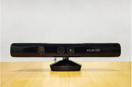
Figure2.2: The Kinect for Xbox360.
The Xbox360Kinect was advertised as a gaming interface (Figure2.2), and, within three months of its November2010release, it sold over10 million units [54]. Its low cost and off-the-shelf availability promoted 7 Otherwise known as a Natural User Interface (NUI).
2.2 microsoft kinect 11 its popularity with researchers. Microsoft termed the development of many creative Kinect applications the “Kinect Effect” [54].
Many open source software organisations developed computer vision library and robotics middleware support, allowing for fast prototyp-ing of Kinect-based experiments.8
Kinect vision-based research and applications have been surveyed ex-tensively by Han et al. [55] and Zhang [54]. In addition, some practical robotics examples include:
• Quadrotor + Kinect by Bouffard et al. [56], a project which re-ceived wide media coverage, and has a YouTube video with over one million views.
• TurtleBot, a personal robot kit from the Open Source Robotics Foundation, Inc. [57] (formerly Willow Garage) for researchers and hobbyists.
• Kinect-based visual servoing: PBVS with redundant joints [7],
object handling [8–10], contour following [11], robust and fast object tracking [12], and direct and hybrid methods [13,14]. • And more recently,Future Robotic Interfacesat NASA’s Jet
Propul-sion Laboratory (JPL) [58], using the improved Kinect2.
2.2.2 Software Drivers
Three drivers are available for communicating with the Kinect [55,59]. Two common choices used for research are the libfreenect driver by OpenKinect and OpenNI driver by PrimeSense.9 The third driver, bundled in the Microsoft Kinect Software Developer Kit (SDK), is
pro-prietary and only runs on Windows7(or above) operating systems. The OpenNI driver is known to enforce factory calibrated settings and give per-pixel depth values in millimetres [60]. Only thelibfreenect driver is able to provide per-pixel disparity values in Kinect dispar-ity units (kdu), which is a widely used metric for comparing depth accuracy measurements [60–63].
8 Organisations such as: Open Source Computer Vision (OpenCV), Point Cloud Library (PCL), and Robot Operating System (ROS)
9 The official PrimeSense sensor module GitHub repository does not contain any com-piled binarieshttps://github.com/PrimeSense/Sensor. Cross-platform binaries can be found in the SensorKinect repository, maintained by a user known as avin2
https://github.com/avin2/SensorKinect. PrimeSense was acquired by Apple Inc. andofficialsupport for OpenNI has since dropped.
2.2 microsoft kinect 12 2.2.3 Depth Sensor Design
Since the Kinect’s hardware is proprietary, its technology is undis-closed. Early efforts to understand the Kinect were published as in-formal online sources.10According to Zhang [54], Microsoft licensed their depth-sensing technology from PrimeSense. Since there is no direct link, Kinect characterisation authors [61,62,65–67] have specu-lated that the technology is explained in the patent by Freedman et al. [68], which was assigned to PrimeSense.
Freedman et al. [68] explains that PrimeSense’s technology computes the three-dimensional coordinates of points using triangulation. Com-puting such a point requires the point to be visible in at least two im-ages, each from a different view [4].11 To generate the first image, a projector projects a fixed speckle pattern onto a region, which is cap-tured by a camera. A stored reference pattern with known distance from the sensor is used as the second image. This reference pattern is captured during factory calibration.
The speckle and reference patterns are not stated to be the same, but it is highly likely that they are similar so that the correspondence problem (or image pair pixel matching) can be solved with less com-putation. A more in-depth discussion about this technique is given by Chow and Lichti [67]. Martinez and Stiefelhagen [69] suggest a possible architecture to emulate the Kinect’s internal processing. The IR projector’s light source is not limited to IR, but the near-IR
optical band is preferred for its availability of low-cost components [68]. Zhang [54] notes that the Kinect does indeed use anIRprojector
and camera pair for depth-sensing.12
Each Kinect depth map is a greyscale image. If a pixel is black, it is an invalid depth measurement [54], or zero depth[66], because the projected pattern cannot be seen in that region by theIRcamera. This
has known to occur when points are too far or too close the sensor, regions are shadowed due to occlusion, surfaces are not IR-friendly, or projected pattern regions are exposed to sunlight.
2.2.4 Kinect Disparity Models
The relationship between depth and disparity (the pixel difference of the same image point between two images) is linear, by way of sim-10 Search ChipWorks or iFixit forKinect Teardown. URLs are not provided. ChipWorks
have changed theirs before, which made reference tracing difficult in [62,64].
11 Using two cameras, or a single moving camera.
12 Seehttp://openkinect.org/wiki/Hardware_infofor more information about theIR
2.2 microsoft kinect 13 ilarity of triangles [62, 65]. The Kinect, however, returns normalised 11-bit integer disparity values (kdu), and not raw image disparity.
Denormalisation of raw image disparity is required, using denormal-isation factors. Such models are suggested by Smisek [64, pg. 12], Khoshelham [70], Macknojia et al. [65], and Herrera et al. [60,71]. Since the normalised disparity, or Kinect disparity, is quantised, the measurable depth range is also quantised. As a result, depth measure-ments are subject to depth uncertainty. This uncertainty is bounded by a depth value’s adjacent quantised values.
2.2.5 Depth Resolution and Accuracy
The minimum measurable change in depth, or quantisation error, at different distances from the sensor is called depth resolution. This is found to change quadratically with distance [61,62,65,72].
Smisek et al. [61] find depth resolution experimentally, by moving the Kinect away from a planar target and recording the quantisation error between two consecutive values around a depth map’s centre.
Macknojia et al. [65] construct a depth resolution model and verify it empirically. Their quantisation error is constructed using two consec-utive depth values expected by their Kinect disparity model.
2.2.6 Calibration
Microsoft’s factory calibration of the Kinect is based on the technique by Zhang [54,73]. Khoshelham and Elberink [62] do early work on im-proving depth accuracy, but perform RBG and IRcamera calibration separately using proprietary software, Photomodeler. Smisek et al. [61], Smisek [64] calibrate the RGB and IR camera separately using
the Camera Calibration Toolbox for Matlab by Bouguet [74]. In [64], theIRprojector is blocked and the scene is illuminated using a
halo-gen light for theIRcamera to capture calibration images.
Herrera et al. [60] argue that Khoshelham and Elberink’s andSmisek et al.’s approaches are incomplete, since minimising residuals (for a camera parameter) of the RGB and IR camera separately does not
guarantee the minimum residuals when using the cameras jointly. For this reason, joint calibration is investigated by Zhang and Zhang [75] and Herrera et al. [60]. Both show improvements to sensor ac-curacy over individual calibration.Herrera’s calibration procedure is available publicly as the KCT[15].
2.2 microsoft kinect 14 Raposo et al. [63] make incremental performance improvements on
Herrera et al.’s method by using different initial parameters and a smaller data set to shorten the calibration error minimisation run-time. This method, however, requires the dimensions of the calibra-tion target. Chow and Lichti [67] further improve on depth accuracy by modelling the depth systematic errors using bundle adjustment. Using two Kinect sensors, Herrera et al. [60] discovered the variability of camera parameters. Colour and depth reprojection errors increase considerably when using foreign calibration results. The exact param-eters that are variable, however, are unmentioned. Hence, this is an opportunity for further investigation.
2.2.7 Depth Distortion
The Kinect exhibits depth (or disparity) distortion that is more pro-nounced on close range measurements. Smisek et al. [61] show that this error is highly correlated on depth maps captured between0.7 m to1.3 m. It is corrected using a depth correction image that is superim-posed on the captured depth map, reducing the standard deviation of depth reprojection errors. The depth correction image is created using the mean error of the captured close range images.
Alternatively, Herrera et al. [60] argue that the depth distortion is an exponentially decaying fixed pattern and correcting the Kinect dis-parity units directly yields more accurate results thanSmisek et al.’s model. Both of these models are non-parametric and only account for IR camera distortions. Yamazoe et al. [76] propose a parametric
model for depth distortion that models both the IRcamera and pro-jector. Their model parameters are estimated by minimising the plane-fitting errors to a plane with known dimensions.
2.2.8 Depth Sensor Interference and Noise
A survey of Kinect-equipped mobile robots [77] notes the poor per-formance of the Kinect for outdoor work. The projected pattern of the Kinect is inherently dim, so exposure to sunlight quickly satu-rates depth measurements. If outdoor work is absolutely necessary, pairing the Kinect with a stereo camera is proposed [78].
Fiedler and Heinrich [79] find that depth measurements are sensitive to device temperature changes, which increases focal lengths of the RGB andIRcamera by as much as2 mm/°C.
2.3 summary 15 Experiments by Haggag et al. [72] show that depth measurements fluctuate due to thermal illumination from heated surfaces, making the Kinect unsuitable for use in high temperature environments. Depth measurements also fluctuate on non-heated stationary planar surfaces [72], but less wildly than from thermal illumination. Mallick et al. [66] call this temporal noise and suggest a model, but acknowl-edge that it behaves like depth distortion. Hence, a tuned depth dis-tortion model should sufficiently compensate for this noise.
Mallick et al. [66] define other noise classes. Specifically, shadow noise is the depth hole formed behind occlusions due to IR camera and projector displacement and lateral noise is the depth measurement fluctuation around object edges due to depth discontinuities. These noise types increase with the distance of background objects.
Multiple Kinects will interfere with each other when their projected patterns overlap. Workarounds include setting patterns at different angles or cycled shuttering using software, hardware, or mechanically. This topic discussed in detail here [66,72,80].
2.3 Summary
Basic and most advanced visual servoing techniques require some depth estimation or measurement. While depth errors are not prob-lematic, using a depth camera can simplify control law computation. A candidate depth sensor is the Kinect, as it is low cost and has a large body of characterisation research. Based on the literature survey and the author’s knowledge, there is no literature on Kinect characterisa-tion specifically for visual servoing applicacharacterisa-tions.
3
G E O M E T R I C C A M E R A M O D E L L I N G
A camera records visual information from the world as two-dimensional images. In practice, these images have observable errors due to phys-ical phenomena or manufacturing defects. A camera model acknowl-edges these problems, such that they can be parametrised and cor-rected. The intrinsic, extrinsic, and lens distortion parameters for a geometric camera are derived in the following sections.1
3.1 Planar Transformations
Planar transformations map coordinates from one coordinate frame to another. They take the form
¯p0=M ¯p (3.1)
where ¯pis an augmented coordinate, M is a homogeneous transfor-mation matrix, and ¯p0is the transformation of ¯p.
3.1.1 Translation x y x y tx ty
Figure3.1: Two-dimensional translation.
Translation in one dimension is written x0 = x+tx (Figure 3.1). A positive translation shifts a coordinate frame’s position forward. The two-dimensional translation matrix is
X(tx,ty) = 1 0 tx 0 1 ty 0 0 1 . (3.2)
1 The notations used throughout follow Corke [4], Szeliski [81], and Bouguet [74].
3.1 planar transformations 17 3.1.2 Rotation x y x y θ
Figure3.2: Two-dimensional rotation.
Counter-clockwise rotation about a coordinate system’s origin is illus-trated inFigure 3.2, whereθis its rotation angle, or orientation. The two-dimensional rotation matrix [4] is
Rz(θ) = cosθ −sinθ 0 sinθ cosθ 0 0 0 1 . (3.3)
The three-dimensional rotation uses a sequence of three two-dimensional rotations about different axes.2 Rotation about the z-axis is given in Equation3.3. Rotations about the x and y axes [4] are
Rx(θ) = 1 0 0 0 cosθ −sinθ 0 sinθ cosθ (3.4) and Ry(θ) = cosθ 0 sinθ 0 1 0 −sinθ 0 cosθ . (3.5)
Commonly used sequences are ZYZ and XYZ (roll-pitch-yaw), that is, Rzyz = Rz(φ)Ry(θ)Rz(ψ) and Rxyz = Rx(θr)Ry(θp)Rz(θy), re-spectively. A rotation is undone, or reversed, by using its transposed matrix, given thatRT =R−1 is a property of orthonormal matrices. 3.1.3 Relative Pose
An object’s position and orientation is called its pose. Pose is meaning-less without stating a reference frame. Given two coordinate frames {A} and {B}, relative pose of frame {B} with respect to frame {A} is
denoted A
Bξ(Figure3.3).
3.1 planar transformations 18 x y x y A Bξ {A} {B}
Figure3.3: Relative pose between two coordinate frames. Relative pose is interpreted in either one of two ways:
1. {B}’s location relative to {A}; each frame is a different object. 2. {A}’s motion to get to {B}; both frames are the same object. One way to represent pose is the homogeneous transformation ma-trix, ξ(t,θ) ∼ T(t,θ).3 The three-dimensional pose matrix [4] chains together the translation and rotation matrices
T=X(t)R(θ) = " R t 0 1 # 4×4 , (3.6)
which has an inverse
T−1= " R t 0 1 #−1 = " RT −RTt 0 1 # . (3.7)
Pose has an important property called compounding: given three co-ordinate frames {A}, {B}, and {C}, if posesA
BξandBCξare known, then the two known poses can be compounded to findA
Cξ.
As an example, consider a small room with a table at its centre. Atop the table sits two objects (Figure 3.4). Usually, the table’s location is described with respect to the room. Similarly, the objects’ location are described with respect to the table.
Figure3.4: Objects in three-dimensional space. 3 Different types of pose representations are discussed by Corke [4].
3.2 image formation 19 With each object stripped to its coordinate frame (Figure 3.5), it is possible to follow, or compound, the pose between the room and ta-ble and the pose between the tata-ble and its objects, to find the pose between the room and the objects.
{Room} {Table}
{Bottle} {Box}
Figure3.5: Coordinate frames in three-dimensional space. UsingT∼ξfor pose, composition is matrix multiplication
A CT=ABTBCT = " A BR ABt 0 1 # " B CR BCt 0 1 # = " A BRBCR ABRBCt+ABt 0 1 # . (3.8)
Essentially,Thas the planar transformation form (Equation3.1),A¯p= A
CTC¯p, and has the inverseC¯p=ACT−1 A¯p=CATA¯p.
3.2 Image Formation
Photographic images are formed from structured light rays.4 This structure holds geometric information, while the light rays carry spec-tral information, which depend on ambient light and the reflection (or absorption) of different surfaces (Figure3.6).
Pinhole camera Point
source
Figure3.6: Ray tracing from a point source to a pinhole camera. 4 Light can be interpreted as either rays or waves [82].
3.2 image formation 20 The most basic camera is the pinhole camera. A pinhole has lim-ited control over the light rays it captures. This allows it to capture either, sharp images with low brightness, or blurred images with high brightness. Both cases are not very useful. Nonetheless, pinholes demonstrate the fundamentals of image formation.
An ideal pinhole allows one world point to project to image point. The formed images have low brightness and they are inverted, due to how pinholes allow light rays to go through (Figure3.7).
Figure3.7: Ideal pinhole image formation.
Naturally, image brightness increases by capturing more light, that is, by increasing a pinhole’s radius. This causes, however, one world point to project to multiple image points, because more light rays are allowed to pass through the pinhole. Multiple images form that shift and overlap, causing the result to blur (Figure3.8).
Figure3.8: Blurred pinhole image formation.
Cameras can only use light rays within their line of sight. This in-creases along with a pinhole’s radius, but it is self-defeating without control over light rays. To control these, pinholes must use a lens.
3.2 image formation 21 3.2.1 Thin Lens Optics and Focus
A lens converges parallel light rays, that are perpendicular to it, to its (back) focal pointf. This point is at a length away from the lens called the focal lengthf. The focal length of a lens measures how strongly it bends light rays (Figure3.9).
z
f f
Figure3.9: A lens converges collimated light to its focal point. By convention, the z-axis is central and normal to the lens, pointing away from the camera and commonly called the optical axis. The optical centre, orz=0, is the lens’ equivalent pinhole (Figure3.10). The plane cutting the focal point, perpendicular to the optical axis, is called the (back) focal plane. Parallel to it is the (back) image plane. The image plane intersects incoming light rays, which captures a 2-dimensional image on it (Figure3.10).
z f z=0 Back focal plane Back image plane
Figure3.10: Optical centre, focal plane, and image plane.
Light ray optics can be shown basically using the thin lens. The thin lens equation [4] is 1 f = 1 zw+ 1 zi , (3.9) where: f focal length [mm]
zw distance between world point and lens [mm] zi distance between lens and image point [mm]
that is, given a thin lens with focal length f, a world point at zw projects to its sharpest image point atzi(Figure3.11, adapted [81]).5
3.2 image formation 22
z
zw zi
f Figure3.11: Thin lens optics.
Here, images captured on the image plane, placed atzi, are in focus, because all converged image points lie on the image plane.
Using the thin lens, shifting the optical centre along the optical axis scales the image’s size. This action is called zoom. Additionally, there are two other actions, pan and tilt, which are rotations about a lens’ x and y axes, respectively (Figure3.12).
x
y z
Pan Tilt
Figure3.12: Pan and tilt.
In most situations, a camera views objects from an angle, and pro-jected images are no longer parallel to the lens (Figure3.13).
z
zw1 zi1
zw2 zi2
Figure3.13: Viewing objects from an angle.
Here, the image plane can be placed at zi1,zi2, or in-between. Con-verged image points that touch the image plane are in focus, while surrounding image points are slightly out of focus; an image is only in focus within a region, and image focus becomes ambiguous.
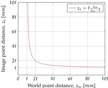
3.2 image formation 23 The length between the nearest and furthest out of focus image points, which are acceptably sharp, is called the depth of field. This is a phys-ical constraint, but it is less noticeable for objects further away.6 Equation3.9can be arranged as a translated hyperbola
zi=f zw
zw−f. (3.10)
It is obvious that∞> zw> f⇒f > zi> 2f, or ratherzilies between fand2f, ifzwlies between ∞and2f.7
Ifzwis sufficiently greater thanf, thenziwill be sufficiently close to f(Figure3.14). Acceptable sufficiency depends on the application. As an example, if f = 18 mmandzw = 1.8 m, thenzi = 18.18 mm; that is,zw=100f⇒zi=1.01f.
This behaviour is reminiscent of Figure 3.9, which illustrates how a lens’ focal length is measured. Indeed, light rays from world points that are far enough will appear to be collimated.
0 2f 4f 6f 8f 10f 2f 4f 6f 8f 10f f f
World point distance,zw[mm]
Image point distance, zi [ mm ] z i=fzw−fzw
Figure3.14: Thin lens behaviour using focal length multiples. If zw f⇒ zi ≈ f, then the whole image is nominally in focus on the focal plane; image focus is well defined. Also, the image plane is easily located if it coincides with the focal plane, such that it is at a distance,f, away from the lens.
Now, a lens focuses multiple light rays from one world point to one image point. When multiple images form, they overlap in the same position, increasing the image brightness, while keeping image sharp-ness (Figure3.15).
6 A lens’ aperture size and camera’s exposure time can be adjusted to increase depth of field, but the added latency may be unacceptable for real-time applications.
3.2 image formation 24
Figure3.15: Focused image formation using a lens.
In practice, lenses are cascaded for finer adjustment over f. Hence,f usually represents a lens system’s effective focal length.
3.2.2 Perspective Transform
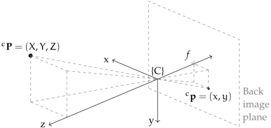
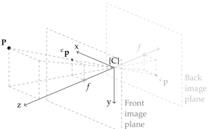
The relationship between a three-dimensional point cP = (X,Y,Z) and its image projection cp = (x,y) is modelled by the perspective transform (Figure3.16). x y z {C} cP= (X,Y,Z) cp= (x,y) f Back image plane Figure3.16: three-dimensional point projection through an equivalent
pin-hole.
The lens’ frame is attached with the camera’s frame, {C}. {C}’s origin coincides with the lens’ optical centre, or equivalent pinhole. It is obvious that Pandpare related via similarity of triangles,
x f = X Z, (3.11) y f = Y Z. (3.12)
It is more convenient to use the central projection model, which in-stead uses the front image plane. This plane is the reflection of the back image plane about the optical centre (Figure3.17).
3.2 image formation 25 x y z {C} cP cp cp f f Front image plane Back image plane
Figure3.17: Central projection model.
A non-inverted image is formed on the front image plane. This plane, from the optical centre’s point of view, is consistent with an observers’ point of view, such thatcPandcpmove in the same direction. 3.2.3 Normalised Image Plane
A common intermediate step betweencPandcpis to use normalised image coordinates [60, 74, 83], that is, image coordinates projected onto the plane at z=1(Figure3.18).
x y z {C} cP cp pn= (xn,yn) f z=1 Front image plane Normalised image plane
Figure3.18: Normalised image plane and coordinates. The normalised three-dimensional point ofcPis
¯pn= xn yn 1 = X/Z Y/Z Z/Z =CPn. (3.13)
3.2 image formation 26 It follows thatpnis scaled byfto obtaincp
c¯p= f 0 0 0 f 0 0 0 1 ¯pn. (3.14)
The normalised image coordinatepnis an unscaled intermediary for the theoretical image projection cp which isunobservable in the pres-ence of image distortions.
3.2.4 Geometric Lens Distortion
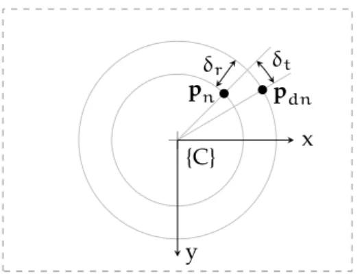
All lenses exhibit some sort of distortion that obfuscates the informa-tion on a projected image. The most prominent distorinforma-tions are radial and tangential distortions (Figure3.19, adapted [84]).
δr δt
pn pdn
x
y {C}
Figure3.19: Radial and tangential lens distortions on the normalised plane. Geometric distortions are systematic errors, which are easily corrected in software once parametrised. Let r2n := ||pn||2 = x2
n+y2n, then the distorted normalised image coordinate is
pdn= " xdn ydn # =pn+δr(xn,yn) +δt(xn,yn) (3.15) =pn+ k1r2n+k2r4n+k3r6n pn | {z } δr(xn,yn) + " 2p1xnyn+p2(r2n+2x2n) p1(r2n+2y2n) +2p2xnyn # | {z } δt(xn,yn) = 1+k1r2n+k2r4n+k3r6n pn + " 2p1xnyn+p2(r2n+2x2n) p1(r2n+2y2n) +2p2xnyn # =∆r(xn,yn)pn+δt(xn,yn). (3.16)
3.3 pixels, image sensors and digital images 27 This is the Brown-Conrady distortion model [85],8 parametrised by the low-order (normalised) radial and tangential distortion coefficients (k1,k2,k3,p1,p2). There are higher-order distortion coefficients, but low-order coefficients are enough for most applications [86,87]. Once the distortion coefficients are found, the inverse distortion can be computed to correct the distorted image [86,87], and the distorted normalised coordinate ¯pdnreplaces the normalised image coordinate
¯pn inEquation3.14, such that
c¯p= f 0 0 0 f 0 0 0 1 ¯pdn. (3.17)
3.3 Pixels, Image Sensors and Digital Images
The term pixel (px), or picture element, is a blanket term that is am-biguous without context. A pixel refers to, among others: a single element of an image sensor; a point sample of a digital image.
Specifically, single elements of an image sensor are differentiated us-ing the terms: photosite, sensor element, orsensel. A sensel is respon-sible for converting incoming photons, from the lens, into electrons. The quantity of electrons found, over an exposure time, relates to the intensity reported by a sensel.9 Then each sensel’s full colour value is demosaiced (or interpolated from adjacent sensels), based on the image sensor’s colour filter array.
A camera chip’s image sensor has a rectangular array, or pixel count, of W×H sensels. The distance between each sensel, or a sensel’s width or height, is called the pixel pitch, where ρw and ρh are the horizontal and vertical pitches, respectively.10These are usually spec-ified in µm/px [m/px]. Hence, the image sensor has a width and height ofWρw andHρh, respectively.
Unsurprisingly, the image sensor is modelled as a plane, which coin-cides with the back image plane. The sensor’s frame is called the pixel coordinate frame {X}, with u and v axes that are parallel to a camera frame’s x and y axes. Coordinates belonging to the pixel frame, or pixel coordinates, are measured in pixels.
On the front image plane, from the optical centre’s point of view, the pixel frame sits towards the upper left direction (Figure3.20).
8 Typically organised asEquation3.15(additive) orEquation3.16(multiplicative) in literature.
9 Reported intensity depends factors such as: quantum efficiency, lens aperture, shut-ter speed, fill factor, and analogue gain [4,81,88].
3.3 pixels, image sensors and digital images 28 (u0,v0) cp x y {C} u v {X} x cξ H-1
Figure3.20: Pixel coordinate frame on the front image plane.
The image plane intersection with the optical axis is called its princi-ple point.11 This point, with respect to {X}, is (u0,v0) and it is speci-fied in pixel coordinates. Pixel coordinates xp = (u,v) are found by quantising image coordinatescp= (x,y). In general,
x¯p= 1 ρw 0 u0 0 ρ1 h v0 0 0 1 c¯p. (3.18)
In practice, u,v /∈ Z>0 and must be rounded to a corresponding pixel, such thatu,v∈Z>0. Furthermore, pixel coordinates are stored digitally as point samples [89],12 which are commonly rendered on digital displays as squares (Figure3.21).
xp u v {X} 0 1 2 . . . W-1 0 1 2 ... H-1 Figure3.21: Square rendering of pixels.
By convention, a digital image’s first and last addressable pixel coor-dinates are usually(0,0)and(W−1,H−1), respectively.
11 The principle point is not necessarily the image sensor’s geometric centre, due to manufacturing misalignment [84].
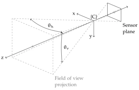
3.3 pixels, image sensors and digital images 29 3.3.1 Field of View
A camera only captures light rays in its field of view. The field of view is parametrised by its horizontal and vertical angles, subtended by the width and height of an image sensor, respectively (Figure3.22).
x y z {C} Sensor plane Field of view projection θh θv
Figure3.22: Vertical field of view. The horizontal field of view [4] is
tanθh 2 = W 2 ρw f θh=2tan−1 W 2 ρw f , (3.19)
and similarly, the vertical field of view θv =2tan−1
H 2ρh
f . (3.20)
The angles,θh andθv, decrease with increasingf, that is, a camera’s field of view will narrow due to magnification.
3.3.2 Sensor Spatial Resolution
Visual detail can only be captured reliably, or resolved, if it lies within a sensel’s field of view. The projection of a sensel’s size ρwρh sub-tended by its field of view atz= 1is called the sensel’s (normalised) spatial resolutions. These are
Pw 1 = ρw f , (3.21) Ph 1 = ρh f , (3.22)
3.4 intrinsic parameters 30 with units of(m/px)/m. The spatial x-y resolutions decrease, or im-prove, by increasingfand losing field of view.13
If, instead, field of view is specified, then, fromEquation3.19,14 Pw= 2 W tan θh 2 , (3.23) Ph = 2 Htan θv 2 . (3.24) 3.4 Intrinsic Parameters
GivenEquation3.17andEquation3.18, a complete camera model can be formed x¯p= 1 ρw 0 u0 0 ρh1 v0 0 0 1 f 0 0 0 f 0 0 0 1 ¯pdn = f ρw 0 u0 0 ρhf v0 0 0 1 ¯pdn =K ¯pdn, (3.25) where:
x¯p augmented pixel coordinate
K camera matrix
¯pdn augmented distorted normalised image coordinate.
The camera matrix Kand distortion coefficients are the intrinsic pa-rameters of a camera. These papa-rameters are determined by a camera calibration procedure.
The camera parametersf/ρwandf/ρh, or the pixel focal lengths [4], are lumped values, that is, f cannot be determined independently, unlessρworρh is known.
3.5 Extrinsic Parameters
A camera’s extrinsic parameters represents its relative pose with re-spect to a world coordinate frame, be it another camera, or the base of a robot arm on which it is mounted [18]. Once the relative pose is found, world coordinates can be referenced by the camera’s frame. 13 Overall spatial resolution depends on the cascaded sensor and lens spatial resolution.
Seehttp://photo.blogoverflow.com/2012/06/the-realities-of-resolution/.
3.6 summary 31 {W} x y z {C} x y z wP w cξ
Figure3.23: World coordinate frame. In general, this is
c¯P=c
wTw¯P=wcT−1 w¯P (3.26)
where:
c¯P augmented camera coordinate w
c T pose of the camera with respect to its world w¯P augmented world coordinate.
The pose matrix w
c T is the extrinsic parameter of a camera. Along with intrinsic parameters, extrinsic parameters can be determined by a camera calibration procedure.
3.6 Summary
A geometric camera model based on the pinhole camera has been presented. The result is a camera matrix which captures most of the important parameters. These are found using a suitable camera cali-bration procedure, after which image errors can be corrected.
4
K I N E C T C A M E R A C H A R A C T E R I S AT I O N
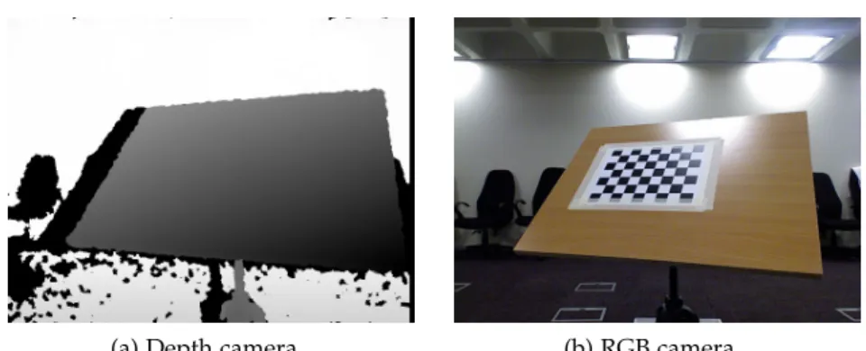
(a) Depth camera. (b) RGB camera.
Figure4.1: Kinect point of view.
The Kinect has a RGB and depth camera, anIRcamera and projector
pair, which outputs uncalibrated images shown in Figure 4.1. RGB camera models and calibration procedures are well known [74], but characterising the depth camera requires more attention.
Due to the Kinect’s proprietary nature, black box testing is neces-sary to characterise its performance and limitations. Disassembly is avoided, to prevent unintentional changes to its characteristics. Known characteristics about the RGB and depth camera, from various au-thors, are compared and discussed.
A corner-based calibration procedure is conducted using an assem-bled calibration rig and Herrera’s Kinect Calibration Toolbox (KCT), which runs joint nonlinear minimisation [60] and corrects for depth distortion. The procedure is followed by a comparison and discussion of results between various data sets and authors.
4.1 Components
A LED indicates the Kinect’s operational status (Figure4.2a). The IR
projector stands alone, emitting red light, followed by the RGB and
IR cameras, respectively. The RGB orIRcamera can be identified, by
physically covering either one’s view and observing a change on its data stream or captured image.
4.2 specifications 33
(a) Kinect operational. (b) IR projector filter.
Figure4.2: Kinect cameras and projector.
A blue lid covers theIRcamera’s lens, possibly anIRbandpass filter,
and the IR projector is shielded by a blue-tinted disk that becomes
opaque from a viewing angle onwards (Figure4.2b).
Figure4.3: Kinect product information.
The Kinect’s base reveals a model number,MODEL 1414 (Figure4.3).1 PatentsUS6483918andUS6775708are assigned to Microsoft Corpora-tion and implement techniques for robust data transmission.2 TheIR projector is a class one laser and conforms to the eye safety standard, IEC60825-1:2007-03.
4.2 Specifications
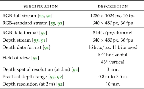
Microsoft published only the Kinect for Windows specifications [90]. Useful metrics are unspecified, such as pixel count, frame rate, depth resolution, and depth accuracy. Han et al. [55], OpenKinect’s protocol documentation [91], and OpenKinect’s imaging information [92] have provided some specifications. These are combined intoTable 4.1.
1 Model numbers are unmentioned by any known author.
4.3 depth camera characterisation 34
Table4.1: Kinect documented specifications.
specification description
RGB-full stream [55,91] 1280×1024 px,10 fps RGB-standard stream [55,91] 640×480 px,30 fps
RGB data format [55] 8 bits/px/channel
Depth stream [55,91] 640×480 px,30 fps Depth data format [91] 16 bits/px,11 bitsused
Field of view [55] 57° horizontal
43° vertical Depth spatial resolution (at2 m) [92] 3 mm Practical depth range [55,92] 0.8 mto3.5 m Depth resolution (at2 m) [92] 10 mm
Since spatial resolution scales linearly, the expected depth spatial res-olution at 1.0 mis1.5 mm.
The Kinect is capable of extending beyond the 3.5 mpractical depth range, but at the loss of depth resolution. The actual usable depth range is limited by the Kinect’s maximum accessible depth and an application’s depth error tolerance.
The expected uncompressed data sizes and rates for the three streams are calculated inTable4.2, signalling the required throughput.
Table4.2: Kinect image data sizes and data rates.
type data size (MB) data rate (MB/s)
RGB-full 3.932 39.32
RGB-standard 0.922 27.65
Depth 0.614 18.43
4.3 Depth Camera Characterisation 4.3.1 IR Speckle Pattern
Along with RGB and disparity images, the Kinect outputsIRimages.
These record the IR projector’s speckle pattern, which act as inter-mediaries in the depth processing pipeline, and do nothing more. Nonetheless, the IR images explain the some of the depth sensor’s