DOI10.1007/s10994-008-5055-9
Efficient approximate leave-one-out cross-validation
for kernel logistic regression
Gavin C. Cawley·Nicola L.C. Talbot
Received: 7 March 2007 / Revised: 24 March 2008 / Accepted: 29 March 2008 / Published online: 17 April 2008
Springer Science+Business Media, LLC 2008
Abstract Kernel logistic regression (KLR) is the kernel learning method best suited to
bi-nary pattern recognition problems where estimates of a-posteriori probability of class mem-bership are required. Such problems occur frequently in practical applications, for instance because the operational prior class probabilities or equivalently the relative misclassifica-tion costs are variable or unknown at the time of training the model. The model parameters are given by the solution of a convex optimization problem, which may be found via an efficient iteratively re-weighted least squares (IRWLS) procedure. The generalization prop-erties of a kernel logistic regression machine are however governed by a small number of hyper-parameters, the values of which must be determined during the process of model se-lection. In this paper, we propose a novel model selection strategy for KLR, based on a computationally efficient closed-form approximation of the leave-one-out cross-validation procedure. Results obtained on a variety of synthetic and real-world benchmark datasets are given, demonstrating that the proposed model selection procedure is competitive with a more conventionalk-fold cross-validation based approach and also with Gaussian process (GP) classifiers implemented using the Laplace approximation and via the Expectation Propaga-tion (EP) algorithm.
Keywords Model selection·Kernel logistic regression
1 Introduction
Kernel learning methods (see e.g. Müller et al.2001; Schölkopf and Smola2002; Shawe-Taylor and Cristianini 2004), such as the support vector machine (Boser et al. 1992; Cortes and Vapnik1995; Vapnik1998), kernel Fisher discriminant analysis (Mika et al.
1999,2003), kernel ridge regression (Saunders et al.1998) and kernel principal compo-nent analysis (Schölkopf et al.1997; Mika et al.2003), have attracted considerable interest
Editor: Olivier Chapelle. G.C. Cawley (
)·N.L.C. TalbotSchool of Computing Sciences, University of East Anglia, Norwich, NR4 7TJ, UK e-mail:[email protected]
in the machine learning community in recent years, due to a combination of mathematical tractability and state-of-the-art performance demonstrated over a wide range of benchmark datasets (e.g. Cawley and Talbot2003) and real-world applications (e.g. Brown et al.2000). Kernel learning methods generally aim to construct a linear model in a feature space induced by a positive definite Mercer kernel (Mercer1909). Depending on the choice of kernel, the feature space may be of high or even infinite dimension, while dealing with only finite di-mensional quantities, such as the kernel matrix giving the value of the kernel function for every pair of data points comprising the training sample. The richness of the feature space allows the construction of very complex, powerful models, however Tikhonov regularization (Tikhonov and Arsenin1977) has proved an effective means of capacity control, prevent-ing over-fittprevent-ing and optimizprevent-ing generalization. The linear nature of the underlyprevent-ing model means that the optimal model parameters are often given by the solution of a convex opti-mization problem (Boyd and Vandenberghe2004), with a single global optimum, for which efficient algorithms exist. The generalization properties of kernel methods however tend to be heavily dependent on the values of a small number of hyper-parameters, including regularization parameters (Tikhonov and Arsenin1977) and parameters defining the kernel function (Chapelle et al.2002). The search for the optimal values of these hyper-parameters is a process known as model selection. Unfortunately the model selection criteria for kernel learning methods are not generally unimodal, and so this paper is concerned with efficient search methods for finding a locally optimal set of hyper-parameter values.
The most common approach to model selection aims to minimize some form of cross-validation (Stone1974) estimate of an appropriate model selection criterion, for example the misclassification rate or perhaps the cross-entropy in the case of a statistical pattern recognition problem. Under ak-fold cross-validation scheme, the available data are divided intokdisjoint subsets. A model is then trained onk−1 of these subsets and the model selection criterion evaluated on the unused subset. This procedure is then repeated for allk combinations ofk−1 subsets. Thek-fold cross-validation estimate for the model selection criterion is then simply the mean of the model selection criterion computed over the unused subset in each fold. Cross-validation makes good use of the available data as all data are used as both training and test data. The most extreme form ofk-fold cross-validation, in which each subset consists of a single training pattern is known as leave-one-out cross-validation (Lachenbruch and Mickey1968). An attractive property of leave-one-out cross-validation for model selection purposes is that it provides an almost unbiased estimate of generaliza-tion performance (Luntz and Brailovsky1969). The regularization and kernel parameters can then be tuned via minimization of the leave-one-out error using standard optimization techniques, such as the Nelder-Mead simplex algorithm.
Unlike kernel methods based on a least-squares training criterion, exact leave-one-out cross-validation of kernel logistic regression cannot be performed efficiently in closed-form. However in this paper, we propose a useful approximation, based on exact leave-one-out cross-validation of the quadratic approximation to the regularized training criterion obtained during the final iteration of the IRWLS training algorithm. This extends an existing efficient leave-one-out method for kernel Fisher discriminant analysis (Cawley and Talbot2003) to be adapted for computationally efficient model selection for a family of kernel learning meth-ods, including kernel logistic regression. The approximation is also shown to be equivalent to taking a single Newton step to minimize the reduced training criterion in each iteration of the leave-one-out procedure, starting from the optimal parameters for a model fitted to the entire training sample (see AppendixA).
The remainder of this paper is structured as follows: Sect.2introduces the kernel logistic regression model and introduces the notation used throughout. Section3proposes a simple
model selection procedure for KLR based on an efficient, closed-form approximation of the leave-one-out andk-fold cross-validation estimates of the test cross-entropy. Section4 com-pares model selection procedures based on approximate leave-one-out and conventional k-fold cross-validation. Results are also obtained for expectation-propagation based Gaussian process classifiers, providing a state-of-the-art baseline for comparison purposes. Results presented in Sect.4demonstrate that the approximate leave-one-out cross-validation pro-cedure is competitive with the alternative propro-cedures, at a vastly reduced computationally expense. Finally, the work is summarized and conclusions drawn in Sect.5.
2 Kernel logistic regression
In this section, we provide a brief overview of the kernel logistic regression (KLR) model, and introduce the notation used throughout. In an off-line statistical pattern recognition prob-lem, we are given labeled training data,
D= {(xi, ti)}i=1, xi∈X⊂Rd, ti∈ {0,1},
on which a decision rule is trained to discriminate between examples belonging to positive and negative classes, where xirepresents a vector ofdinput variables describing theith ex-ample, andtiindicates the class of theithexample, whereti=1 if the example belongs to the positive classC+andti=0 if it belongs to the negative classC−. Kernel logistic regression aims to construct a familiar linear logistic regression model in a high-dimensional feature space induced by a Mercer kernel, giving rise to a non-linear form of logistic regression, i.e.
logit{y(x)} =w·φ(x)+b, where logit{p} =log
p 1−p
,
w is a vector of model parameters,φ(·)represents a non-linear transformation of the input
vectors. Equivalently, we could write
y(x)= 1
1+exp{−w·φ(x)−b}.
The logit link function constrains the output of the model to lie in the range[0, 1]. Rather than specifying the transformationφ:X →F directly, it is implied by a Mercer kernel,
K:X ×X →R, which evaluates the inner product between the images of vectors in the
feature space,F,
K(x,x)=φ(x)·φ(x).
For the interpretation of the kernel function as an inner product in a fixed feature space to be valid, the kernel must obey Mercer’s condition (Mercer1909), i.e. the kernel or Gram matrix, K= [kij=K(xi,xj)]i,j=1, must be positive (semi)-definite. The kernel most
com-monly used in practical applications of kernel learning methods is the squared exponential, or radial basis function (RBF), kernel,
K(x,x)=exp{−θx−x2}, (1) whereθis a kernel parameter controlling the sensitivity of the kernel. Interpreting the output of the kernel logistic regression model as an estimate of the a-posteriori probability of class
membership, then provided the data represent an i.i.d. (independent and identically distrib-uted) sample from a Bernoulli distribution conditioned on the input variables, the likelihood of the training data is given by
L= i=1 yti i[1−yi] 1−ti,
whereyi=y(xi). The optimal vector of model parameters, w, is found by minimizing a cost function representing the regularized (Tikhonov and Arsenin1977) negative log-likelihood of the training data, in this case known as the cross-entropy,
E=1 2w 2−γ 2 i=1
[tilog{yi} +(1−ti)log{1−yi}], (2) whereγ is a regularization parameter controlling the bias-variance trade-off (Geman et al.
1992). The representer theorem (Kimeldorf and Wahba1971; Schölkopf et al.2002) states that the solution to an optimization problem of this nature can be written in the form of a linear combination of the training patterns, i.e.
w=
i=1
αiφ(xi), which implies that
logit{y(x)} =
i=1
αiK(xi,x)+b and w2=αKα,
whereα=(α1, α2, . . . , α)is a vector of dual model parameters. The benefit of the
“ker-nel trick” then becomes apparent; it allows us to construct powerful linear models in very high (potentially infinite) dimensional feature spaces using mathematics involving only fi-nite quantities, such as the×Gram matrix.
2.1 Iteratively re-weighted least squares training procedure
The objective function for a wide range of kernel learning methods, including kernel logistic regression, can be written in the form,
E=1 2w 2+γ i=1 c(yi, ti) (3)
wherec(·,·)is a convex loss function, in this case the negative log-likelihood assuming a Bernoulli trial,c(y, t )= −[tlogy+(1−t )log(1−y)]. A closed form expression for the minimum of the objective function (3) is not immediately apparent, and so it is most easily minimized via an iteratively re-weighted least-squares (IRWLS) procedure, commonly used in training conventional logistic regression models and radial basis function (RBF) networks (Nabney1999). Letzirepresent the output of the kernel machine for theithtraining pattern, prior to the non-linear transform,
zi=
j=1
In the case of kernel logistic regression,zirepresents the log-odds ratio. The first and second derivatives of the loss, with respect tozi, are then given by
∂ci ∂zi =yi−ti and ∂2ci ∂z2 i =yi(1−yi),
whereci=c(yi, ti). As we are interested only in minimizing the convex loss function, we substitute a weighted least-squares criterion, providing a local approximation ofcionly up to some arbitrary constant,C, i.e.
qi=βi
2[ηi−zi]
2≈c(yi, ti)+C.
Clearly, we require the curvature ofqi andci, with respect tozi, to be identical atzi, and therefore ∂2qi ∂z2 i =∂2ci ∂z2 i ⇒ βi=yi(1−yi).
We also require the gradient ofqi, with respect tozi, to match that ofci, such that ∂qi
∂zi = −βi[ηi−zi] = ∂ci
∂zi ⇒ ηi=zi− yi−ti yi(1−yi).
The original objective function (2), can then be solved iteratively, alternating updates of the dual parameters,(α, b), via a regularized weighted least-squares loss function,
Lσ=1 2w 2+γ 2 i=1 βi[ηi−zi]2, (4) and updates of the weighting coefficients, β=(β1, β2, . . . , β), and targets, η=(η1, η2,
. . . , η). In the case of kernel logistic regression, the update formulae are: βi=yi(1−yi) and ηi=zi− yi−ti
yi(1−yi). (5) The weighted least-squares problem (4) can also be solved via a system of linear equations, with a computational complexity ofO(3) operations, as follows: Minimizing (4) can be recast in the form of a constrained optimization problem (Suykens et al.2002a),
minJ =1 2w 2+γ 2 i=1 βiε2i (6) subject to ηi=w·φ(xi)+b+εi, ∀i∈ {1,2, . . . , }. (7) The primal Lagrangian for this optimization problem gives the unconstrained minimization problem, L=1 2w 2+γ 2 i=1 βiεi2− i=1
whereα=(α1, α2, . . . , α)∈Ris a vector of Lagrange multipliers. The optimality
condi-tions for this problem can be expressed as follows:
∂L ∂w=0 ⇒w= i=1 αiφ(xi), (8) ∂L ∂b =0 ⇒ i=1 αi=0, (9) ∂L
∂εi =0 ⇒αi=βiγ εi, ∀i∈ {1,2, . . . , }, (10) ∂L
∂αi =0 ⇒w·φ(xi)+b+εi−ηi=0, ∀i∈ {1,2, . . . , }. (11) Using (8) and (10) to eliminate w andε=(ε1, ε2, . . . , ε), from (11), we find that
j=1 αjφ(xj)·φ(xi)+b+ αi γ βi =ηi, ∀i∈ {1,2, . . . , }. (12) Noting that K(x,x)=φ(x)·φ(x), the system of linear equations can be written more concisely in matrix form as
K+γ1B 1 1 0 α b = η0 , (13)
where K= [kij=K(xi,xj)]i,j=1and B=diag{β− 1
1 , β−
1 2 , . . . , β−
1
}. The optimal parameters for the kernel machine can then be obtained with a computational complexity ofO(3) oper-ations. Note that the iteratively re-weighted least-squares (IRWLS) procedure is equivalent to the application of Newton’s method. We present the learning algorithm in terms of IR-WLS here as the proposed approximate leave-one-out method is an extension of an existing exact method for weighted least-squares models.
2.2 Efficient implementation via Cholesky decomposition
A more efficient training algorithm can be obtained, taking advantage of the special structure of the system of linear equations. The system of linear equations (13) to be solved during each step of the iteratively re-weighted least squares procedure is given by,
M 1 1 0 α b = η0 , (14)
where M=K+γ−1B. Unfortunately the matrix on the left-hand side is not positive
def-inite, and so we cannot solve this system of linear equations directly using the Cholesky decomposition (Golub and Van Loan1996). However, the first row of (14) can be re-written as
Rearranging (15), we see thatα=M−1(η−1b), using this result to eliminateα, the second
row of (14) can be written as,
1M−11b=1M−1η. (16)
The system of linear equations (14) can be then be solved by first solving two positive definite linear systems
Mξ=1 and Mζ=η, (17)
and then updating the model parameters of the kernel logistic regression machine as follows:
b=1
ζ
1ξ and α=ζ−ξb.
The two systems of linear equations (17) can be solved efficiently using the Cholesky de-composition of M=RR, where R is the upper triangular Cholesky factor of M (Suykens
et al.2002b). Note that the computational complexity of the Cholesky decomposition is
O(3), but that of the back-substitution used in solving the two systems of linear equations
is onlyO(2)operations. As a result, the Cholesky decomposition is both computationally
efficient as well as numerically more robust (Golub and Van Loan1996).
3 Cross-validation based model selection strategies
The simplest form of model selection criterion typically partitions the available data into training, validation and test sets. The training set is used to determine the optimal values of the model parameters, an appropriate performance measure is evaluated over the validation or hold-out set in order to optimize the hyper-parameters and the test set is used to obtain an unbiased estimate of generalization performance. If data is relatively scarce, a cross-validation procedure is often used (Stone1974). Under ak-fold cross-validation strategy, the data are partitioned intoksubsets of approximately equal size. Models are then trained on each of thekcombinations ofk−1 subsets, in each case the performance of the model is estimated using the remaining subset not forming part of the training data for that model. The cross-validation estimate of a given performance metric is simply the mean of the perfor-mance in each fold of the cross-validation procedure. Cross-validation clearly makes better use of the available data as every pattern is used as both a training and a test pattern. The most extreme form of cross-validation, in which each subset contains only a single pattern, is known as leave-one-out cross-validation (Lachenbruch and Mickey1968). Leave-one-out cross-validation is often used in model selection, partly as it is known to be approximately unbiased (Luntz and Brailovsky1969), but also because it can be implemented very effi-ciently in the case of linear regression, least-squares kernel learning methods (Allen1974; Cook and Weisberg1982; Weisberg1985; Cawley and Talbot2003,2004b; Bo et al.2006; Rasmussen and Williams2006) andk-nearest neighbor methods, or approximated efficiently in the case of the support vector machine (Chapelle et al.2002). In this paper, in addition to investigating conventional cross-validation based model selection strategies, we also pro-pose an approximate leave-one-out cross-validation method for kernel logistic regression based on existing efficient methods for least-squares kernel learning methods, the method presented here being a greatly refined version of the method briefly outlined in Cawley and Talbot (2004a). However, the approach is quite general, and can easily be applied to any kernel regression method with a convex loss function,c(·,·).
3.1 Approximate leave-one-out cross-validation
The optimal values for the parameters of a kernel regression model are iteratively determined via a sequence of weighted least-squares optimization problems. It is well known that leave-one-out cross-validation of least-squares models can be performed very efficiently in closed form (Cook and Weisberg1982; Weisberg1985; Green and Silverman1994; Cawley and Talbot2003; Cawley and Talbot 2004b). These methods can be extended to provide an approximate leave-one-out cross-validation method for kernel regression methods with an arbitrary loss, via exact leave-one-out cross-validation of the quadratic approximation (4) of the true loss minimized in the final iteration of the IRWLS training procedure (Green and Silverman1994; Cawley and Talbot2004a). The matrix on the left-hand side of (13) can be decomposed into block-matrix representation, as follows:
K+γ−1B 1 1 0 = c11 c1 c1 C1 =C. (18)
Let[α(−i);b(−i)]represent the parameters of the kernel machine during theithiteration of
the leave-one-out cross-validation procedure, then in the first iteration, in which the first training pattern is excluded,
α(−1)
b(−1)
=C−11[η2, . . . , η,0].
The leave-one-out prediction for the first training pattern is then given by,
ˆ z(1−1)=c1 α (−1) b(−1) =c1C−11 [η2, . . . , η,0].
Considering the last equations in the system of linear equations (13), it is clear that [c1C1][α1, . . . , α, b]= [η2, . . . , η,0], and so
ˆ
z(1−1)=c1C−11 [c1C1][α, b]=c1C−11 c1α1+c1[α2, . . . , α, b].
Noting, from the first equation in the system of linear equations (13), thatη1=c11α1+ c1[α2, . . . , α, b], thus
ˆ
z(1−1)=η1−α1(c11−c1C−11 c1).
Finally, via the block matrix inversion lemma,
c11 c1 c1 C1 −1 = κ−1 −κ−1c1C−11 C−11 +κ−1C−11 c1c1C−11 −κ−1C−11 c1 , (19) whereκ=c11−c1C− 1
1 c, and noting that the system of linear equations (13) is insensitive
to permutations of the ordering of the equations and of the unknowns, we have that,
ˆ
zi(−i)=ηi− αi
C−ii1. (20)
This means that, assuming the system of linear equations (13) is solved via explicit inversion of C, an approximate leave-one-out cross-validation estimate of the test loss (22) can be
evaluated using information already available as a by-product of training the least-squares support vector machine on the entire dataset. This approximation is based on the assumption that the parameters of the quadratic approximation of the regularized loss function,β and
ηare essentially unchanged during the leave-one-out cross-validation procedure (c.f. Green and Silverman1994). Essentially we substitute a leave-one-out cross-validation of the model using the quadratic approximation for a leave-one-out cross-validation using the true loss. Alternatively, as described in AppendixA, we can view the approximation as taking a single Newton step of the reduced training criterion in each fold of the leave-one-out procedure, starting from the vector of model parameters minimizing the regularized loss on the entire training sample.
3.2 Efficient implementation via Cholesky factorization
The approximate leave-one-out cross-validation estimator for kernel logistic regression is described by (20). The coefficients of the kernel expansion, α, can be found efficiently, via iteratively re-weighted least squares based on Cholesky factorization, as described in Sect.2.2. However we must also determine the diagonal elements of C−1in an efficient manner. Using the block matrix inversion formula, we obtain
C−1= M 1 1 0 −1 = M−1+M−11S−1M1M−1 −M−11S−1M −S−1M1M−1 S−1 M
where M=K+γ−1B and SM= −1M−11= −1ξ is the Schur complement of M. The inverse of the positive definite matrix, M, can be computed efficiently from its Cholesky factorization, via theSYMINV algorithm (Seaks1972), for example using the LAPACK (Anderson et al.1999) routineDTRTRI. Let R= [rij]n
i,j=1be the lower triangular Cholesky factor of the positive definite matrix M, such that M=RR. Furthermore, let
S= [sij]ni,j=1=R−1, wheresii= 1
rii andsij= −sii i−1
k=1 rikskj,
represent the (lower triangular) inverse of the Cholesky factor. The inverse of M is then given by M−1=SS. In the case of efficient approximate leave-one-out cross-validation
of kernel logistic regression machines, we are principally concerned only with the diagonal elements of M−1, given by Mii−1= i j=1 sij2 ⇒ Cii−1= i j=1 sij2+ ξ 2 i SM , ∀i∈ {1,2, . . . , }.
The computational complexity of the basic training algorithm isO(3) operations, being
dominated by the evaluation of the Cholesky factor. However, the computational complexity of the analytic approximate leave-one-out cross-validation approximation, when performed as a by-product of the training algorithm, is onlyO()operations. The computational ex-pense of the leave-one-out cross-validation procedure therefore rapidly becomes negligible as the training set becomes larger.
Note that the proposed approximate leave-one-out cross-validation procedure is quite general, and can be applied to kernel regression machines with an essentially arbitrary con-vex loss, for instance kernel Poisson regression (Cawley et al.2007). The support vec-tor machine (Boser et al.1992; Cortes and Vapnik1995) can also be trained in primal
form via Newton’s method (Chapelle2007), where the approximate leave-one-out cross-validation method given here is equivalent to the span bound (Vapnik and Chapelle2000; Chapelle et al.2002). It should be noted, however, that the proposed leave-one-out cross-validation method is not suitable for large scale applications in its current form, due to the computational complexity ofO(3) operations. For large scale applications, sparse algo-rithms, such as the import vector machine (Zhu and Hastie2005), could be used. However, if a sparse set of basis vectors has been identified, an approximate leave-one-out cross-validation method for sparse kernel logistic regression would be feasible based on the cor-responding approach for sparse least-squares kernel machines (Cawley and Talbot2004a,
2004b).
3.3 Optimization strategies
In practical applications of kernel learning methods the hyper-parameters are most often se-lected via a simple grid-based search method, in which the model selection criterion is evalu-ated at a set of points, forming a regular grid with even spacing, normally over a logarithmic scale. An improved hierarchical grid search procedure repeats this process, each time using a refined grid centered on the best solution found at the previous scale. However, grid-search procedures rapidly become computationally unfeasible as the number of hyper-parameters to be optimized grows larger than only two or three. However, if the model selection strategy is a relatively smooth function of the hyper-parameters, the Nelder-Mead simplex optimiza-tion algorithm (Nelder and Mead1965), as implemented by thefminsearchroutine of the MATLAB optimization toolbox, provides a simple and efficient alternative, as long as the number of hyper-parameters remains relatively small (less than about ten). For problems with a larger vector of hyper-parameters, gradient-based methods are likely to be more ef-ficient, for instance conjugate-gradient methods, as implemented by thefminuncroutine of the MATLAB optimization toolbox, or scaled conjugate gradient optimization (Williams
1991). AppendixB provides the derivation of gradient information with a computational complexity ofO(3+d2)operations, whered is the number of kernel parameters. Note that for the Gaussian process classifier based on the Laplace approximation, the gradient of the marginal likelihood, with respect to the parameters of the covariance function, can be evaluated with a complexity ofO(d2) operations (provided the inverse of the
covari-ance matrix is available as a by-product of fitting the model). The computational expense of model selection for LOO-KLR and L-GPC can thus be expected to exhibit similar scaling. However, when fitting models with many hyper-parameters there is a danger of over-fitting the model selection criterion, and so the addition of a regularization term to the selection criterion may be beneficial (Cawley and Talbot2007). It should be noted however, that the use of gradient-based methods does not necessitate the analytic computation of gradient in-formation (c.f. Bo et al.2006) as the required partial derivatives can also be approximated by the method of finite-differences, albeit with an increased complexity ofO(d3)operations.
3.4 Model selection for Gaussian process classifiers
An estimate of the leave-one-out cross-validation loss is also available as a by-product of fit-ting a Gaussian process classifier using the Expectation Propagation algorithm (Minka2001; Rasmussen and Williams2006). This approach is equivalent to the mean-field methods in-troduced by Opper and Winther (2000). Sundararajan and Keerthi (2001) present a leave-one-out cross-validation procedure for hyper-parameter selection in Gaussian process re-gression, also discussed in Rasmussen and Williams (2006). The Gaussian process classifier
based on the Laplace approximation (Williams and Barber1998) also uses a model selection criterion, in this case the marginal likelihood, evaluated using a quadratic approximation to the regularized loss function. The model selection process for Gaussian process classifiers under the Laplace approximation thus bears some similarities with the proposed approxi-mate leave-one-out cross-validation method.
4 Results
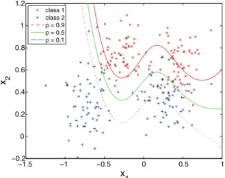
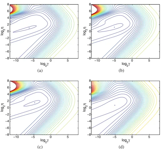
We begin by investigating the accuracy of the approximate leave-one-out method using Rip-ley’ssyntheticdata. Figure1shows a kernel logistic regression model of this dataset, using an isotropic radial basis function kernel. Figure2shows contour plots of the cross-entropy loss for a kernel logistic regression model of Ripley’ssyntheticdata, using an isotropic radial basis function kernel, computed using the proposed approximate leave-one-out method, exact leave-one-leave-one-out, 10-fold cross-validation and the test loss as a function of the hyper-parameters. It is clear that the approximate leave-one-out loss behaves in a similar manner to the exact leave-one-out loss, without being exactly identical. Most importantly, the minimum of all three estimates of the true loss are in accordance with the loss computed over the independent test set. Note that the loss is a smooth function of the hyper-parameters and so is well suited to automated model selection using standard non-linear optimization methods. Figure3shows the exact and approximate leave-one-out cross-entropy loss as a function of each of the hyper-parameters, holding the other constant at its optimal value. The approximate leave-one-out estimator is clearly of sufficient accuracy for model selec-tion purposes, but would not be suitable for performance evaluaselec-tion, except for well-tuned models. Note also that cross-validation based model selection criteria are not necessarily unimodal.
Next, we present experimental results demonstrating the accuracy and efficiency of the proposed approximate leave-one-out cross-validation model selection procedure for kernel logistic regression. Table1shows a comparison of the error rates of kernel logistic regres-sion, using the proposed approximate leave-one-out cross-validation based model selection process, and a variety of other state-of-the-art statistical pattern recognition algorithms over the suite of thirteen public domain benchmark datasets used in the study by Mika et al.
Fig. 1 Kernel logistic regression model of Ripley’ssynthetic
data, with isotropic radial basis function kernel and approximate leave-one-out cross-validation based model selection
Fig. 2 Contour plots of (a) the approximate leave-one-out cross-entropy loss, (b) the exact leave-one-out loss, (c) the 10-fold cross-validation loss and (d) the test set loss for thesyntheticbenchmark, for a kernel logistic regression model, as a function of the regularization parameter,γ, and the kernel parameter,η. The minimum loss is indicated by a cross,+
(2000). The same set of 100 random partitions of the data (20 in the case of theimageand
splicebenchmarks) to form training and test sets used in that study are also used here. In the case of the LOO-KLR, KLR, EP-GPC and LOO-KFD algorithms, model selection is performed independently for each realization of the dataset, such that the standard errors reflect the variability of both the training algorithm and the model selection procedure with changes in the sampling of the data. For the LOO-KLR and KLR methods, model selec-tion was performed via the Nelder-Mead simplex algorithm (Nelder and Mead1965). The isotropic squared exponential (RBF) kernel is used for all kernel learning methods, includ-ing the L-GPC and EP-GPC, chosen due to their state-of-the-art performance and similar structure.
Table2shows the model selection time for leave-one-out and 10-fold cross-validation based kernel logistic regression (LOO-KLR and KLR respectively) and expectation propa-gation and Laplace approximation based Gaussian process classifiers (EP-GPC and L-GPC). Table3shows the average amount of information about the test set labels in excess of
pre-Ta b le 1 Error rates of v arious state-of-the-art classifiers o v er thirteen benchmark d atasets, (LOO-KLR) k ernel logistic re gression using the proposed lea v e-one-out cross-v alidation m odel selection p rocedure, (KLR) k ernel logistic re gression with con v entional 10-fold cross-v alidation b ased model selection, Gauss ian p rocess classifier implemented via the Laplace approximation and expectation p ropagation algorithm (L-GPC and EP-GPC respecti v ely), (LOO-KFD) k ernel Fisher discriminant with lea v e-one-out cross-v alidation b ased model selection p rocedures (Ca w le y and T albot 2003 ), (SVM) support v ector machine (Boser et al. 1992 ; C ortes and V apnik 1995 ) and (KFD) k ernel F isher discriminant classifier (Mika et al. 1999 ). The results for m odels SVM and KFD are tak en from the study by Mika et al. ( 2000 ). The results for m odel L OO-KFD are tak en from C aw le y and T albot ( 2003 ). The results for the L-GPC and EP-GPC were obtained u sing the G PML M A TLAB toolbox accompan ying the book by Rasmussen and W illiams ( 2006 ). The results for each method are p resented in the form o f the mean error rate o v er test d ata for 100 realizations of each dataset (20 in the case o f the ima ge and splice datasets), along with the associated standard error . The b est results are sho wn in boldf ace and the second best in italics (without implication o f sta tistical significance) Dataset L OO-KLR K LR L-GPC E P-GPC L OO-KFD S VM KFD Banana 10 . 6 ± 0 . 05 10.5 ± 0.05 10 . 4 ± 0 . 05 10 . 4 ± 0 . 05 10 . 4 ± 0 . 04 11 . 5 ± 0 . 07 10 . 8 ± 0 . 05 Breast cancer 26 . 6 ± 0 . 47 26 . 5 ± 0 . 49 26 . 5 ± 0 . 48 26 . 5 ± 0 . 49 26 . 3 ± 0 . 42 26.0 ± 0 . 47 25 . 8 ± 0 . 46 Diabetes 23 . 4 ± 0 . 18 23 . 5 ± 0 . 16 23 . 3 ± 0 . 18 23 . 3 ± 0 . 18 23 . 1 ± 0 . 18 23 . 5 ± 0 . 17 23.2 ± 0.16 Flare solar 34 . 3 ± 0 . 17 34 . 2 ± 0 . 16 34 . 2 ± 0 . 18 34 . 2 ± 0 . 21 34 . 2 ± 1 . 16 32 . 4 ± 0 . 18 33.2 ± 0.17 German 23.5 ± 0.21 23.5 ± 0.21 23 . 4 ± 0 . 21 23 . 4 ± 0 . 21 23 . 6 ± 0 . 20 23 . 6 ± 0 . 21 23 . 7 ± 0 . 22 Heart 1 6 . 6 ± 0 . 31 16 . 6 ± 0 . 31 16 . 4 ± 0 . 28 16 . 7 ± 0 . 29 15 . 9 ± 0 . 35 16.0 ± 0.33 16 . 1 ± 0 . 34 Image 3 . 1 ± 0 . 13 3 . 1 ± 0 . 11 2 . 8 ± 0 . 10 2 . 8 ± 0 . 12 4 . 0 ± 0 . 06 3.0 ± 0.06 3 . 3 ± 0 . 06 Ringnorm 1 . 6 ± 0 . 02 1 . 6 ± 0 . 01 5 . 9 ± 0 . 08 4 . 4 ± 0 . 06 1 . 4 ± 0 . 08 1 . 7 ± 0 . 01 1.5 ± 0.01 Splice 1 1 . 2 ± 0 . 18 11 . 2 ± 0 . 17 12 . 3 ± 0 . 18 11 . 6 ± 0 . 18 10.8 ± 0.07 10 . 9 ± 0 . 07 10 . 5 ± 0 . 06 Thyroid 4.3 ± 0.21 4 . 7 ± 0 . 21 4 . 5 ± 0 . 21 4 . 4 ± 0 . 22 4 . 5 ± 0 . 20 4 . 8 ± 0 . 22 4 . 2 ± 0 . 21 T itanic 2 2 . 6 ± 0 . 10 22 . 6 ± 0 . 09 22 . 6 ± 0 . 13 22 . 6 ± 0 . 13 22 . 3 ± 0 . 12 22.4 ± 0.10 23 . 2 ± 0 . 20 T w onorm 2 . 9 ± 0 . 03 2 . 9 ± 0 . 03 3 . 1 ± 0 . 04 3 . 1 ± 0 . 03 2.7 ± 0.02 3 . 0 ± 0 . 02 2 . 6 ± 0 . 02 W av eform 9.9 ± 0.04 9.9 ± 0.04 10 . 0 ± 0 . 04 10 . 1 ± 0 . 05 9 . 7 ± 0 . 04 9.9 ± 0.04 9.9 ± 0.04
Fig. 3 Plot of the approximate and exact leave-one-out cross-entropy loss, as a function of (a) the regular-ization parameter,γ, with the kernel parameter,η, held at its optimal value and (b) the kernel parameter, with the regularization parameter held at its optimal value
Table 2 Model selection time for kernel logistic regression models with leave-one-out and 10-fold cross-validation based model selection (LOO-KLR and KLR respectively) and Gaussian process classifiers based on the Laplace approximation and expectation propagation (L-GPC and EP-GPC respectively) over thirteen benchmark datasets
Dataset Selection time (seconds)
LOO-KLR KLR L-GPC EP-GPC Banana 37.5±1.231 199.1±7.995 44.6±0.587 916.9±20.51 Breast cancer 5.4±0.210 28.7±1.030 16.0±0.269 126.2±1.919 Diabetes 37.9±0.939 201.9±5.803 111.5±1.746 1129.2±22.10 Flare solar 90.1±4.703 429.6±22.33 273.7±3.610 3108.9±75.08 German 99.5±2.687 531.8±12.03 566.9±6.853 3760.4±67.04 Heart 3.1±0.092 18.2±0.645 18.5±0.227 116.6±2.177 Image 832.6±94.82 4537.5±168.0 3643.6±378.3 25764.9±2314 Ringnorm 60.9±1.948 359.9±6.555 216.8±3.825 1544.7±43.35 Splice 237.4±10.84 1325.7±74.08 4054.2±122.72 12653.7±1480 Thyroid 5.2±0.348 21.6±0.839 9.0±0.278 133.4±4.049 Titanic 3.3±0.192 11.5±0.447 5.1±0.053 83.8±2.669 Twonorm 46.7±1.218 270.0±7.240 245.6±3.722 1302.0±45.05 Waveform 46.5±0.998 260.2±6.509 222.0±2.263 1145.2±35.38
dictions based on the prior class frequencies,
I=1+1 n
n
i=1
tilog2yi+(1−ti)log2(1−yi)
wherenis the number of test patterns. This statistic provides a measure of the accuracy of the predictions of a-posteriori probability obtained from a model (note that it is closely related to the cross-entropy).
Table 3 Mean target information for kernel logistic regression models with leave-one-out and 10-fold cross-validation based model selection (LOO-KLR and KLR respectively) and Gaussian process classifier based on the Laplace approximation and expectation propagation (L-GPC and EP-GPC respectively) over thirteen benchmark datasets
Dataset Information (bits)
LOO-KLR KLR L-GPC EP-GPC Banana 0.648±0.002 0.653±0.001 0.647±0.001 0.655±0.001 Breast cancer 0.222±0.007 0.223±0.007 0.228±0.006 0.227±0.007 Diabetes 0.306±0.003 0.306±0.003 0.312±0.003 0.311±0.003 Flare solar 0.172±0.002 0.172±0.002 0.174±0.002 0.174±0.002 German 0.294±0.004 0.296±0.004 0.297±0.004 0.298±0.004 Heart 0.421±0.007 0.424±0.007 0.425±0.007 0.421±0.008 Image 0.876±0.005 0.875±0.005 0.671±0.010 0.881±0.004 Ringnorm 0.930±0.002 0.932±0.001 0.613±0.001 0.757±0.003 Splice 0.613±0.004 0.613±0.004 0.532±0.001 0.589±0.003 Thyroid 0.806±0.023 0.837±0.012 0.708±0.012 0.858±0.006 Titanic 0.182±0.011 0.242±0.004 0.257±0.002 0.256±0.002 Twonorm 0.885±0.001 0.886±0.001 0.872±0.001 0.880±0.001 Waveform 0.675±0.001 0.675±0.001 0.654±0.001 0.668±0.001
The use of multiple training/test partitions allows an estimate of the statistical signifi-cance of differences in performance between algorithms to be computed. Letxˆandyˆ rep-resent the means of the performance statistic for a pair of competing algorithms, andexand eythe corresponding standard errors, then thezstatistic is computed as
z=yˆ− ˆx e2
x+ey2 .
Thez-score can then be converted to a significance level via the normal cumulative distrib-ution function, such thatz=1.64 corresponds to a 95% significance level. All statements of statistical significance in the remainder of this section refer to a 95% level of significance. Comparison of leave-one-out and 10-fold cross-validation based model selection strategies for kernel logistic regression reveals that the performance of both model selection strategies are very similar in terms of mean error rate. None of the differences in mean error rate for the two algorithms, shown in Table1, are statistically significant at the 95% level. The estimates of a-posteriori probability obtained using these approaches are generally very similar, with k-fold cross-validation being statistically superior on only two benchmarks (BANANAand
TITANIC). The kernel Fisher discriminant classifier appears to perform better than KLR or GPC models in terms of error rate, however it should be noted that the KFD classifier does not attempt to estimate the conditional probability of class membership, and so has an easier learning task, that concentrates more strongly on the decision boundary. Table2also shows that the approximate leave-one-out cross-validation based model selection is significantly less expensive, being approximately five times faster than the 10-fold cross-validation based approach, even though the latter had been extensively optimized (e.g. to prevent redundant evaluation of the kernel matrix). The computational complexity of the L-GPC, EP-GPC, KLR and LOO-KLR procedures are allO(3)operations (being dominated by the cost of
fitting the initial model), so the model selection times essentially differ only by a constant factor for a given dataset.
The Gaussian process classifier, based on the expectation propagation algorithm (EP-GPC) with hyper-parameters selected so as to maximize the marginal likelihood, represents
the state-of-the-art model having the same basic structure and design goals as kernel logistic
regression (see e.g. Rasmussen and Williams2006). The EP-GPC therefore provides a stern test of the proposed model selection algorithm. The Gaussian process classifier based on the Laplace approximation (L-GPC) is also relevant; like the LOO-KLR, it also adopts a model selection criterion, in this case the marginal likelihood, based on a quadratic approximation of the loss. The L-GPC provides very similar results, but with much lower computational ex-pense. Table1shows the performance of LOO-KLR and EP-GPC to be generally compara-ble, in terms of error rate, with neither method dominating over all benchmarks. LOO-KLR is statistically superior to the EP-GPC on three benchmark datasets (RINGNORM,TWONORM
andWAVEFORM) and statistically inferior on two (BANANAandIMAGE). In terms of predic-tive information (Table3) again neither method uniformly dominates, with EP-GPC being
statistically superior on three benchmarks (BANANA,THYROIDandTITANIC) and
sta-tistically inferior on four (RINGNORM,SPLICE,TWONORMand WAVEFORM). This is a surprising result as the EP-GPC moderates the output by marginalizing over the posterior distribution of the model parameters, and therefore might be expected to produce more ac-curate estimates of the a-posteriori probability of class membership. However, the model selection criterion for the GPC models gives the probability of the data, given the
assump-tions of the model (Rasmussen and Williams2006). Cross-validation based approaches, on the other hand, provide an estimate of generalization performance that does not depend on the model assumptions, and so may be more robust against model mis-specification (Wahba
1990). The results suggests the performance of the LOO-KLR algorithm is at least on a par with the EP-GPC in terms of generalization performance, whilst being typically 20 times faster. Note that the LOO-KLR model is also consistently faster than the L-GPC.
5 Conclusions
Model selection is an important step in practical applications of kernel learning meth-ods, and must be performed in a diligent manner in order to obtain near-optimal gen-eralization performance. In this paper we have proposed a close approximation of the leave-one-out cross-validation procedure for kernel logistic regression, which can be per-formed efficiently in closed form, providing a convenient means for automated model se-lection. An extensive experimental comparison has shown this method to be competitive in terms of performance with conventionalk-fold cross-validation based model selection and with state-of-the-art Bayesian model selection principles, embodied by the expecta-tion propagaexpecta-tion based Gaussian process classifier. The proposed model selecexpecta-tion technique is also demonstrated to be significantly faster than either of the alternative approaches investigated. The approach can easily be adapted to form efficient model selection pro-cedures for a wide range of other kernel learning methods, for instance for use in sur-vival analysis (e.g. Cawley et al. 2006). A public domain MATLAB implementation of the efficient approximate leave-one-out procedure described in this paper is available from
http://theoval.cmp.uea.ac.uk/~gcc/projects/gkm/.
Acknowledgements We thank Olivier Chapelle and anonymous reviewers for their careful and construc-tive comments that have greatly improved this paper. We are particularly indebted to Olivier for providing the clever trick (26) for evaluating gradient information more efficiently and (with one of the reviewers) for pointing out the alternate derivation of the approximation, described in AppendixA.
Appendix A: Alternate derivation of the approximation leave-one-out criterion
Adapting the approach of Chapelle (2006), we consider a generalized kernel machine with-out an unregularized bias parameter, such that
f{yi} =zi= j=1 ˜ αjK(xj,xi),
where the vector of dual model parameters,α˜, minimizes the regularized training criterion (3) over the full set of training samples. In each iteration of the leave-one-out procedure (for notational convenience we consider theth), we must find a set of model parameters,αˆ,
minimizing a reduced training criterion,
ˆ E=1 2α Kα+γ −1 i=1 c(yi, ti).
However, a useful approximation can be found by taking only a single Newton step of the reduced criterion,E, starting from the optimal parameters for the full training set,ˆ α, without˜ iterating to convergence, i.e.
ˆ
α≈ ¯α= ˜α− ˆH−1∇,ˆ
where H and∇ represent the Hessian matrix and gradient vector of the reduced training criterion evaluated atα˜, given by
ˆ H=K+γKDKˆ whereDˆ=diag ∂2c 1 ∂z21, ∂2c 2 ∂z22, . . . , ∂c2−1 ∂z2−1,0 and ˆ ∇=K(α˜+γgˆ) wheregˆ= ∂c1 ∂z1 ,∂c2 ∂z2 , . . . ,∂c−1 ∂z−1 ,0 . However, asα˜is the minimizer of the original training criterion, we know that
∂E ∂α α= ˜α =K(α˜+γg)=0 where g= ∂ci ∂zi i=1 , and thusαi˜ +γ gi=0= ˜αi+γgi,ˆ ∀i=, such that
ˆ ∇=K 0 ˜ α .
Noting thatDˆ =0, the Newton step is then given by ¯ α− ˜α= − ˆH−1∇ˆ = −[K+γKDKˆ ]−1K 0 ˜ α = − I+γD1K1ˆ γD1kˆ 0 1 −1 0 ˜ α ,
where K= K1 k k K , Dˆ= ˆ D1 0 0 Dˆ , B1= ˆD−11 .
Using block matrix inversion lemma (19) we can re-write the Newton step as follows,
ˆ H−1∇ˆ = [I+γDˆ1K1]−1 −[I+γDˆ1K1]−1γDˆ1k 0 1 0 ˜ α = −[γ−1Dˆ−1 1 +K1]−1k 1 ˜ α.
The output of the kernel machine in thethfold of the leave-one-out cross-validation proce-dure is then approximated by
˜ z(−)≈ ¯z(−)=Kα˜−KHˆ−1∇ˆ = ˜z− K1 k k K −[γ−1Dˆ−1 1 +K1]−1k 1 α = ˜z+ K1[γ−1Dˆ−11 +K1]−1k−k k[γ−1Dˆ−1 1 +K1]−1k−K α.
The approximation to theth output in theth iteration of the procedure is then
˜ z(−)≈ ¯z(−)= ˜z− K−k B1 γ +K1 −1 k α. (21)
As a by-product of training the kernel machine on the full training sample, we have already evaluated C−1= K1+ B1 γ k k K+γ β1 −1 .
Using the block matrix inversion lemma (19), the bottom right element of C−1is given by
C−1=K+ 1 γ β−k B1 γ +K1 −1 k,
substituting this into (21), we obtain
¯ z(−)= ˜z− 1 C−1− 1 γ β ˜ α.
Finally, noting that the training samples are interchangeable and substituting (10) and (11),
¯
z(i−i)=ηi− ˜ αi Cii−1, which is identical to the result given in (20).
Appendix B: Analytic approximation of gradient information
LetΘ= {γ , θ1, . . . , θd}represent the set of hyper-parameters for a kernel logistic
regres-sion model. Near-optimal values for these hyper-parameters are chosen by minimizing an approximate leave-one-out cross-validation estimate of the true cross-entropy loss, i.e.
P (Θ)= − i=1 [tilog{p(−i) i } +(1−ti)log{1−p (−i) i }], (22) where pi(−i)= 1 1+exp{−ˆz(i−i)} and zˆ (−i)=ηi− αi Cii−1.
In order to implement an efficient gradient descent model selection procedure, we require the partial derivatives ofP (Θ)with respect to the hyper-parameters. The coefficients of the quadratic approximation of the regularized loss,ηandβ, Using the chain rule, we obtain,
P (Θ) ∂θi = − j=1 ∂P (Θ) ∂zˆ(j−j ) ∂zˆ(j−j ) ∂θi where ∂P (Θ) ∂ˆz(j−j ) =p (−j ) j −tj and ∂zˆ(j−j ) ∂θi = αj [Cjj−1]2 ∂C−jj1 ∂θj − 1 C−jj1 ∂αj ∂θi, such that P (Θ) ∂θi = j=1 ∂P (Θ) ∂zˆ(j−j ) 1 Cjj−1 ∂αj ∂θi,− j=1 ∂P (Θ) ∂zˆ(j−j ) αj [C−1 jj ]2 ∂Cjj−1 ∂θj . (23)
The parameters of a kernel logistic regression model,[α, b], are given by a system of linear equations,
[αb]=C−1[η0].
Using the following identity for the derivatives of the inverse of a matrix,
∂C−1 ∂θi = −C −1∂C ∂θiC −1 (24) we obtain ∂[αb] ∂θi = −C −1∂C ∂θiC −1[η0]= −C−1 C ∂θi[α b]. (25)
The partial derivatives of C with respect to the regularization parameter,γ, and a kernel parameter,θi, are given by
∂C ∂γ = B 0 0 0 and ∂C ∂θi = ∂K/∂θi 0 0 0 ,
respectively. As (25) involves two matrix-vector products, the partial derivatives of the model parameters, and therefore the first summation in (23), can be computed with a com-plexity ofO(2)operations per hyper-parameter. The second summation can be written as
− j=1 ∂P (Θ) ∂ˆz(j−j ) αj [Cjj−1]2 ∂Cjj−1 ∂θj =Trace C−1∂C ∂θiC −1D where D=diag ∂P (Θ) ∂zˆ(j−j ) αj [C−1 jj ]2 .
Noting that Trace(ABAD)=Trace(ADAB)and defining M=C−1DC−1, where D is
diag-onal, we have − j=1 ∂P (Θ) ∂ˆz(j−j ) αj [Cjj−1]2 ∂Cjj−1 ∂θj =Trace M∂C ∂θi . (26)
Therefore, provided we pre-compute M, then the partial derivatives of the model selection criterion with respect to all of the kernel hyper-parameters can be evaluated with a com-putational complexity of onlyO(3+d2)operations. There exist a great variety of kernel
functions, however for this study we adopt the isotropic Gaussian radial basis function ker-nel (1), for which the partial derivatives are given by
∂K(x,x) ∂θ1 = −
K(x,x)x−x2. (27) Since the regularization parameter,γ, and the scale parameters of a radial basis function kernel are strictly positive quantities, in order to permit the use of an unconstrained opti-mization procedure, we might adopt the parameterizationθi˜ =log2θi, such that
∂P (Θ) ∂θi˜ = ∂P (Θ) ∂θi ∂θi ∂θi˜ where ∂θi
∂θi˜ =θilog 2. (28)
References
Allen, D. M. (1974). The relationship between variable selection and prediction. Technometrics, 16, 125–127. Anderson, E., Bai, Z., Bischof, C., Blackford, S., Demmel, J., Dongarra, J., Du Croz, J., Greenbaum, A.,
Hammarling, S., McKenney, A., & Sorensen, D. (1999). LAPACK users’ guide (3rd ed.). Philadelphia: Society for Industrial and Applied Mathematics.
Bo, L., Wang, L., & Jiao, L. (2006). Feature scaling for kernel Fisher discriminant analysis using leave-one-out cross validation. Neural Computation, 18(4), 961–978.
Boser, B. E., Guyon, I. M., & Vapnik, V. (1992). A training algorithm for optimal margin classifiers. In D. Haussler (Ed.), Proceedings of the fifth annual ACM workshop on computational learning theory (pp. 144–152), Pittsburgh, PA, July 1992.
Boyd, S., & Vandenberghe, L. (2004). Convex optimization. Cambridge: Cambridge University Press. Brown, M. P. S., Grundy, W. N., Lin, D., Cristianini, N., Sugnet, C. W., Furey, T. S., Ares, M. Jr., &
Haus-sler, D. (2000). Knowledge-based analysis of microarray gene expression data by using support vector machines. Proceedings of the National Academy of Sciences, 97(1), 262–267.
Cawley, G. C., Janacek, G. J., & Talbot, N. L. C. (2007). Generalised kernel machines. In Proceedings of the IEEE/INNS international joint conference on neural networks (IJCNN-07), Orlando, FL, USA, 12–17 August 2007.
Cawley, G. C., & Talbot, N. L. C. (2003). Efficient leave-one-out cross-validation of kernel Fisher discrimi-nant classifiers. Pattern Recognition, 36(11), 2585–2592.
Cawley, G. C., & Talbot, N. L. C. (2004a). Efficient model selection for kernel logistic regression. In Pro-ceedings of the 17th international conference on pattern recognition (ICPR-2004) (Vol. 2, pp. 439–442), Cambridge, United Kingdom, 23–26 August 2004.
Cawley, G. C., & Talbot, N. L. C. (2004b). Fast leave-one-out cross-validation of sparse least-squares support vector machines. Neural Networks, 17(10), 1467–1475.
Cawley, G. C., & Talbot, N. L. C. (2007). Preventing over-fitting in model selection via Bayesian regulariza-tion of the hyper-parameters. Journal of Machine Learning Research, 8, 841–861.
Cawley, G. C., Talbot, N. L. C., Janacek, G. J., & Peck, M. W. (2006). Parametric accelerated life survival analysis using sparse Bayesian kernel learning methods. IEEE Transactions on Neural Networks, 17(2), 471–481.
Chapelle, O. (2006). Leavekout for kernel machines. unpublished research note. 2 October 2006. Chapelle, O. (2007). Training a support vector machine in the primal. Neural Computation, 19(5), 1155–
1178.
Chapelle, O., Vapnik, V., Bousquet, O., & Mukherjee, S. (2002). Choosing multiple parameters for support vector machines. Machine Learning, 46(1), 131–159.
Cook, R. D., & Weisberg, S. (1982). Monographs on statistics and applied probability. Residuals and influ-ence in regression. New York: Chapman and Hall.
Cortes, C., & Vapnik, V. (1995). Support vector networks. Machine Learning, 20, 273–297.
Geman, S., Bienenstock, E., & Doursat, R. (1992). Neural networks and the bias/variance dilemma. Neural Computation, 4(1), 1–58.
Golub, G. H., & Van Loan, C. F. (1996). Matrix computations (3rd. ed.). Baltimore: The Johns Hopkins University Press.
Green, P. J., & Silverman, B. W. (1994). Monographs on statistics and applied probability: Vol. 58. Nonpara-metric regression and generalized linear models—a roughness penalty approach. London: Chapman & Hall/CRC.
Kimeldorf, G. S., & Wahba, G. (1971). Some results on Tchebycheffian spline functions. Journal of Mathe-matical Analysis and Applications, 33, 82–95.
Lachenbruch, P. A., & Mickey, M. R. (1968). Estimation of error rates in discriminant analysis. Technomet-rics, 10(1), 1–11.
Luntz, A., & Brailovsky, V. (1969). On estimation of characters obtained in statistical procedure of recogni-tion. Techicheskaya Kibernetica, 3 (in Russian).
Mercer, J. (1909). Functions of positive and negative type and their connection with the theory of integral equations. Philosophical Transactions of the Royal Society of London, A, 209, 415–446.
Mika, S., Rätsch, G., Weston, J., Schölkopf, B., & Müller, K.-R. (1999). Fisher discriminant analysis with kernels. In Neural networks for signal processing (Vol. IX, pp. 41–48). New York: IEEE Press. Mika, S., Rätsch, G., Weston, J., Schölkopf, B., Smola, A. J., & Müller, K.-R. (2000). Invariant feature
ex-traction and classification in feature spaces. In S. A. Solla, T. K. Leen, & K.-R. Müller (Eds.), Advances in neural information processing systems (Vol. 12, pp. 526–532). Cambridge: MIT Press.
Mika, S., Rätsch, G., Weston, J., Schölkopf, B., Smola, A., & Müller, K.-R. (2003). Constructing descriptive and discriminative features: Rayleigh coefficients in kernel feature spaces. IEEE Transactions on Pattern Analysis and Machine Intelligence, 25(5), 623–628.
Minka, T. (2001). Expectation propagation for approximate Bayesian inference. In Proceedings of uncertainty in artificial intelligence (pp. 362–369).
Müller, K.-R., Mika, S., Rätsch, G., Tsuda, K., & Schölkopf, B. (2001). An introduction to kernel-based learning algorithms. IEEE Transactions on Neural Networks, 12(2), 181–201.
Nabney, I. T. (1999). Efficient training of RBF networks for classification. In: Proceedings of the ninth inter-national conference on artificial neural networks (Vol. 1, pp. 210–215), Edinburgh, United Kingdom, 7–10 September, 1999.
Nelder, J. A., & Mead, R. (1965). A simplex method for function minimization. Computer Journal, 7, 308– 313.
Opper, M., & Winther, O. (2000). Gaussian processes for classification: mean-field algorithms. Neural Com-putation, 12(11), 2665–2684.
Rasmussen, C. E., & Williams, C. K. I. (2006). Gaussian processes for machine learning. Adaptive compu-tation and machine learning. Cambridge: MIT Press.
Saunders, C., Gammermann, A., & Vovk, V. (1998). Ridge regression in dual variables. In J. Shavlik (Ed.), Proceedings of the fifteenth international conference on machine learning (ICML-1998). San Mateo: Morgan Kaufmann.
Schölkopf, B., & Smola, A. J. (2002). Learning with kernels—support vector machines, regularization, opti-mization and beyond. Cambridge: MIT Press.
Schölkopf, B., Smola, A. J., & Müller, K. (1997). Kernel principal component analysis. In W. Gerstner, A. Germond, M. Hasler, & J.-D. Nicoud (Eds.), Lecture notes in computer science: Vol. 1327. Proceed-ings of the international conference on artificial neural networks (ICANN-1997) (pp. 583–588). Berlin: Springer.
Schölkopf, B., Herbrich, R., & Smola, A. J. (2002). A generalized representer theorem. In Proceedings of the fourteenth international conference on computational learning theory (pp. 416–426), Amsterdam, The Netherlands, 16–19 July 2002.
Seaks, T. (1972). SYMINV: an algorithm for the inversion of a positive definite matrix by the Cholesky decomposition. Econometrica, 40(5), 961–962.
Shawe-Taylor, J., & Cristianini, N. (2004). Kernel methods for pattern analysis. Cambridge: Cambridge University Press.
Stone, M. (1974). Cross-validatory choice and assessment of statistical predictions. Journal of the Royal Statistical Society, B, 36(1), 111–147.
Sundararajan, S., & Keerthi, S. S. (2001). Predictive approaches for choosing hyperparameters in Gaussian processes. Neural Computation, 13(5), 1103–1118.
Suykens, J. A. K., De Brabanter, J., Lukas, L., & Vandewalle, J. (2002a). Weighted least squares support vector machines: robustness and sparse approximation. Neurocomputing, 48(1–4), 85–105.
Suykens, J. A. K., Van Gestel, T., De Brabanter, J., De Moor, B., & Vanderwalle, J. (2002b). Least squares support vector machines. Singapore: World Scientific.
Tikhonov, A. N., & Arsenin, V. Y. (1977). Solutions of ill-posed problems. New York: Wiley. Vapnik, V. (1998). Statistical learning theory. New York: Wiley.
Vapnik, V., & Chapelle, O. (2000). Bounds on error expectation for SVM. In: A. J. Smola, P. L. Bartlett, B. Schölkopf, & D. Schuurmans (Eds.), Advances in large margin classifiers (pp. 261–280).
Wahba, G. (1990). Spline models for observational data. Philadelphia: SIAM. Weisberg, S. (1985). Applied linear regression (2nd ed.). New York: Wiley.
Williams, P. M. (1991). A Marquardt algorithm for choosing the step-size in backpropagation learning with conjugate gradients. Cognitive Science Research Paper CSRP-229, University of Sussex, Brighton, UK, February 1991.
Williams, C. K. I., & Barber, D. (1998). Bayesian classification with Gaussian processes. IEEE Transactions on Pattern Analysis and Machine Intelligence, 20(12), 1342–1351.
Zhu, J., & Hastie, T. (2005). Kernel logistic regression and the import vector machine. Journal of Computa-tional & Graphical Statistics, 14(1), 185–205.