University of South Florida
Scholar Commons
Graduate Theses and Dissertations
Graduate School
January 2013
Accelerated Fuzzy Clustering
Jonathon Karl Parker
University of South Florida, [email protected]
Follow this and additional works at:
http://scholarcommons.usf.edu/etd
Part of the
Computer Sciences Commons
This Dissertation is brought to you for free and open access by the Graduate School at Scholar Commons. It has been accepted for inclusion in Graduate Theses and Dissertations by an authorized administrator of Scholar Commons. For more information, please contact
Scholar Commons Citation
Parker, Jonathon Karl, "Accelerated Fuzzy Clustering" (2013).Graduate Theses and Dissertations. http://scholarcommons.usf.edu/etd/4929
Accelerated Fuzzy Clustering
by
Jonathon Karl Parker
A dissertation submitted in partial fulfillment of the requirements for the degree of
Doctor of Philosophy
Department of Computer Science and Engineering College of Engineering
University of South Florida
Major Professor: Lawrence Hall, Ph.D. Dmitry Goldgof, Ph.D. Sudeep Sarkar, Ph.D. Bo Zeng, Ph.D. Joni Downs, Ph.D. Date of Approval: November 4, 2013
Keywords: fuzzy c-means, scalable, statistical sampling, stopping criterion, representative object Copyright c2013, Jonathon Karl Parker
Dedication
Acknowledgments
“you don’t forget, because you always remember”- Lawrence “Yogi” Berra [1]
This dissertation would not have been possible without the support and encouragement from my wife, Ann.
I acknowledge and thank my major professor, Dr. Lawrence Hall, for his patience and mentor-ship over the years. I would also like to acknowledge my committee members, Dr. Dmitry Goldgof, Dr. Sudeep Sarkar, Dr. Bo Zeng, and Dr. Joni Downs, for their attention to detail and advice. Faculty members of the University of South Florida deserve special mention. I deeply appreciate the knowledge and patience of Dr. Rahul Tripathi, the insight and optimism of Dr. Abraham Kandel, the wisdom and kindness of Dr. Rafael Perez, the hard-earned praise of Dr. Nagarajan Ranganathan, and the fruitful collaboration with Dr. Joni Downs. I would also like to thank Dr. Carlos Otero for our engaging, but brief time working together.
I also wish to thank Dr. Kurt Kramer for his infinite patience and plankton data, Dr. Tim Havens for his assistance, and Dr. James Bezdek for his encouragement and praise.
Table of Contents
List of Tables v
List of Figures vii
Abstract ix
Chapter 1 Introduction 1
1.1 Cluster Analysis 1
1.2 Handling Big Data 3
1.3 Contributions 5
1.4 Organization 6
Chapter 2 Background 7
2.1 Basic Clustering Algorithms 7
2.1.1 Single Linkage (SL) 7
2.1.1.1 Runtime Complexity 11
2.1.2 Hard c-means (HCM) 11
2.1.2.1 Runtime Complexity 14
2.1.3 Density Based Spatial Clustering of Applications with Noise
(DBSCAN) 15
2.1.3.1 Runtime Complexity 17
2.2 Algorithms Based on Fuzzy Sets 18
2.2.1 Fuzzy Sets and Logic 18
2.2.2 Fuzzy c-means (FCM) 19
2.2.2.1 Runtime Complexity 20
2.2.3 Fuzzy c-medoids (FCMdd) 20
2.2.3.1 Runtime Complexity 23
2.2.4 Fuzzy Neighborhood DBSCAN (FN-DBSCAN) 24
2.3 Accelerated Clustering Algorithms 27
2.3.1 Significant Work Related to Acceleration 27
2.3.1.1 Relational Clustering 29
2.3.2 Single Pass Fuzzy c-means (SPFCM) 30
2.3.2.1 Runtime Complexity 31
2.3.3 Online Fuzzy c-means (OFCM) 31
2.3.4 Extensible Fast Fuzzy c-means (eFFCM) 32
2.3.4.1 Runtime Complexity 33
2.3.7 Scalable DBDC (SDBDC) 35
2.4 Evaluation Metrics 36
2.4.1 Relative Speedup (SU) 37
2.4.2 Difference in Quality of Objective Function 37
2.4.3 Cluster Change Percentage 38
2.4.4 Difference in Fidelity of Partitions 40
2.4.5 Adjusted Rand Index (ARI) 40
2.4.6 Accuracy 42
2.4.7 Some Statistics 42
2.4.7.1 Welch’s t-test 42
2.4.7.2 Z-test 43
Chapter 3 Datasets 44
3.1 About the Datasets 44
3.2 MRI Datasets 44
3.3 Plankton Datasets 45
3.4 UCI Datasets 46
3.4.1 Breast Cancer (Wisconsin) 47
3.4.2 Heart-Statlog 47 3.4.3 Iris 47 3.4.4 Landsat 47 3.4.5 Letters 47 3.4.6 Pendigits 48 3.4.7 Vote 48 3.5 Artificial 48 3.5.1 D3C6 Series 49 3.5.2 D4C5 49
Chapter 4 A Simple Experiment 50
4.1 Introduction 50 4.2 Experimental Procedures 50 4.3 Results 52 4.4 Discussion 52 4.4.1 rseFCM’s Speedup 54 4.4.2 eFFCM’s Speedup 55 4.4.3 SPFCM’s Speedup 57 4.4.4 OFCM’s Speedup 58 4.5 Conclusions 62 4.5.1 Assessing Quality 62
4.5.2 Ranking the Algorithms 63
4.5.3 Observations 64
Chapter 5 Accelerating FCM 67
5.1 Estimating the Random Sample Size 67
5.4 The MSERFCM Algorithm 78
5.4.1 Runtime Complexity 79
5.5 The MODSPFCM Algorithm 79
5.6 Experiments 80
5.6.1 Experimental Procedures 81
5.6.2 Results 84
5.7 GOFCM vs. Related Methods 95
5.8 Artificial Datasets and OFCM 100
5.8.1 MSERFCM 103
5.8.2 Plankton Dataset Challenges 105
Chapter 6 Accelerating FCMdd 107 6.1 Distributed FCMdd 107 6.1.1 Linking Methods 108 6.1.2 Discussion 109 6.1.3 Runtime Complexity 110 6.2 Experiments 111 6.2.1 Experimental Procedures 112 6.2.2 Parameters 113 6.2.3 Results 113 6.3 Discussion 116
6.3.1 The Artificial Datasets 116
6.3.2 Speedup 118
6.3.3 Quality Issues 120
6.3.3.1 Estimated Sample Size 123
Chapter 7 Accelerating FN-DBSCAN 127
7.1 Accelerating a Density-Based Algorithm 127
7.2 Experiments 129
7.3 Results 130
7.4 Discussion 130
7.4.1 ReducingM inCard 132
7.4.2 Cluster Splitting and Aggregation 133
7.4.3 Selecting the Number of Subsets 134
7.4.4 Conclusions 135
Chapter 8 Summary and Conclusions 137
8.1 Summary 137
8.2 Conclusions 139
References 142
Appendices 150
Appendix A Algorithm Implementations 151
A.2.1 Termination Criterion 152
A.2.2 eFFCM 154
A.2.3 Kolen’s Optimization 155
A.3 Fuzzy c-medoids Codebase 155
A.4 Fuzzy Neighborhood DBSCAN Codebase 156
List of Tables
Table 3.1 Datasets 45
Table 3.2 Configuration Data for D4C5 49
Table 4.1 Experiment Parameter Settings 51
Table 4.2 Speedup Comparison for MRI016, f P DA= 0.05 52
Table 4.3 Average Performance vs. FCM on MRI Datasets 53
Table 4.4 Average Performance vs. FCM on Pendigits Dataset 53
Table 4.5 Average Performance vs. FCM on Landsat Dataset 54
Table 4.6 rseFCM Speedup vs. FCM with Overhead 55
Table 4.7 Averaged Results for eFFCM and rseFCM 56
Table 4.8 SPFCM Performance 58
Table 4.9 OFCM Performance 59
Table 4.10 Average Performance of OFCM vs. SPFCM 60
Table 5.1 Experiment Parameter Settings 83
Table 5.2 MRI Speedup 84
Table 5.3 MRI Speedup (Ignoring Randomization and I/O) 85
Table 5.4 D6C5 Speedup 86
Table 5.5 D10C7 Speedup 86
Table 5.6 PLK01 Speedup 89
Table 5.7 MODSPFCM MRI Speedup 92
Table 5.10 MODSPFCM PLK01 Speedup 93
Table 5.11 Comparison with Havens’ Results 101
Table 5.12 Speedup over Range of σ (MRI016) 102
Table 6.1 Linking Methods 109
Table 6.2 Speedups for MRI016R 114
Table 6.3 DFCMdd Speedup by Linking Methods 114
Table 6.4 DFCMdd Speedup Omitting D3C6-1 115
Table 6.5 DFCMdd Artificial Dataset Results 116
Table 6.6 DFCMdd Real-World Dataset Results 117
Table 6.7 FCMdd Clustering Results for Artificial Datasets 117
Table 6.8 Speedups for Plankton 120
Table 6.9 Runtimes for D3C6 Datasets 120
Table 6.10 Sample Size Estimates from Thompson’s Formula 123
Table 6.11 Quality Results for MRI017R 124
Table 6.12 Quality Results for PLK02 126
Table 7.1 AFN-DBSCAN Parameters 130
Table 7.2 AFN-DBSCAN Results 131
Table 7.3 AFN-DBSCAN Pendigits Results 131
Table B.1 Complete DFCMdd Artificial Dataset Results 157
Table B.2 Complete DFCMdd Real-World Dataset Results 158
Table B.3 Complete MRI016 Results 159
Table B.4 Complete MRI017 Results 160
List of Figures
Figure 1.1 A Simple Clustering Scenario 2
Figure 1.2 A Fuzzy Clustering Scenario 3
Figure 2.1 Clustering with Single Linkage 10
Figure 2.2 Single Linkage Chaining 11
Figure 2.3 Clustering with Hard c-means 14
Figure 2.4 Data ObjectsxpandxqHave Same Density in DBSCAN, but Have
Different Densities in FN-DBSCAN 25
Figure 2.5 Linear Neighborhood Function Used in FN-DBSCAN 26
Figure 5.1 Cluster Center Position Change 75
Figure 5.2 Log of Change in V for GOFCM and Dataset MRI017 77
Figure 5.3 DQ Rm% (MRI) 85
Figure 5.4 Cluster Center Change % (MRI) 86
Figure 5.5 DQ Rm% (D6C5) 87
Figure 5.6 DQ Rm% (D10C7) 87
Figure 5.7 Cluster Center Change % (D6C5) 88
Figure 5.8 Cluster Center Change % (D10C7) 88
Figure 5.9 DQ Rm% (PLK01) 89
Figure 5.10 Cluster Center Change % (PLK01) 90
Figure 5.11 DQ Rm% (MRI) 93
Figure 5.14 DQ Rm% (PLK01) 96
Figure 5.15 Cluster Center Change % (MRI) 97
Figure 5.16 Cluster Center Change % (D6C5) 98
Figure 5.17 Cluster Center Change % (D10C7) 99
Figure 5.18 Cluster Center Change % (PLK01) 100
Figure 5.19 DQ Rm% over Range ofσ (MRI016) 102
Abstract
Clustering algorithms are a primary tool in data analysis, facilitating the discovery of groups and structure in unlabeled data. They are used in a wide variety of industries and applications. Despite their ubiquity, clustering algorithms have a flaw: they take an unacceptable amount of time to run as the number of data objects increases. The need to compensate for this flaw has led to the development of a large number of techniques intended to accelerate their performance. This need grows greater every day, as collections of unlabeled data grow larger and larger.
How does one increase the speed of a clustering algorithm as the number of data objects increases and at the same time preserve the quality of the results? This question was studied using the Fuzzy c-means clustering algorithm as a baseline. Its performance was compared to the performance of four of its accelerated variants. Four key design principles of accelerated clustering algorithms were identified. Further study and exploration of these principles led to four new and unique contributions to the field of accelerated fuzzy clustering. The first was the identification of a statistical technique that can estimate the minimum amount of data needed to ensure a multinomial, proportional sample. This technique was adapted to work with accelerated clustering algorithms. The second was the development of a stopping criterion for incremental algorithms that minimizes the amount of data required, while maximizing quality. The third and fourth techniques were new ways of combining representative data objects. Five new accelerated algorithms were created to demonstrate the value of these contributions.
One additional discovery made during the research was that the key design principles most often improve performance when applied in tandem. This discovery was applied during the creation of the new accelerated algorithms. Experiments show that the new algorithms improve speedup with minimal quality loss, are demonstrably better than related methods and occasionally are an improvement in both speedup and quality over the base algorithm.
Chapter 1: Introduction
“You’ve got to be careful if you don’t know where you’re going, ’cause you might not get there.” - Lawrence “Yogi” Berra [2]
1.1 Cluster Analysis
Cluster analysis is an exploratory technique used to discover groups and structure in a set of data objects [3] [4]. A data object can represent anyobject of interest, but there is one caveat: It must be possible to measure the similarity (or dissimilarity) of one object to another. Each data object will have one or more features associated with it. For example, a dataset of athletes might record: age, height, and weight as some of its features.
A clustering algorithm accepts as input a dataset and produces as output a set of cluster assignments for all data objects in the dataset. A set of assignments to clusters is also referred to as a partition of the data. But what is a cluster? Intuition tells you that a cluster is a group of data objects, which are more similar to each other than to other objects in the dataset [3] [4]. There are many different types of clustering algorithms. One taxonomy used classifies clustering algorithms as hierarchical or partitional; though each class of algorithm has subclassifications [3]. Under the partitional classification, there is a subclass that seeks to minimize an objective functional value [5]. Another subclassification consists of those that are density-based.
Three of the most common clustering algorithms of the hierarchical, objective function mini-mization, and density-based types are discussed in detail in Section 2.1.
Cluster analysis is used to explore data in a wide variety of disciplines [5]. A non exhaustive list includes grouping web-based news articles [6], image processing [7], literature-based discovery
[8], marketing [9], medical research [10] [11], military intelligence [12], oil exploration [13], and psychology [14].
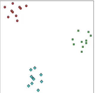
A human being has little difficulty finding groups of data objects, especially when a small number of data objects is plotted in two dimensions (two features). Figure 1.1 displays such a two dimensional plot of thirty data objects. Three clusters are shown, helpfully displayed as red circles, green rectangles, and blue diamonds. People will have little difficulty detecting the three clusters, even if the data objects are displayed in the same shape and color.
Figure 1.1: A Simple Clustering Scenario
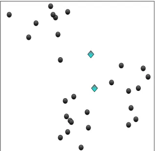
Figure 1.2 displays a slightly different two dimensional plot. Most would also decide there are three clusters in this plot. There would be ambiguity, however, as to which clusters the two blue diamond data objects belong.
One assumes intuitively that a data object can only belong to one cluster. The existence of the blue-colored data objects challenges this intuition. Can a data object be in more than one cluster simultaneously? Can a data object be assigned to no cluster at all?
The answer to both questions is yes. A clustering algorithm that assigns data objects to a single cluster is called ahard clustering algorithm. The most basic, hard clustering algorithms are discussed in Section 2.1. A fuzzy clustering algorithm allows a data object to have simultaneous
Figure 1.2: A Fuzzy Clustering Scenario
membership in multiple clusters. Fuzzy set theory and fuzzy clustering algorithms are discussed in Section 2.2. A clustering algorithm that does not necessarily assign every data object to a cluster is described in Section 2.1.3.
Fuzzy clustering algorithms have some advantages over hard clustering algorithms. The principle advantages are that a data object can belong to multiple clusters and the degree to which it belongs to these clusters is calculable. This provides more options to the data analyst. One application is image processing, where the boundary between two regions can be vague. Another possible application is clustering a Geographic Information Systems (GIS) dataset of land parcels. If the underlying groups and structure pertain to land usage, one may discover parcels used for multiple purposes.
1.2 Handling Big Data
Unfortunately, cluster analysis is not an exercise as simple as viewing Figure 1.1 or 1.2. Datasets typically have a large number of data objects and three or more dimensions, making plotting of objects and visual assignment of them to clusters infeasible. Therefore, non-trivial datasets are clustered using computer-based algorithms.
Electronic datasets have been growing in size for decades. Huber discussed in 1994 a clas-sification system for dataset sizes, which ended with the term “monster” to describe a dataset having 1012 data objects [15]. Such a system proved unsuitable for Havens, who extends Huber’s classification with the Very Large (VL) dataset, which has>1012 data objects [16].
The larger volumes of data available today are typically called “Big Data” [17]. The definitions for Big Data are generally subjective.
Madden offers such a subjective definition for Big Data. He describes Big Data as data “too big, too fast, or too hard for existing tools to process” [18]. So the conception of Big Data is relative to one’s power to deal with it. Jacobs defines Big Data in this context by its effects, namely as “data whose size forces us to look beyond the tried and true methods that are prevalent at the time” [19]. Ratner states that Big Data is in the mind of the data analyst; how much data is needed for it to be “Big” is subjective. He then goes on to describe necessary qualities of data to be considered “Big.” One quality comes from the field of classical statistics, where the sample size is so large that the “asymptotic properties of the method kick in for valid results” [20].
In summary, a Big Data dataset is cumbersome because of its size, but valuable because of the information it potentially contains.
Clustering algorithms are only one of many analytic tools that can be applied to Big Data. The runtime for a typical clustering algorithm will scale linearly to quadratically, with respect to the number of data objects. The larger the dataset, the longer the algorithm will take to produce a partition. Processing the entire dataset with typical clustering algorithms can be infeasible for real-world applications, taking more time than a required decision about the data allows.
Techniques are therefore needed to accelerate the clustering algorithms. A related challenge is to preserve the quality of the clustering algorithm’s results while accelerating its operation simul-taneously. The quality should be equivalent to clustering all the data with a classical algorithm. These areas are the subject of this dissertation.
I used large datasets for experimentation, but not truly “Big Data.” An implied task is to report the differences in runtime and quality of the accelerated clustering algorithms when compared to basic algorithms. If the datasets were so large as to be Big Data, the runtime of the basic algorithms
on the full datasets would preclude receiving results in a timely fashion. Thus, I infer from the runtime complexity of the algorithms and the results of smaller scale experiments, the expected performance on Big Data.
1.3 Contributions
I investigated the key algorithm design principles that accelerate fuzzy clustering algorithms while preserving quality. Quality is defined as closely approximating well known fuzzy clustering algorithms. My investigation identified four main ideas to apply to the development of accelerated fuzzy clustering algorithms on Big Data:
1. Use of a statistically significant sample of the dataset reduces runtime while preserving quality. 2. An algorithm designed to cluster the data incrementally can produce a high-quality result when stopped before all data has been processed. This is especially true when the data is presented in random order.
3. The use of representative objects, either weighted or un-weighted, can overcome difficulties of scale, if properly utilized.
4. For a particular class of clustering algorithms, providing a “starting point” close to the optimal solution reduces runtime and can improve quality.
None of these ideas are original. All are sound, previously-used tools for the construction of accelerated clustering algorithms. The contributions made in this dissertation are unique, fully developed, implemented strategies to employ these ideas to accelerate fuzzy clustering. The specific contributions of this dissertation are as follows:
• Identification of a statistical method never before used with accelerated fuzzy clustering al-gorithms. This method estimates the minimum sample size required to represent each cluster proportionally. I modified the statistical formula to make it compatible with clustering algo-rithms.
• Creation of an early stopping criterion for incremental or “single pass” algorithms. This criterion determines the point at which processing additional data will have little added benefit. This allows the clustering algorithm to terminate early, providing a greater speedup with little loss in quality.
• Different methods of combining representative objects were explored using fuzzy clustering al-gorithms which produce partitions by minimizing an objective function. I discovered that the best method used information from the intermediate results to improve quality and speedup.
• I developed a new method to combine representative objects in the context of density-based fuzzy clustering algorithms.
• I created five original algorithms that apply these contributions and the four main ideas listed above.
1.4 Organization
In Chapter 2, I provide detailed background on relevant clustering algorithms, accelerated variants, and metrics used to assess performance. In Chapter 3, I describe the data used for experiments.
In Chapter 4, a series of exploratory experiments are documented. Observations made from the experimental results were condensed into the four main ideas identified above.
In Chapters 5, 6, and 7 these ideas are developed into the specific contributions made to the field of Computer Science. To demonstrate the value of these contributions, five original algorithms we created implemented these contributions. Experimentation and discussion are included.
Chapter 2: Background
“It’s d´ej`a vu all over again.” - Lawrence “Yogi” Berra [2]
2.1 Basic Clustering Algorithms
Many clustering algorithms have been developed over the last five decades [5]. Only a relatively small number of algorithms out of the number available could be chosen to be the focus of my dissertation. One can categorize the choices by considering different types of clustering algorithms. A taxonomy of clustering algorithms was described by Jain [3]. One distinction made in his tax-onomy is whether the clustering algorithm is hierarchical or partitional. A hierarchical algorithm produces a nested grouping of partitions; at each level of the hierarchy there is a different number of clusters. A partitional algorithm produces a single partition with a fixed number of clusters.1
One can distinguish partitional algorithms as to whether the basis for partition is minimizing an objective function or density-based [3] [5]. In a density-based algorithm, clusters are defined as regions of high density, separated by regions of low density [24, 5].
Three of the most basic clustering algorithms of these types are described below. Each basic algorithm selected is the original or best-known representative of its type: hierarchical (Single Linkage), objective function minimizing (Hard c-means), and density-based (DBSCAN).
2.1.1 Single Linkage (SL)
Of the three basic algorithms, Single Linkage is the oldest. The first work that suggests Single Linkage, initially published in French and Polish in 1951, was rediscovered in 1957 and published in English [25].
1
Some of the material in this chapter has been previously published by me [21] [22] [23], and is re-used under terms of the copyright c 2010, 2012 and 2013 IEEE.
Single Linkage, also referred to as “Single Link” or “Nearest Neighbor,” is a hierarchical, ag-glomerative clustering algorithm. It employs a dissimilarity coefficient, ρ(xi, xj), that defines the degree to which two data objects in dataset X are dissimilar [26]. For numeric data, ρ(xi, xj) is often a distance metric, such as the Euclidean distance.
At the beginning of the algorithm, each data object in the dataset (xi ∈ X) is considered to be its own cluster. The algorithm merges into a single cluster the two clusters (which initially are data objects) that are least dissimilar. Single Linkage repeats the merging of the least dissimilar clusters until all ndata objects inX have been assigned to a single cluster.
A formal description, adapted from [27], is presented as Algorithm 1. For efficiency, implemen-tations of the algorithm usually store the dissimilarities in a dissimilarity matrix.
The algorithm returns a list of merges,M. The decision to merge two clusters is based on the dissimilarity coefficient. Thus, given a dataset, a dissimilarity coefficient, and rules for tie-breaking, Single Linkage is deterministic in that it will always return the same list of merges [27].
Single Linkage begins withn clusters. With each merge, the number of clusters is reduced by 1. If the cluster assignments prior to each merge are listed, a numeric hierarchy of heightn−1 is created. A dendrogram is the most common way to display a hierarchy.
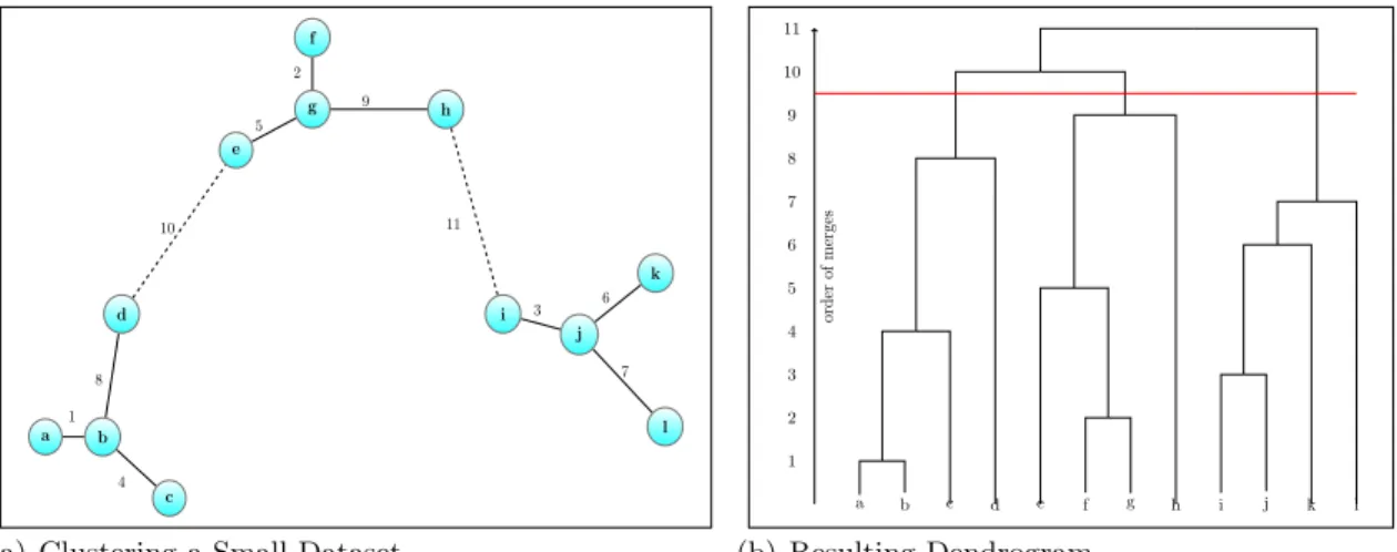
This process is shown in Figure 2.1. Figure 2.1(a) shows a simple dataset consisting of 12 data objects. Merges are indicated by line segments connecting two data objects. Each line segment is annotated with a number to show the order of the merges. Note that data objects a and b are connected with a line segment annotated with a ‘1’. This is the first merge. Likewise, the ‘2’ between objectsf and g indicates the second merge. Alln−1 merges are shown in Figure 2.1(a). Figure 2.1(b) shows the dendrogram that displays the hierarchical structure created by Single Linkage. The y axis shows the order of the merges connecting data objects. The number assigned to the merge is also called a splitting level [25].
A human would typically consider the dataset shown in Figure 2.1(a) as having three clusters. If Single Linkage were halted after splitting level 9, the merges labeled ‘10’ and ‘11’ would not be made and three clusters would remain. The red line in Figure 2.1(b) shows the effect on the dendrogram.
Algorithm 1:Single Linkage 1: Input: X,ρ(xi, xj)
2: for i= 1 to ndo
3: L[i] =i(each initial cluster is labeled with the index of its data object) 4: forj= 1 to ido
5: D(xi, xj) =D(xj, xi) =ρ(xi, xj)
6: end for 7: end for
8: for k= 1 to n−1 do
9: (a, b) =argmin(a,b):D(a,b)6=−1D(a, b)
10: M.append(a, b)
11: D(a, b) =D(b, a) =−1 12: forj= 1 to n do 13: if L[j] =b then
14: L[b] =a(clusterbis now part of cluster a) 15: end if 16: D(a, xj) =D(b, xj) =min(D(a, xj), D(b, xj)) 17: end for 18: end for 19: return M where:
X is a dataset consisting of ndata objects.
ρ(xi, xj) is the dissimilarity coefficient.
xi is the ith data object in X.
D is the dissimilarity matrix andD(xi, xj) is the dissimilarity between xi andxj.
D(a, b) =−1 indicates objects aand b are in the same cluster.
L is an array holding the current set of cluster labels.
M is an ordered list holding the pairs of merges.
If the dataset is small, examining a dendrogram visually can reveal the number of clusters. When the dataset is larger, some method is needed in order to split the hierarchy represented by the dendrogram. Three of the many methods for splitting the dendrogram are described by Manning [27].
The first method splits the dendrogram at a user-defined value of dissimilarity. Note that the dissimilarity between objects increases monotonically as they are merged by Algorithm 1. Thus, if a particular value of dissimilarity were exceeded, all subsequent merges would be of this value or greater. The second method calculates the difference between the successive dissimilarities during
a b c d e f g h i j k l 1 2 3 4 5 6 7 8 9 10 11
(a) Clustering a Small Dataset
a b c d e f g h i j k l order of merges 1 2 3 4 5 6 7 8 9 10 11 (b) Resulting Dendrogram
Figure 2.1: Clustering with Single Linkage
Numbers indicate the order of the merges. Dotted links are merges that would not be made if three clusters are desired.
the merge process. The splitting level at which this difference is greatest is used. The third method splits the dendrogram in order to produce a predefined number of clusters.
A criticism of the Single Linkage algorithm is that clearly distinct clusters (from an observer’s perspective) can be prematurely merged together due to a single pair of nearby objects or a noisy dataset. This phenomenon is called “chaining” [28] [25]. It has been pointed out that chaining is not a flaw, but rather a feature of hierarchical clustering which may be desirable given a particular dataset and application [26].
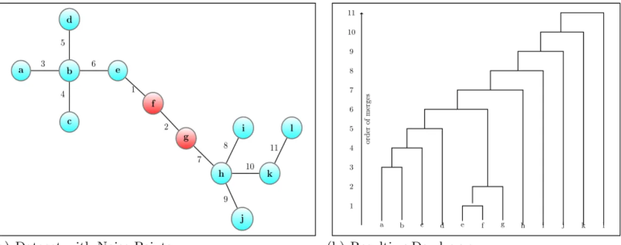
Figure 2.2 shows the effect of ill-placed noise objects on a simple dataset. Data objects ‘f’ and ‘g’ are noise and unfortunately placed between two natural clusters represented by data objects a-e and h-l respectively. Figure 2.2(a) shows the order of merges. The first two merges have a dissimilarity ofδ; all subsequent merges have a dissimilarity ofδ+. Contrast the resulting dendrogram (Figure 2.2(b)) with the previous example (Figure 2.1(b)). In this dendrogram, the structure of the data is more difficult to discern.
There are many variants of Single Linkage, some of which are designed to avoid the chaining effect [27] [28] [26]. Of these, the best known are Complete Linkage and Average Linkage. Complete Linkage merges clusters based on the most dissimilar data objects in each cluster, as opposed to the
a b c d e f g h i j k l 1 2 3 4 5 6 7 8 9 10 11
(a) Dataset with Noise Points
a b c d e f g h i j k l 1 2 3 4 5 6 7 8 9 10 11 order of merges (b) Resulting Dendrogram
Figure 2.2: Single Linkage Chaining
Numbers indicate the order of the merges. The red-colored data objects are noise.
least dissimilar [27]. Average Linkage merges clusters based on the average dissimilarity between data objects in each cluster [28].
Algorithms in the Single Linkage family have many scientific applications, including bioinfor-matics [29] and document clustering [27].
2.1.1.1 Runtime Complexity
A literal implementation of Single Linkage has a time complexity of O(n3), where n is the number of data objects [25] [27]. In line 9 of Algorithm 1, the dissimilarity matrix D is searched exhaustively for the pair of clusters that have the minimum dissimilarity. D has a size of O(n2), and line 9 is executed O(n) times, resulting in a runtime complexity ofO(n3).
Sibson developed an improved implementation of Single Linkage with a runtime complexity of
O(n2) [25]. A similar implementation appears in [27]. Improved implementations exist for the variants of Single Linkage with runtime complexities of O(n2log(n)) [27]; the need to recalculate the dissimilarities at each merge stymies the development of anO(n2) algorithm.
2.1.2 Hard c-means (HCM)
The hard c-means (HCM) algorithm, attributed to MacQueen [30], was independently discov-ered multiple times [31] [28]. This algorithm, though typically called k-means clustering, is referred
to here as hard c-means in order to conform with the conventions of the fuzzy clustering literature [32].
HCM is a distance-based, partitioning algorithm [3]. It clusters a dataset in which each data object consists of a vector of sfeatures. The HCM algorithm seeks to reduce the sum of squared error, represented by the square of the Euclidean distance between each data object and its closest respective cluster center [3] [28] [33]. The value of the sum of the squared error for a partition is:
J = c X j=1 n X i,xi∈cj ||xi−cj||2 (2.1) where:
J is the sum of the squared error.
X is a dataset where n=|X|, and xi is the ith data object.
C is the set of cluster centers wherec=|C|, and cj is the jth cluster center.
The partition produced by HCM is defined by:
Xj ={xi :||xi−cj||2 ≤ ||xi−ck||2 ,1≤i≤n, 1≤k≤c} (2.2) where:
n,xi, and cj are defined as above, and
Xj is the subset of data objects from X belonging to thejth cluster.
In cases where a data object is equidistant from two or more cluster centers, the object must be arbitrarily assigned to one of the clusters. The simplest solution to implement is to assign the object to the cluster center with the lowest index.
The cluster center, cj, is represented by ans-dimensional vector. Given the entire set of data objectsXj ⊂X belonging to cluster j, the cluster center can be calculated by:
cj = 1 |Xj| X xi∈Xj xi (2.3)
Finding the set of cluster centers that minimizes J is an NP-hard problem [34]. The HCM algorithm’s strategy for minimizing Equation 2.1, is to alternate between Equations (2.2) and (2.3). An algorithm that uses a pair of equations in this way is said to use Alternating Optimization (AO) [35]. An initial set of cluster centers, C, is required for Equation 2.2. A termination criterion is also required for HCM.
While there are several initialization strategies [3], the most common strategy is to randomly select a set of c data objects to provide the initial positions of the cluster centers [33]. HCM terminates when Equation (2.2) results in no data object changing its currently assigned cluster. Alternatively, HCM can be implemented to terminate if the difference between successive values forJ does not exceed a user-defined value. A more formal description is as follows [3] [33]:
Algorithm 2:Hard c-means 1: Input: X,c
2: Choose c data objects from X to provide initial cluster centers for C
3: Assign each data object to the nearest cluster center using Equation 2.2 4: while At least one cluster assignment changes for xi ∈X do
5: Update all cj ∈C using Equation 2.3
6: Assign each data object to the nearest cluster center using Equation 2.2 7: end while
8: return C
One must consider some limitations when using HCM to cluster data. The first is that the HCM algorithm requires an initial set of cluster centers, which implies that the number of clusters is known [3]. The second is that the HCM algorithm is non-deterministic if this initial set of clusters is chosen randomly [27]. The final set of cluster centers returned by HCM is highly dependent on the initial set of clusters provided [3]. The third limitation is that all clusters will be hyperspherically shaped, since each data object is assigned to the nearest cluster center.
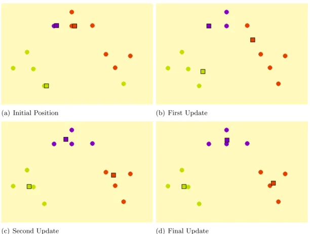
Figure 2.3 shows how HCM clusters a simple dataset. In the subfigures, circles represent the data objects (X), squares represent the cluster centers (C), and data objects are assigned to cluster
assignments. The squares representing the cluster centers are slightly offset to show the data objects beneath. Subfigures 2.3(b), 2.3(c), and 2.3(d) show three successive iterations of the cluster center positions and cluster assignments on line 6 of Algorithm 2. In the final subfigure, the data objects will not change their currently assigned cluster and HCM will terminate.
The series of images demonstrating k-means were produced from an interactive online resource [36].
(a) Initial Position (b) First Update
(c) Second Update (d) Final Update
Figure 2.3: Clustering with Hard c-means
2.1.2.1 Runtime Complexity
The HCM algorithm has a time complexity ofO(nisc), where nis the number of data objects,
i the number of iterations, s the number of features, and c the number of clusters [33]. This can be verified by examining Algorithm 2 and Equations 2.2 and 2.3.
Equation 2.2 is calculated on line 3 of Algorithm 2. This equation requires a comparison of the squared distance of every data object to every cluster. The distance calculation requiresO(s) time, and the distance is calculatedO(nc) times, for an overall time complexity ofO(nsc).
Equation 2.3 is calculated on line 5 of Algorithm 2. This equation finds the average position of the data objects assigned to each respective cluster. This can be implemented in O(ns) time. On line 6, Equation 2.2 is calculated again.
Lines 5 and 6 of Algorithm 2 are executed once per iteration, i, until HCM terminates. The total time complexity (T) is therefore:
T =O(nsc) +i×(O(ns) +O(nsc)) =O(nsc) +O(nis) +O(nisc) =O(nisc)
2.1.3 Density Based Spatial Clustering of Applications with Noise (DBSCAN) DBSCAN is a density-based clustering algorithm, first published in 1996 [24]. Its similarity to the earlier Jarvis-Patrick algorithm [37] and Parzen window density estimation [38] was noted by Jain [5].
Conceptually, DBSCAN works as follows. An s-dimension space is defined by the features of the data objects in a dataset (X). DBSCAN partitions this space into two types of regions, dense regions considered part of a cluster and sparse regions not considered part of a cluster. Data objects in the former region are assigned to a cluster, whereas any data objects in the latter region are considered to be noise. Data objects in a contiguous region of “dense” space are assigned to the same cluster.
DBSCAN then overcomes the limitations of the distance-based HCM algorithm described in Section 2.1.2, namely that the: (1) number of clusters must be known in advance, (2) clusters are hyperspherical, and (3) all data objects must belong to a cluster [21].
The local density at each data object is assessed using two parameters,ε(distance) andM inP ts
(a lower bound on the minimum number of points, i.e., data objects). A single data object is considered a “core point” if it is located within ε distance of at least M inP ts data objects. All data objects withinεdistance of a core point are considered members of its cluster [21].
Clusters are created from multiple core points located withinεdistance from each other. Other non-core data objects within ε distance of a core point are assigned to that core point’s cluster. These non-core data objects are called “border points.” As a result, large, irregularly shaped clusters can be found. As mentioned above, data objects not assigned to a cluster are considered noise [21].
The original presentation of DBSCAN, presented below as Algorithm 3, formally defines a number of terms to clarify how the algorithm works [24]:
1. εNeighborhood (Nε(xi)): The set of data objects within distanceεof data object xi.
2. Core Point: A data object,xi, where|Nε(xi)| ≥M inP ts.
3. Border Point: A data object, xi, where |Nε(xi)| < M inP ts, xi ∈ Nε(xj) and xj is a core point.
4. Directly density-reachable: Data object, xi, is directly density-reachable from xj if xi ∈
Nε(xj) and xj is a core point.
5. Density-reachable: Data object,xi, is density-reachable fromxj if there is a chain of directly density-reachable core points between them.
6. Density-connected: Two data objects, xi and xj, are connected if both are density-reachable to some data objectxk.
When a core point,xi, not assigned to a cluster is identified on line 12, the algorithm discovers all data objects directly density-reachable from xi. Subsequently, a recursive call of the Function ExpandCluster on line 17 allows DBSCAN to find all objects density-reachable from the original core point. Line 16 ensures the same cluster assignments both for border points and core points.
Algorithm 3:DBSCAN 1: Input: X,ε,M inP ts
2: Assign each data object in X a cluster ID number = 0 (xi.id= 0)
3: ClustId= 1 4: for i= 1 to ndo 5: if xi.id= 0 then 6: ExpandCluster(xi) 7: end if 8: end for 9: Function ExpandCluster(xi)
10: if |Nε(xi)|< M inP tsthen {xi is not a core point}
11: return
12: else {xi is a core point}
13: xi.id=ClustId
14: C=Nε(xi)
15: for allxj ∈C do{xj is a member ofxi’s cluster}
16: xj.id=ClustId 17: ExpandCluster(xj) 18: end for 19: ClustId=ClustId+ 1 20: return 21: end if where:
X is a dataset consisting of ndata objects.
εis a distance.
M inP ts is an integer.
xi is the ith data object in X. Cis a set of data objects.
A ClusterID = 0 signifies the data object is NOISE.
DBSCAN requires two parameters, ε and M inP ts, which define the threshold density for a cluster. These values can be set empirically. Ester provides a method to set them that works well in low dimensions [24].
2.1.3.1 Runtime Complexity
A naive implementation of DBSCAN has a runtime complexity ofO(n2). Discovery of all data objects in Nε(xi) requires calculating the distance between xi and ∀xj ∈ X. This step, which
occurs on line 10 of Algorithm 3, has a time complexity O(n) and is executed O(n) times (line 4 of Algorithm 3).
If the dataset were sorted into a structure such as an R* tree [39], the discovery of all data objects in Nε(xi) would have an average runtime complexity of O(log(n)). If this precondition is met, DBSCAN has a runtime complexity ofO(n log(n))
2.2 Algorithms Based on Fuzzy Sets
2.2.1 Fuzzy Sets and Logic
The clustering algorithms discussed in Section 2.1 are based on classical set theory. These algorithms produce a crisp partition that assigned data objects to a single cluster. A crisp partition can be expressed as a binary membership matrix, U, where uik ∈ {0,1} refers to the membership value of thekth data object, xk, in theith cluster.
In contrast, fuzzy set theory allows an object to have varying grades of membership in a set [40]. When fuzzy sets are used in a clustering algorithm, a data object can have a grade of membership in multiple clusters [21]. A fuzzy clustering algorithm produces a fuzzy partition which can also be expressed by a membership matrix, U. The grade of membership of a data objectk in clusteriis uik. This is subject to the following constraints [41] [22]:
uik ∈[0,1],1≤i≤c,1≤k≤n (2.4) c X i=1 uik= 1,1≤k≤n (2.5) n X k=1 uik >0,1≤i≤c (2.6)
wheren is the number of data objects andcis the number of clusters.
Fuzzy approaches have been successfully integrated in many clustering algorithms [32] [42] [43] [44] [45]. Three such applications are discussed in this section.
2.2.2 Fuzzy c-means (FCM)
The Fuzzy c-means (FCM) algorithm, developed by Bezdek [41], is based on earlier work by Ruspini and Dunn [28] [5]. As the name suggests, it is a fuzzy variant of HCM.
FCM produces a set of c cluster centers by approximately minimizing the objective function that calculates the within-group sum of squared distances from each data object to each cluster center. FCM alternates between calculating optimal cluster centers, given the membership values of each data object, and calculating membership values, given the cluster centers [22]. If data objects are defined as feature vectors, xk in Rs, the objective function (Jm) is expressed as [23]:
Jm(U, V) = c X i=1 n X k=1 umikDik(xk, vi) (2.7)
The functions for determining optimal membership values and optimal cluster centers are derived from Equation 2.7 using Lagrange multipliers [41]:
uik = Dik(xk, vi) 1 1−m Pc j=1Djk(xk, vj) 1 1−m (2.8) vi = Pn j=1(uij)mxj Pn j=1(uij)m (2.9) where:
X is a dataset where n=|X|, and xi is the ith data object.
m >1 controls how fuzzy the clusters are.
cis the number of clusters.
U is the membership matrix; uik refers to the membership value of the kth data element (xk) for theith cluster.
V is the set of cluster centers; vi is the ith cluster center.
Dik(xk, vi) is the squared distance between thekthdata object and ith cluster center; any inner product induced distance metric can be used (e.g. Euclidean).
There are implementation options. TheU orV matrices may be initialized with any valid set of values. Typically, the uik are initialized with a set of values adhering to (2.4) to (2.6) or each vi is set to equal the position of a randomly selected data object in X. The FCM algorithm terminates when the difference between successive membership matrices or sets of cluster centers does not exceed a given parameter [22]. Algorithm 4 describes the implementation used in this research.
Algorithm 4:Fuzzy c-means 1: Input: X,c,m,
2: Choose c data objects from X to provide initial positions for V
3: Assign initial cluster membership values using Equation 2.8.
4: maxChange= 1 +
5: while maxChange > do 6: Uprev=U
7: Update all vi∈V using Equation 2.9.
8: Reassign cluster memberships to each data object using Equation 2.8. 9: maxChange=calcM axChange(U, Uprev)
10: end while 11: return U, V
The functioncalcM axChange(U, Uprev) returns the maximum difference in cluster membership (uik) across two iterations.
2.2.2.1 Runtime Complexity
A literal implementation of the FCM algorithm has an expected runtime complexity ofO(nisc2)
[46], where nis the number of data objects,c the number of clusters,sthe dimension of the data, and i the number of iterations. An optimization proposed by Kolen and Hutcheson [47] reduces the runtime toO(nisc). The remainder of this work uses Kolen’s optimization. For details, see [47] and Section A.2.3.
2.2.3 Fuzzy c-medoids (FCMdd)
The HCM and FCM algorithms assume that the data objects are represented by numeric feature vectors. Both algorithms produce cluster centers located in Rs, the feature space of the dataset.
Not all datasets, however, consist of data objects represented by feature vectors. Relational data objects, as opposed to numeric (i.e., object) data, do not have a representation in Rs [48]. For relational data, a measure for similarity or dissimilarity between a pair of data objects can be defined. A dissimilarity coefficient,ρ(xi, xj), as described in Section 2.1.1, is typically used.
Single Linkage and DBSCAN do not produce cluster centers inRs. They therefore can produce clusters from either numeric or relational data. Single Linkage requires no modification to do so. DBSCAN requires that “distance” be replaced with ρ and that the parameter be appropriately set.
HCM and FCM require modification to accept relational data. Conceptually, HCM and FCM both seek to minimize an objective function based on the total squared error of a partition of the data. When using relational data, minimization of such an objective function is still possible.
Hathaway modified Equation 2.7 to accommodate relational data [48]. This modification sub-stituted a mean cluster membership vector for cluster centers. Versions include Relational Hard c-means (RHCM), Relational Fuzzy c-means (RFCM), and Non-Euclidean RFCM (NERF) [48] [49].
One can also select representative data objects from the dataset as cluster centers. When discussing clustering algorithms, such representative objects are referred to as medoids. In the field of Operations Research, variations of this problem are known as the facility location problem and k-median problem [50] [28].
Crisp set versions of a “Hard c-medoid” algorithm include Partitioning Around Medoids (PAM), and Clustering Large Applications (CLARA) [51] [28]. Its fuzzy set version is Fuzzy c-medoids (FCMdd) [44]. Krishnapuram originally developed the FCMdd algorithm to cluster textual data [52] [44].
FCMdd minimizes the objective function Jm.
Jm(V, X) = n X i=1 c X j=1 umijρ(xi, vj) (2.10)
where:
X is a dataset where n=|X|, and xi is the ith data object.
m >1 is the “fuzzifier.”
cis the number of clusters.
U is the membership matrix;uij refers to the membership value of theith data element (xi) for thejth cluster.
V is the set of cluster centers; vj is thejth cluster center.
ρ(xi, vj) is the dissimilarity between theith data object and jth cluster center.
The same membership function used for FCM can be used for FCMdd if the squared distance is replaced with the dissimilarity. Although other membership functions can be used [44], I imple-mented Equation 2.11 for the work described here.
uij = ρ(xi, vj) 1 1−m Pc k=1ρ(xi, vk) 1 1−m (2.11) Like FCM, FCMdd is provided an initial set of medoids,V. Note that unlike FCM, the medoids are always data objects,xi. It then alternates between calculating the membership matrix,U (based on the values inV), and calculating new medoids,V (based on the values inU), until a termination criterion is met.
Unfortunately, no equation is provided for the optimization of the medoids. FCMdd is not a true alternating optimization algorithm, and a Lagrangian “hill-climbing” formula cannot be used as with FCM [41] [44].
Selection of the optimalcmedoids that reduce the value ofJm for the current values inU would require testing nc
combinations. Clearly, this is intractable, so a heuristic proposed by Fu [53] is used. The heuristic keeps all but one vj ∈ V fixed, and it evaluates the remaining n−c data objects in xi ∈X. If there are any xi, if substituted for vj in Equation 2.10, that would result in a lower value for Jm, the xi that would minimize Jm replaces vj in V. Each vj ∈ V is considered per iteration.
FCMdd’s initialization and termination criterion remain to be discussed. Initialization of FCMdd requires the selection of c medoids to populate V. The most obvious technique is to selectcdata objects randomly. Empirically, Krishnapuram noted that FCMdd often would become stuck in local extrema if this technique was used [44].
An alternative technique is to randomly select a single data object,xi, to insert into V. Then, the data object, xj ∈ X, with the greatest dissimilarity from xi should be selected and placed into V. For the remaining c−2 medoids, each successive data object, xk ∈X, with the greatest sum of dissimilarity to all objects currently inV will be selected. This technique, described in [52] as “Initialization III,” experimentally produces higher-quality partitions than those produced by random selection. Initialization III was used in research.
Similarly to HCM, the FCMdd algorithm terminates whenV remains unchanged between up-dates toU. FCMdd also terminates if it reaches a maximum number of iterations (M AX IT ER). In the implementation for research,M AX IT ERwas hard-coded to equal 100. It was noted in [54] that the algorithm can get stuck in a cycle where the medoids inV alternate between two assign-ments until M AX IT ER is reached. This condition was tested for also. If V, in iteration i, had the same assignments asV, in iterationi+ 2, the algorithm terminated. A single test is sufficient, because the update process is deterministic for a given dataset and starting set of medoids.
The formal description of FCMdd as listed in Algorithm 5 is slightly modified from its original publication [44].
2.2.3.1 Runtime Complexity
Krishnapuram reported the runtime complexity of FCMdd as O(n2) [52]. If the number of iterations, i, and the number of clusters,c, are considered, the runtime complexity will be higher. An in-depth analysis of runtime complexity follows. One assumption made in the analysis is that the dissimilarity between two data objects can be calculated in constant time.
On line 2 of Algorithm 5, the initial set of medoids is selected. This initialization technique has a runtime complexity ofO(nc2) [52]. Thewhilestatement on line 5 is executeditimes. Within the whilestatement, the membership matrix is updated on line 7. This step has a runtime complexity
Algorithm 5:Fuzzy c-medoids 1: Input: X,c,m
2: Select cdata objects from X to provide an initial set of medoidsV. 3: Set Vold=N U LL
4: Set IT ER= 0
5: while (Vold 6= V and IT ER < M AX IT ER) do
6: Vold=V
7: Update membership matrixU using Equation 2.11 8: forj= 1 to c do 9: p= argmin(1≤k≤n) Pn i=1umijρ(xk, xi) 10: vj =xp 11: end for 12: IT ER=IT ER+ 1 13: end while 14: return C
of O(nc). Also within the while statement, on line 9, an estimate is calculated of the impact of changing vi. This step has a runtime complexity ofO(n2), is within the for loop on line 8, and is executed ctimes. The total runtime complexity (T) is therefore:
T =O(nc2) +i×(O(nc) +c×O(n2)) =O(nc2) +O(nci) +O(n2ci) =O(n2ci)
2.2.4 Fuzzy Neighborhood DBSCAN (FN-DBSCAN)
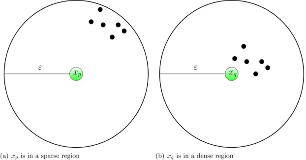
Nasibov and Ulutagay modified the DBSCAN algorithm to integrate fuzzy set theory [45]. Fuzzy Neighborhood Density-Based Spatial Clustering of Applications with Noise (FN-DBSCAN) employs a fuzzy neighborhood function rather than a crisp set definition to assess density [55]. FN-DBSCAN repairs one of FN-DBSCAN’s flaws [21]. Since FN-DBSCAN uses a crisp definition for density, a data object, xp, at nearly εdistance from a group of data objects, is assigned the same density as a data object,xq, in close proximity to a similar group of data objects (Figure 2.4 ).
x
pε
(a)xpis in a sparse region
x
qε
(b) xq is in a dense region
Figure 2.4: Data Objects xp and xq Have Same Density in DBSCAN, but Have Different Densities in FN-DBSCAN
FN-DBSCAN corrects the density calculation by using a fuzzy membership function, where the density at a data object is the sum of the values of the fuzzy membership functions of all data objects within distance ε. Otherwise, the algorithm is identical to DBSCAN. Many fuzzy neighborhood membership functions have been developed; Nasibov and Ulutagay discussed the use of linear, trapezoidal, and exponential fuzzy neighborhood functions [56] [45].
The linear fuzzy neighborhood function, the most straightforward, is defined as [45]:
µ(xi, xj) = 1−(ρ(xi, xj)/ε), ifρ(xi, xj)≤ε 0, otherwise (2.12)
whereρ(xi, xj) is the distance between data objectsxi and xj.
Figure 2.5 shows how the value of the fuzzy neighborhood function varies with distance. The figure assumes that the data is scaled so that the maximum dissimilarity is equal to one.
A choice of fuzzy neighborhood function must be supplied to FN-DBSCAN as a parameter. Because the focus of my dissertation is to reduce the runtime of fuzzy clustering algorithms, the choice of the fuzzy neighborhood function is not an important factor as long as the choice is the same
0 ε 1 0 0.2 0.4 0.6 0.8 1 ρ(xi, xj) µ ( xi , xj )
Figure 2.5: Linear Neighborhood Function Used in FN-DBSCAN
for all experiments. Therefore, the simplest fuzzy neighborhood function, the linear neighborhood function, was used.
Like DBSCAN, FN-DBSCAN requires two additional parameters: distance, ε, and minimum cardinality, M inCard. The term “minimum cardinality,” used instead of “minimum number of points,” accurately reflects how FN-DBSCAN uses the sum of the fuzzy neighborhood function values for each data object to calculate the density. If, for a data object, the fuzzy set cardinality,
F SCard, is greater thanM inCard, that data object is a core point [45] [55].
F SCard(xi) = n
X
j=1
µ(xi, xj) (2.13)
Except for this change, the FN-DBSCAN algorithm is identical to DBSCAN [21]. The runtime complexity is also identical.
2.3 Accelerated Clustering Algorithms
2.3.1 Significant Work Related to Acceleration
The focus of my dissertation is to reduce the runtime of fuzzy clustering algorithms while keeping quality loss to a minimum. As clustering algorithm research has has intense focus for five decades, there has been and continues to be much interest in accelerating clustering algorithms. This section describes significant work relevant to the methods used and experiments described in this dissertation. Accelerated algorithms, used for experiments in the research or related to this work, are described in the sections below.
A literal implementation of the FCM algorithm, as described in Section 2.2.2.1, has an expected runtime complexity of O(nisc2), wheren is the number of data objects,c the number of clusters,
s the number the data features, and i the number of iterations. As previously mentioned, it is possible to reduce the runtime toO(nisc) with the optimization proposed by Kolen and Hutcheson [47].
Given a dataset withcnatural clusters, an FCM variant can be accelerated further by reducing
n,s, ori. There are techniques for reducing the number of features,s, but many of these techniques preprocess the data rather than being integrated into the algorithm itself [57] [58]. An alternative technique, subspace clustering, looks for clusters using a subset of the available features [59] [60]. Each cluster found can use a different subset of the available features. This line of research, however, was not pursued. My dissertation focused on techniques that reduce the amount of data used, n, and the number of iterations, i.
Algorithms such as FCM, designed to minimize an objective function value, have shorter run-times if their initial cluster centers are close to the final solution. The shorter runtime is due to a reduction in iterations before termination. Bradley and Fayyad [61] investigated the effects of an improved starting position for HCM. A better start position reduced the runtime, but their study was focused on quality, not speed.
Processing a small data sample to obtain an improved initial starting point for FCM has been investigated. Cheng describes an iterative process to develop a “good” starting point [62]. This
method, Multistage Random Sampling FCM (mrFCM), consists of two parts. The first part pro-gressively samples the dataset, improving the starting clusters until a termination criterion is met. Then mrFCM uses these starting clusters to initialize FCM on the full dataset.
Similarly, Altman uses FCM to obtain a set of cluster centers from a small sample of data objects. These cluster centers are used to initialize the membership matrix, U, before clustering the full dataset with FCM [63].
In Partition Simplification FCM (psFCM), Hung and Yang [64] partition the data using a k-d tree to obtain a simplified dataset, which in turn is used as a subsample to estimate the position of the cluster centers. The resulting estimate is used to initialize FCM on the full dataset.
The Single Pass FCM (SPFCM) algorithm, discussed in Section 2.3.2, incrementally clusters the data and passes on the cluster centers from each increment as an initialization for the next [46]. Online FCM (OFCM), discussed in Section 2.3.3, follows a similar strategy [65].
Provost presented an overview of the progressive sampling technique in the context of induc-tion (a.k.a. classificainduc-tion) algorithms [66]. Progressive sampling uses an initial subsample to form a classifier, which is tested on labeled data. The subsample progressively increases in size arith-metically or geometrically, creating a new classifier each time it grows. When the accuracy of the classifier ceases to improve significantly when compared to the previous sample, the addition of data is terminated.
Progressive sampling techniques have been applied to clustering problems. These techniques accelerate a clustering algorithm by reducing the number of data objects, n, that are clustered.
Domingos and Hulten [67] used Hoeffding bounds in a progressive sampling technique both to estimate the initial sample size and to estimate the sufficiency of the sample size at any point in the progression. The technique, developed for HCM, assumes that each data object has membership in only one cluster. It calculates the worst-case bounds, and the sample sizes are typically large.
Pal and Bezdek [68] and Wang et al. [69] used progressive sampling to select a subsample representative of the dataset. They used a divergence test to assess whether the subsample matched the distribution of the dataset. If the test failed, progressively larger subsamples were taken until
the test passed. Finally a clustering algorithm was run on the chosen subsample. This technique, extensible Fast FCM (eFFCM), is discussed in detail in Section 2.3.4.
A very simple way to reduce nis to select a sample of the dataset and to apply the clustering algorithm to the sample. Havens et al. [16] use this technique in the random sampling plus extension FCM (rseFCM) algorithm, which is discussed further in Section 2.3.5
2.3.1.1 Relational Clustering
Fewer techniques exist for accelerating relational clustering algorithms.
Clustering Large Applications (CLARA) accelerates the PAM algorithm by repetitively sam-pling the dataset [28]. Each sample is clustered using PAM, and the clustering solution is extended to the entire dataset. The clustering solution with the lowest (best) objective function is returned. The sample size and number of samples taken are user-determined.
An optimization to FCMdd is Linearized Fuzzy C-Medoids (LFCMdd). This accelerated variant, as the name suggests, reduces the runtime complexity to be linear with respect the number of data objects, i.e.,O(nci). LFCMdd considers only the data objects with the highest membership values as candidates to update the current set of cluster centers [44].
Labroche directly adapted SPFCM and OFCM to use FCMdd as the base algorithm [54]. These accelerated algorithms, History Based Online Fuzzy Medoids (HOFCMD) and Online Fuzzy C-Medoids (OFCMD), are otherwise identical to SPFCM and OFCM respectively.
Bezdek (et al.) created an accelerated, relational version of eFFCM called extended non-Euclidean relational fuzzy c-means (eNERF) [70]. The eFFCM algorithm, described in detail in Section 2.3.4, depends on the existence of features from which to select a sample of the data. These features, of course, do not exist in relational data. To solve this problem, eNERF considers relations between data objects rather than features, and then selects a subset of relations that are dissimilar to each other. The eNERF algorithm otherwise uses a strategy similar to that of eFFCM.
2.3.2 Single Pass Fuzzy c-means (SPFCM)
Prodip Hore developed SPFCM as part of his dissertation research [71]. The SPFCM algorithm breaks the dataset into equally sized “partial data accesses” (PDA). A user-provided parameter, “fractional PDA” (f P DA ≤ 0.5), defines the PDA size as f P DA×n where n equals the total number of data objects. SPFCM incrementally processes the entire dataset one PDA at a time. Each PDA is processed by a weighted version of FCM, aptly named Weighted FCM (WFCM). In the WFCM algorithm, each data object, xi, has an associated weight, wi. The objective function and cluster center calculation from Section 2.2.2 are modified as follows [46] [11]:
Jmw(U, V) = c X i=1 n X k=1 umikwkDik(xk, vi) (2.14) vi= Pn j=1wj(uij)mxj Pn j=1wj(uij)m (2.15)
wherewi is a non-zero weight for a data object.
Data objects are initially given a weight of 1. After the cluster centers, vi ∈V, are calculated from the first PDA, the cluster centers are assigned weights using the following Equation [11]:
w0i = n
X
j=1
(uij)wj,1≤i≤c (2.16)
SPFCM uses weighted cluster centers as representative objects. These weighted cluster centers represent the partition information from the first PDA. Theccluster centers are added as additional data examples to the second PDA, which is then clustered by WFCM. The positions of the cluster centers calculated from the first PDA are used as the initial values forV in the second PDA. This process is repeated until all PDAs have been clustered. SPFCM returns as a final solution the set of cluster centers from the last PDA.
The SPFCM algorithm assumes that the data objects in the dataset have been randomly or-dered. Datasets with some sort of inherent order in the data, typical in images, can result in PDAs
significantly different with respect to the overall distribution. The implementation used in this research randomizes the data prior to processing.
2.3.2.1 Runtime Complexity
The runtime complexity of FCM isO(nisc) (Section 2.2.2.1). Note that the runtime complexity is linear with respect ton, the number of data objects. The SPFCM algorithm also processes the entire dataset, albeit incrementally, so a cursory analysis of the runtime complexity would also yield O(nisc).
Hore reports that SPFCM had a shorter runtime than FCM on the datasets he tested [46]. Hore identified the cause: after the first PDA had been clustered, the derived cluster centers were used to initialize V in the subsequent PDA. Initial cluster centers closer to the optimal cluster centers allow the algorithms in the HCM family to terminate with fewer iterations [61].
Reviewing complexity analysis in a similar manner as [46] [71], the following notation is used:
nis the size of the dataset.
p is the PDA value as a fraction (fPDA).
d= 1p is the number of partial data accesses required.
ij: is the number of iterations in the jth PDA.
Tj =O(pnijsc) runtime complexity for the jth PDA ˆi=pPd
j=1ij average number of iterations per PDA
T =O(Pd
j=1pnijsc) total runtime complexity for SPFCM
T =O(nˆisc) substituting ˆiinto expression forT
(2.17)
The runtime complexity of SPFCM isO(nˆisc). When SPFCM clusters a dataset it has a shorter runtime compared with FCM because typically, ˆi < i.
2.3.3 Online Fuzzy c-means (OFCM)
Prodip Hore also developed OFCM as part of his dissertation research [71]. OFCM breaks the dataset into PDAs and clusters each PDA, in the same manner as SPFCM. The OFCM algorithm
produces a set of cluster centers from each PDA and, using Equation 2.16, calculates their weights. These weighted cluster centers represent the partition information in each PDA.
The OFCM and SPFCM algorithms, though similar, have one major difference [11]. Unlike SPFCM, OFCM saves each set of weighted cluster centers, instead of adding them to the subsequent PDA. After all PDAs have been clustered, the saved sets of weighted cluster centers from each PDA are combined into one dataset. Then, WFCM clusters this combined dataset. OFCM returns as a final solution the set of cluster centers from the combined dataset.
An advantage of OFCM is that the processing of a dataset can be separated over distance or time. In these cases, the initial set of cluster centers is chosen locally by random selection. Alternatively, cluster centers from a previous PDA can be used as initial cluster centers. While the latter strategy matches the original implementation of the algorithm [65], a PDA not representative of the entire dataset will provide a poor initial set of starting clusters. OFCM does not assume that the dataset is in random order. In this dissertation, except where explicitly noted, the datasets clustered by OFCM were not randomized.
The runtime complexity analysis of OFCM is fundamentally the same as the analysis in Section 2.3.2.1.
2.3.4 Extensible Fast Fuzzy c-means (eFFCM)
The eFFCM algorithm clusters a statistically significant sample, ˆX, as opposed to the full dataset, X. Statistical significance is tested for by comparing the distribution of the sample with the distribution of X using the Chi-square (χ2) statistic or Kullback-Leibler divergence. It is formally presented as Algorithm 6.
If the initial sample fails testing, additional data is progressively added to the sample and the new sample is tested. This procedure is repeated until a sample has passed the statistical test [68] [72]. The size of each additional subsample is constant; therefore the sampling procedure uses progression with an arithmetic schedule [66]. The final statistically significant sample, ˆX, is then clustered by FCM to obtain a set of cluster centers.
Algorithm 6:Extensible Fast Fuzzy c-means 1: Input: X,c,m,,f P DA,δf P DA,α
2: n=|X|
3: nˆ =f P DA×n
4: Randomly select ˆndata objects from X into sample set ˆX
5: while test( ˆX, X, α) is false do 6: ˆa=δf P DA×n
7: Randomly select ˆadata objects from X. 8: Add the ˆaselected data objects to ˆX. 9: end while 10: V = FCM( ˆX,c,m,) 11: Extend V toX to calculate U. 12: return U, V where: X is a dataset.
c is the number of clusters.
m >1 is the “fuzzifier.”
is a parameter for FCM’s termination criterion.
f P DAis the fractional size of the initial sample, ˆn=f P DA× |X|.
δf P DAis the fractional size of the progressive sample.
test is a statistical test.
α is the desired level of significance for the statistical test.
Extension of the set of cluster centers, V (produced from ˆX), to the full dataset produces a partition of X. Equation 2.8 andV are used to calculate the membership of xi ∈X invj ∈V.
The use of the statistical tests implies that the distribution of the dataset is known. For most datasets, the distribution must be calculated or estimated before running the algorithm. A success-ful implementation requires decisions concerning the method used to model the distribution, the statistical test to use, the initial sample size, the rate of arithmetic progression, and the termination criterion [73].
2.3.4.1 Runtime Complexity
The runtime complexity of eFFCM is the same as that of FCM (Section 2.2.2.1). The eFFCM algorithm typically has a shorter runtime, because the number of data objects clustered, ˆn, will
typically be less than n, the number of data objects in the full dataset. This makes eFFCM’s runtimeO(ˆnisc).
Selection of the sample and extension of the solution to the full dataset are separate steps. Their runtime complexities must be added to those of eFFCM. It takes O(n) time to model the distribution and to obtain random samples. Extending the solution using Equation 2.8 has a time complexity of O(nsc). This makes the total runtimeO(ˆnisc) +O(nsc) +O(n).
If one assumes that ˆni≥n, the runtime complexity for eFFCM remainsO(ˆnisc). Experimental results, discussed in Section 4.4, show that this is a reasonable assumption. As a practical concern, the sampling and extension do add significant overhead to an implementation of the algorithm.
2.3.5 Random Sampling Plus Extension Fuzzy c-means (rseFCM)
This algorithm uses FCM to cluster a random sample, ˆX, of the dataset, X. The size of ˆX
is a user-defined parameter [16]. Using Equation 2.8, a complete partition of X is produced by extending the set of cluster centers produced from ˆX to the full dataset.
If ˆn=|Xˆ|is substituted for n, the runtime complexity of rseFCM will be the same as that of FCM (Section 2.2.2.1). Randomly selecting ˆXtakesO(n) time. Thus, the total runtime isO(ˆnisc).
2.3.6 Density Based Distributed Clustering (DBDC)
Density Based Distributed Clustering (DBDC) is a distributed, scalable version of DBSCAN that can provide a speedup over DBSCAN [74] [21]. The DBDC algorithm assumes the existence of multiple sites with local datasets. The goal of the algorithm is to cluster the union of all the local datasets. Conceptually, this has the same structure as any accelerated algorithm that breaks a large dataset into smaller subsets.
DBDC uses DBSCAN to cluster the local datasets at each site. Each local clustering solution is represented by a set of data objects, the “specific core points,” and a set of distances, the “specific
ε-ranges.” The set of specific core points is a subset of the core points defined by DBSCAN such that none of the specific core points are withinεdistance of each other. Each specific core point is assigned a specificε-range to define the extent of the search space volume it represents.