Electrical and Computer Engineering Conference
Papers, Posters and Presentations
Electrical and Computer Engineering
9-2013
Counting and Sampling Triangles from a Graph
Stream
A. Pavan
Iowa State University
IBM T. J. Watson Research Center
IBM T. J. Watson Research Center
Srikanta Tirthapura
Iowa State University, [email protected]
Follow this and additional works at:
https://lib.dr.iastate.edu/ece_conf
Part of the
Databases and Information Systems Commons, and the
Electrical and Computer
Engineering Commons
This Conference Proceeding is brought to you for free and open access by the Electrical and Computer Engineering at Iowa State University Digital Repository. It has been accepted for inclusion in Electrical and Computer Engineering Conference Papers, Posters and Presentations by an authorized administrator of Iowa State University Digital Repository. For more information, please [email protected].
Recommended Citation
Pavan, A.; IBM T. J. Watson Research Center; IBM T. J. Watson Research Center; and Tirthapura, Srikanta, "Counting and Sampling Triangles from a Graph Stream" (2013).Electrical and Computer Engineering Conference Papers, Posters and Presentations. 58.
Counting and Sampling Triangles from a Graph Stream
Abstract
This paper presents a new space-efficient algorithm for counting and sampling triangles--and more generally,
constant-sized cliques--in a massive graph whose edges arrive as a stream. Compared to prior work, our
algorithm yields significant improvements in the space and time complexity for these fundamental problems.
Our algorithm is simple to implement and has very good practical performance on large graphs.
Disciplines
Computer Sciences | Databases and Information Systems | Electrical and Computer Engineering
Comments
This is the author's version of the work. It is posted here by permission of ACM for your personal use. Not for
redistribution. The definitive version was published in Pavan, Aduri, Kanat Tangwongsan, Srikanta
Tirthapura, and Kun-Lung Wu. "Counting and sampling triangles from a graph stream."
Proceedings of the
VLDB Endowment
6, no. 14 (2013): 1870-1881. DOI:
10.14778/2556549.2556569
.
Counting and Sampling Triangles from a Graph Stream
A. Pavan
†, Kanat Tangwongsan
, Srikanta Tirthapura
‡, Kun-Lung Wu
[email protected], [email protected], [email protected], [email protected] †Dept. of Computer Science, Iowa State University
IBM T. J. Watson Research Center, Yorktown Heights ‡Dept. of Electrical and Computer Engineering, Iowa State University
ABSTRACT
This paper presents a new space-efficient algorithm for count-ing and samplcount-ing triangles—and more generally, constant-sized cliques—in a massive graph whose edges arrive as a stream. Com-pared to prior work, our algorithm yields significant improvements in the space and time complexity for these fundamental problems. Our algorithm is simple to implement and has very good practical performance on large graphs.
1.
INTRODUCTION
Triangle counting has emerged as an important building block in the study of social networks [23,14], identifying thematic structures of networks [7], spam and fraud detection [4], link classification and recommendation [21], and more. The triangle is an important subgraph, and the number of triangles reveals important structural information about the network. For example, in social network analysis, widely used metrics such astransitivity coefficientand
clustering coefficientuse the number of triangles as a component. In these applications, streaming algorithms not only provide an attractive option for real-time processing of live data, but also benefit the analysis of large disk-resident graph data, allowing computations in one or a small number of passes over the data.
This paper addresses the question of counting and sampling tri-angles, as well as complete subgraphs, in the adjacency stream model [3,9,5]. More specifically, we study the following closely related problems:
(1) Triangle Counting: maintain an (accurate) estimate of the number of triangles in a graph;
(2) Triangle Sampling: maintain a uniformly-chosen random triangle from the set of all triangles in a graph;
(3) Transitivity Coefficient:maintain the transitivity coefficient of a graph, defined as three times the ratio between the number of triangles and the number of paths of length two (wedges); and
(4) Higher-Order Clique Counting and Sampling:maintain an accurate estimate of the count and a uniform sample of cliques of 4 or more vertices (K`, `≥4).
Theadjacency stream modelis a streaming graph model where a given graphG =(V,E) is presented as a stream of edgesS = Permission to make digital or hard copies of all or part of this work for personal or classroom use is granted without fee provided that copies are not made or distributed for profit or commercial advantage and that copies bear this notice and the full citation on the first page. To copy otherwise, to republish, to post on servers or to redistribute to lists, requires prior specific permission and/or a fee. Articles from this volume were invited to present their results at The 39th International Conference on Very Large Data Bases, August 26th - 30th 2013, Riva del Garda, Trento, Italy.
Proceedings of the VLDB Endowment, Vol. 6, No. 14 Copyright 2013 VLDB Endowment 2150-8097/13/14... $ 10.00.
he1,e2,e3, . . . ,e|E|i. In this notation, ei denotes the i-th edge in the stream order, which is arbitrary and potentially chosen by an adversary. Letn=|V|,m=|E|,T(G) be the set of all triangles, and
τ(G) denote the number of triangles, i.e.,τ(G)=|T(G)|. We assume that the input graph is simple (no parallel edges and no self-loops). Our algorithms are randomized and provide the following notion of probabilistic guarantees: for parametersε, δ∈[0,1], an (ε, δ )-approximation for a quantityXis a random variable ˆXsuch that |Xˆ−X| ≤εXwith probability at least 1−δ. We writes(ε, δ) as a shorthand for 1/ε2·log(1/δ).
1.1
Our Contributions
—Neighborhood Sampling:We presentneighborhood sampling, a new technique for counting and sampling cliques (K`for`≥3) in a graph stream. Neighborhood sampling is a multi-level inductive random sampling procedure: first, a random edge in the stream is sampled; then, in subsequent steps, an edge that shares an endpoint with the sampled edge(s) is sampled. We show that this simple technique leads to efficient one-pass algorithms with small space complexity for triangle counting and related problems.
—Counting and Sampling Triangles:Using neighborhood sampling, we present one-pass streaming algorithms for triangle counting and triangle sampling. The space complexity isO(s(ε, δ)m∆/τ(G)) for triangle counting andO(m∆/τ(G)) for triangle sampling, where∆
is the maximum degree of any vertex. We provide a sharper space bound for triangle counting in terms of the “tangle coefficient” of the graph, which we define in our analysis. While in the worst case, this results in the space bound we have stated above, it is often much smaller in a typical case. These improve upon prior algorithms for the same problem (see Section1.2).
We also present a method for quickly processing edges in bulks, which leads to a constant1amortized processing time per edge. This
allows for the possibility of processing massive graphs quickly even on a modest machine.
—Transitivity Coefficient: An important metric closely related to triangle counting is transitivity coefficient—a measure of how “tight-knit” communities in the graphs are [15]. In the context of social networks, transitivity coefficient can be interpreted as a measure of relative frequency of “friend of a friend is a friend” occurrences. We extend our algorithms for neighborhood sampling and triangle counting to approximate the transitivity coefficient of a graph stream. Our streaming algorithm for estimating the transitivity coefficient has the same space complexity as the triangle counting algorithm. —Counting and Sampling Cliques:We extend neighborhood
sam-pling to the problem of samsam-pling and counting cliques of size`in 1In particular, by setting the batch size tow=Θ(r), whereris the number of unbiased estimators maintained, the update time per edge is amortizedO(1+r/w)=O(1).
the graph,`≥4. For`=4, the space complexity of the counting algorithm isO(s(ε, δ)·η/τ4(G)), and the space complexity of the sampling algorithm isO(η/τ4(G)), whereη=max{m∆2,m2}and
τ4(G) is the number of 4-cliques inG. General bounds for`-cliques are presented in Section5. To our knowledge, this is the best space complexity for counting the number of`-cliques in a graph in the streaming model and improves on prior work due to Kane et al. [10]. —Experiments:Experiments with large real-world graphs show that
our streaming algorithm for counting triangles is fast and accurate in practice. For instance, the Orkut network (for a description, see Section4) with 117 million edges and 633 million triangles can be processed in 103 seconds, with a (mean) relative error of 3.55 percent, using 1 million instances of estimators. The experiment was run on a laptop, with an implementation that did not use parallelism. Our experiments also suggest that fewer thanΘ(s(ε, δ)m∆/τ(G)) estimators may be necessary to obtain good estimates.
1.2
Prior and Related Work
For triangle counting in adjacency streams, Bar-Yossef et al. [3] present the first algorithm using reductions to the problem of com-puting the zero-th and second frequency moments of streams derived from the edge stream. Their algorithm on the adjacency stream takes
s=O(s(ε,δε)·(mn/τ(G))3) space and poly(s) time per item. They also show that in general, approximatingτ(G) in the streaming model requires, in the worst-case, at leastΩ(n2) space.
The space and time bounds were subsequently improved. Jowhari and Ghodsi [9] present a one-pass streaming algorithm that uses space and per-edge processing timeO(s(ε, δ)m∆2/τ(G)). Our algo-rithm significantly improves upon this algoalgo-rithm in both space and time. Note that the maximum degree∆for large graphs can be signif-icant; for instance, the Orkut graph has a maximum degree of greater than 66,000. They also give a three-pass streaming algorithm with space and per-edge processing timeO(s(ε, δ)·(1+T2(G)/τ(G))), whereT2(G) is the number of vertex triples with exactly two edges connecting them. Later, Buriol et al. [5] improve the space com-plexity and per-edge timeO(s(ε, δ)mn/τ(G)). When the maximum degree∆is small compared ton, our algorithm substantially im-proves upon theirs in terms of space; many real-world graphs tend to have∆n. Another difference is that Buriol et al.’s algorithm needs to know the vertex set of the graph stream in advance, but ours does not. This can be a significant advantage in practice when vertices are being dynamically added to graph, or being discovered by the stream processor. Recently, Pagh and Tsourakakis [16] give a triangle counting algorithm on static (non-streaming) graphs and an implementation on the MapReduce platform. With some work, their algorithm can be adapted to the adjacency stream setting requiring spaceO(1/ε2·mσ/τ(G)·log(1/δ)), whereσis the maximum num-ber of triangles an edge is contained in. Our algorithm has better update time using bulk processing and ours requires less space when the tangle coefficientγ(Section3.2.1) is smaller thanσ. Most re-cently, Jha et al. [8] give aO(√n)-space algorithm for estimating the number of triangles and the closely related problem of computing the clustering coefficient of a graph stream. Their algorithm has an additive error guarantee as opposed to the algorithms mentioned earlier, which had relative error guarantees. None of the techniques mentioned so far, as stated, extend to counting higher-order cliques. On counting cliques, Kane et al. [10] present estimators for the number of occurrences of an arbitrary subgraphHin the stream. When applied to counting cliques on`vertices in a graph, their space complexity isO(s(ε, δ)·m(2`)/τ2
`(G)) which is much higher than the
space complexity that we obtain. We note that their algorithm works in the model where edges can be inserted or deleted (turnstile model) while ours is insert-only.
Manjunath et al. [13] present an algorithm for counting the num-ber of cycles of lengthkin a graph; their algorithm works under dynamic inserts and deletes of edges. Since a triangle is also a cycle, this algorithm applies to counting the number of triangles in a graph, but uses space and per item processing timeΘ(s(ε, δ)m3/τ2(G)). When compared with our algorithm, their space and time bounds can be much larger, especially for graphs with a small number of triangles. Recent work on graph sketches by Ahn, Guha, and Mc-Gregor [1] also yield algorithms for triangle counting with space complexity, whose dependence onmandnis the same as in [5].
Newman, Watts, and Strogatz [15] proposed the notion of tran-sitivity coefficientas a metric for analyzing and understanding the complexity of social network graphs. Transitivity coefficient is closely related to clustering coefficient of a graph [24] and is the same as weighted clustering coefficient2(for an appropriate choice
of weight function). The algorithm of Buriol et al. [6] estimates the transitivity coefficient in theincidence streammodel, which assumes that all edges incident at a vertex arrive together, and that each edge appears twice, once for each endpoint. In the incidence streams model, counting triangles is an easier problem, and there are streaming algorithms [5] that use spaceO(s(ε, δ) (1+T2(G)/τ(G))), and counting the number of length-two paths is straightforward. By contrast, we show that this space bound for triangle counting is not possible in the adjacency stream model.
Becchetti et al. [4] present algorithms for counting the number of triangles in a graph in a model where the processor is allowed
O(logn) passes through the data andO(n) memory. Their algorithm also returns for each vertex, the number of triangles that the vertex is a part of. There is a significant body of work on counting the number of triangles in a graph in the non-streaming setting, for example [19,
22]. We do not attempt to survey this literature. An experimental study of algorithms for counting and listing triangles in a graph is presented in [18].
2.
PRELIMINARIES
For an edgee, letV(e) denote the two end vertices ofe. We say that two edges are adjacent to each other if they share a vertex. Given an edgeei, theneighborhood of ei, denoted byN(ei), is the set of all edges in the stream that arrive aftereiand are adjacent toei. Letc(ei) denote the size of N(ei). Further, for a triangle
t∗ ∈ T
(G), defineC(t∗
) to bec(f), wheref is its first edge in the stream. Our algorithms use a procedurecoin(p) that returns heads with probabilitypand a procedurerandInt(a,b) that returns an integer betweenaandbuniformly at random. We assume both procedures take constant time. Finally, we remember standard measure concentration bounds that will be used in the proofs: Theorem 2.1 (Chernoff Bounds) Letλ >0and X=X1+· · ·+Xn,
where each Xi, i=1, . . . ,n, is independently distributed in[0,1].
Then, ifµ=E[X], Pr X≥(1+λ)µ ≤ e−λ 2 2+λ·µ and Pr X≤(1−λ)µ ≤ e−λ22·µ.
3.
SAMPLING & COUNTING TRIANGLES
In this section, we present algorithms for sampling and count-ing triangles. We begin by describcount-ingneighborhood sampling, a basic method upon which we build an algorithm for counting trian-gles (Section3.2), an efficient implementation for bulk processing (Section3.3), and an algorithm for sampling triangles (Section3.4).
e1 e2 e3 e4 e11 e8 e 7 e6 e5 e9 e10
Figure 1:An example of a streaming graph, where the edges arrive in ordere1,e2, . . ., forming trianglest1={e1,e2,e3},t2={e4,e5,e6}, andt3={e4,e7,e8}.
3.1
Neighborhood Sampling for Triangles
Neighborhood sampling is an algorithm for maintaining a random triangle in a graph stream. In broad strokes, it first samples a random edger1from the edge stream (using, e.g., reservoir sampling). It then samples a random edger2from a “substream” of edges that appear afterr1and are adjacent tor1. That is, the second edge is sampled from the neighborhood of the first edge. This sample can also be maintained using reservoir sampling on the appropriate sub-stream. With these edges selected, the wedger1r2defines a potential triangle, and the algorithm tries to close it with a subsequent edge in the stream, forming a trianglet.
The triangle found by this procedure, however, isnotnecessarily uniformly chosen fromT(G). As an example, in the graph in Figure1, the probability that the neighborhood sampling procedure chooses trianglet1is the probability thate1is chosen intor1(which is 1
10), and then from among the edges adjacent toe1(i.e.,e2ande3),
e2is chosen intor2, for a total probability of 12· 1 10 =
1
20. But the probability of choosingt2is the probability of choosinge4intor1 (which is 1
10), and then from among those edges adjacent toe4and arrive aftere4(i.e.,{e5,e6,e7,e8,e9,e10,e11}),e5 is chosen intor2 (which is17), for a total probability of17· 1
10 = 1
70. This bias poses a challenge in our algorithms but can be normalized away by keeping track of how much bias is incurred on the potential triangle.
We briefly contrast our algorithm with two other algorithms for the adjacency stream that use random sampling: Like ours, Buriol et al.’s algorithm [5] first samples a random edge from the stream, sayr1, but then unlike ours, it picks a random vertex that is not necessarily incident on an endpoint ofr1. The edge and the vertex together form a potential triangle, and the algorithm then waits for the triangle to be completed by the remaining two edges. In our algorithm, instead of selecting a random third vertex, we select a vertex that is already connected tor1. This leads to a greater chance that the triangle is completed, and hence better space bounds.
The approach of Pagh and Tsourakakis [16], unlike Buriol et al.’s and ours, does not rely on producing a random triangle. Instead, it uses randomness on the vertices to whittle down the input stream: Each vertex is assigned a random “color” and the algorithm main-tains a subgraph ˜Gof the stream by admitting only edges whose endpoints are given the same color. Thus, the number of colors controls the size of ˜G. Then, queries about the stream are answered by computing the statistic in ˜Gand scaling the answer appropri-ately. This leads to space bounds that depend on different graph parameters than ours and are incomparable in general.
We now describe the neighborhood sampling algorithm in detail. The algorithm maintains the following state:
— Level-1 edger1: uniformly sampled from the edges so far; — Level-2 edger2: uniformly sampled fromN(r1), i.e., those edges
in the graph stream that are adjacent tor1and arrive afterr1; — Counterc: maintains the invariant thatc=c(r1)=|N(r1)|, i.e,
the number of edges adjacent tor1and appearing afterr1; and — Trianglet: a triangle formed usingr1andr2.
2This differs from (unweighted) clustering coefficient; see, e.g., [17]
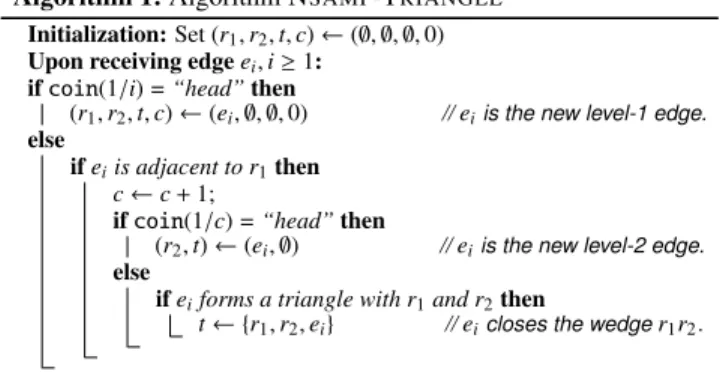
Algorithm 1:Algorithm NSAMP-TRIANGLE
Initialization:Set (r1,r2,t,c)←(∅,∅,∅,0)
Upon receiving edgeei,i≥1:
ifcoin(1/i)= “head”then
(r1,r2,t,c)←(ei,∅,∅,0) //eiis the new level-1 edge. else
ifeiis adjacent to r1then
c←c+1;
ifcoin(1/c)= “head”then
(r2,t)←(ei,∅) //eiis the new level-2 edge. else
ifeiforms a triangle with r1and r2then
t← {r1,r2,ei} //eicloses the wedger1r2.
We summarize the neighborhood sampling algorithm in Algorithm1 and analyze the probability that a triangle is sampled by the algo-rithm in the following lemma:
Lemma 3.1 Let t∗
be a triangle in the graph. The probability that t=t∗
in the state maintained by Algorithm1after observing all edges (note t may be empty) is
Pr[t=t∗]= 1
m·C(t∗)
where we recall that C(t∗
)=c(f)if f is t∗
’s first edge in the stream.
PROOF. Lett∗ ={
f1,f2,f3}be a triangle in the graph, whose edges arrived in the orderf1,f2,f3in the stream, soC(t∗)=c(f1) by definition. LetE1be the event thatf1is stored inr1, andE2be the event thatf2is stored inr2. We can easily check that neighborhood sampling producest∗
if and only if bothE1andE2hold.
Now we know from reservoir sampling thatPr[E1]= m1. Further-more, we claim thatPr[E2|E1]= c(1f
1). This holds because given
the eventE1, the edger2 is randomly chosen fromN(f1), so the probability thatr2=f2is exactly 1/|N(f1)|, which is 1/c(f1), since
ctracks the size ofN(r1). Hence, we have
Pr[t=t∗ ] = Pr[E1∩ E2]=Pr[E1]·Pr[E2| E1] = 1 m· 1 c(f1) = 1 m·C(t∗)
3.2
Counting Triangles
For a given trianglet∗∈ T
(G), neighborhood sampling produces
t∗
with probability 1
mC(t∗). To estimate the number of triangles, we first turn this into a random variable with the correct expectation: Lemma 3.2 Let t and c be the values the neighborhood sampling algorithm maintains, and m be the number of edges observed so far. Define ˜ τ= c×m if t,∅ 0 otherwise. Then,E[˜τ]=τ(G).
PROOF. By Lemma3.1, we sample a particular trianglet∗ with probabilityPr[t=t∗
]= 1
mC(t∗). Sincec=C(t), we have that ift=t ∗
, then ˜τ=mC(t∗
). Therefore, the expected value of ˜τis E[˜τ]= X
t∗∈T(G)
Given an estimate with the right expected value, to obtain good accuracy with a high enough probability, we keep multiple inde-pendent copies of the estimate and aggregate them. The following theorem answers the question: how many such estimates are suffi-cient to obtain an (ε, δ)-approximation?
Theorem 3.3 (Triangle Counting) Let0 < δ, ε ≤ 1and r ≥ 1. There is a streaming algorithm using O(r)space that on an arbitrarily-ordered stream of any graph G, returns an(ε, δ)-approximation to the triangle count in G, provided that r≥ 6
ε2 m∆ τ(G)log 2 δ . PROOF. Letα = 6 ε2 m∆ τ(G)log 2 δ
. We show that the average of
r≥αindependent unbiased estimates from Lemma3.2is an (ε, δ )-approximation. Fori = 1, . . . ,r, letXi be the value of thei-th estimate. Let ¯X=1rPri=1Xidenote the average of these estimators. Then, by Lemma3.2, we haveE[Xi] = τ(G) andE[ ¯X] = τ(G). Further, fore ∈ E, we havec(e) ≤2∆, so Xi ≤2m∆. LetYi =
Xi/(2m∆) so thatYi ∈ [0,1]. By lettingY = Pr
i=1Yi, we have E[Y]=r·τ(G)/(2m∆). Thus, we have thatPrhX¯ >(1+ε)E[X]iis at most PrhP iYi>(1+ε)E[Y] i ≤e−ε 2 3E[Y]≤δ/2
by Chernoff bound (Theorem2.1). Similarly, we can show that Pr[X<(1−ε)E[X]]≤δ/2. Hence, with probability at least 1−δ, the average ¯Xapproximates the true count within 1±ε. Since each estimator only takesO(1) space, the total space isO(r).
3.2.1
A Sharper Space Bound For Triangle Counting
The sufficient condition in the previous theorem is rather con-servative. In practice, we tend to observe much better results than the theorem suggests. We now show a sharper bound on the space requirement by being more precise about the spectrum of thec(·) values. Toward this goal, we define a measure that captures the amount of interaction between triangles and non-triangle edges in the graph. Thetangle coefficientof a graphG, denoted byγ(G), is given by γ(G) := 1 τ(G) X t0∈T(G) C(t0) or equivalently,γ(G)= τ(1G)P
e∈Ec(e)s(e), wheres(e) counts the number of trianglest0 ∈ T
(G) such that the first edge oft0 ise. Using the tangle coefficient, we prove the following theorem, which gives a different way to aggregate the results of different unbiased estimators (we briefly discuss the intuition behind tangle coefficient after that):
Theorem 3.4 (Improved Triangle Counting) Letγ(G)denote the tangle coefficient of a graph G. Let0< δ, ε≤1and r≥1. There is a streaming algorithm using O(r)space that on an arbitrarily-ordered stream of any graph G, returns an(ε, δ)-approximation to the triangle count in G, provided that r≥48
ε2 mγ(G) τ(G) log 1 δ .
PROOF. First, we note that an estimator in Lemma3.2has vari-ance at mostmP
t∈T(G)C(t)=m·τ(G)γ. We will runα=4/ε 2·
γm/τ(G) independent parallel copies of such an estimator. Let the average of these estimates beY. By Chebyshev’s inequality, we havePr[|Y−E[Y]|> ε·τ(G)]≤1
4.To increase the success prob-ability to 1−δ, we will runβ=12 ln(1/δ) independent copies of
Y estimators and take the median. Hence, our median estimator fails to produce anε-approximation only if more thanβ/2 fails to produce anε-approximation. In expectation, the number of “failed” estimators is at mostβ/4. Therefore, by a Chernoff bound (The-orem2.1), it fails with probability at most exp(−12(β/4)
3 )=δ. We
conclude that the final estimate is an (ε, δ)-approximation using at mostO(αβ) space.
Notice that the tangle coefficientγis at most 2∆, recovering the original bound we proved. Butγis often much smaller than that, especially in graphs such as power-law graphs, where there are only a few vertices with degree close to∆and the degrees of rest of the vertices are much smaller than∆. We can gain more understanding of the tangle coefficientγby considering the following random process: Fix a stream and pick a random triangle from this graph. If
eis the first edge in the stream of this triangle, then the value ofγis the number of edges that are adjacent toeand come aftere. In this view,γcan be seen as a measure of how entangled the triangles in this stream are—as our intuition suggests, if the triangles “interact” with many non-triangle triples, we will need more space to obtain an accurate answer.
3.3
Nearly-Linear Time Triangle Counting
Our discussion thus far directly leads to a simpleO(mr)-time implementation, whereris the number of estimators being main-tained; however, this can be too slow for large graphs. We want the algorithm to take time linear in the number of edgesmand the number of estimatorsr.
This section describes a bulk-processing scheme that delivers sig-nificantly better performance than the na¨ıve implementation. Bulk processing helps because the estimators need to be updated much less often. It also represents a common usage pattern: in many applications, the algorithm receives edges in bulk (e.g., block reads from disk) or has infrequent queries compared to updates (e.g., users only make queries every once in a while, so the incoming changes can be queued up). We show the following bounds:
Theorem 3.5 (Bulk Processing) Let r≤m be the number of esti-mators. There is an algorithmbulkTCfor triangle counting that processes a batch of w edges in time O(r+w). Furthermore, at any point in time, the algorithm needs at most O(r+w)space.
As a corollary, using a batch size ofw=Θ(r), we can process
medges indm/webatches inΘ(m+r) total time usingO(r) space. That is, with a (small) constant factor increase in space, we are able to achieveO(m+r) time bound as opposed toO(mr).
3.3.1
Conceptual Overview
Suppose our estimators have already observed the streamS= he1, . . . ,emiand there is a batchB=hb1, . . . ,b|B|iof newly-arriving edges. We will devise an algorithm that simultaneously advances the states of allrestimators to the point after incorporating the batchB. Effectively, the states of therestimators will be as if they have observed the streamSconcatenated withB. The accuracy guarantees from the previous section follow directly because our process simulates playing these edges one by one in the same order. We will frequently refer to the prefixes ofB: To facilitate the discussion, letB(i)=hb
1, . . . ,bii(B(0)is the empty sequence), and for a sequence of edgesA, let degA(x) denote the degree of nodex
in the graph induced by the edge setA. Furthermore, we define two quantities:
c−(r)=|N(r)\B| and c+(r)=|N(r)∩B|
We remember that neighborhood sampling (Section3.1) main-tains for each estimator the following quantities: (1)r1—a uniformly-chosen random edge from the stream; (2)r2—a uniform sample fromN(r1); (3)t—a triangle if the edge closing the wedger1r2is found inN(r2); and (4)c=|N(r1)|. Conceptually, the batchBcan be incorporated as follows:
I J K L 1 2 3 4 5 I J K L degB(1)(afterKL) ∅ ∅ 1 1 degB(2)(afterJK) ∅ 1 2 1 degB(3)(afterIK) 1 1 3 1 degB(4)(afterIJ) 2 2 3 1 degB(5)(afterIL) 3 2 3 2
Figure 2: A 4-node streaming graph where a batch B =
hKL,JK,IK,IJ,ILiof 5 new edges (solid, labeled with their arrival order) is being added to a stream of 1 edge (dashed) which has arrived earlier—and the corresponding deg values as these edges are added. Degree values that change are circled.
Step 1:Resample Level-1 edges.If there weremedges prior to the batchBof sizew, for each estimator, keep the current edge with probability m
w+m, and with the remaining probability, replace it with an edge uniformly chosen fromB. We will also resetcto 0 if the level-1 edge is replaced.
Step 2:Identify Level-2 candidates and sample from them.For each estimator, the sample space we want to sample uniformly from is
N(r1). Given the currentr2, we know thatc−(r1) is the currentc (note that if the level-1 was replaced,cwas also reset to 0). Hence, we use the following rule to update Level-2 edges:
With probability c+(r1)
c−(r
1)+c+(r1), pick a random edge from
N(r1)∩B; otherwise, keep the currentr2. Moreover, the number of candidate edgescisc+(r1)+c−(r1).
Step 3:Detect edges that will close the wedges.For each estimator with level- 1 and 2 edgesr1andr2, we check if an edge inBthat comes afterr2can close the wedger1r2and updatetaccordingly.
3.3.2
An Efficient Implementation
We give an efficient implementation of the conceptual algorithm. The implementation maintainsrestimator statesest1, . . . ,estr, where eachesti maintainsesti.r1, esti.r2,esti.t, andesti.caccording to neighborhood sampling. When we store an edge, we also keep the position in the stream where it appears.
Implementing Step 1:In onerandInt(1,r+w) call, we can decide for each estimator whether to retain the current level-1 edge or which new edge inBto select. Thus, inO(r) time, all level-1 edges are properly updated. This is essentially a direct translation of the conceptual algorithm.
Implementing Step 2:Although conceptually rather simple, this step turns out to be the most involved part in the whole algorithm. The challenge is that we cannot afford to explicitly construct the candidate sets (ourrestimators can potentially have all different candidate sets). Instead, we need to navigate the input stream while implicitly tracking ther“substreams” simultaneously in spaceO(r+ w)—merely a constant factor more than the space needed to keep the estimator states and the newly-arrived edges alone.
The crux of our solution is an observation that characterizes the candidate set of a given level-1 edge (i.e.,N(r1)∩B) in terms of the degrees of the relevant nodes in the prefixes ofB. We state the observation first and explain it with examples after that:
Observation 3.6 For an edge e and a node w∈e, the set of edges in B incident to node w that comes after e is
Γ(e)(w)={b
i∈B:w∈biand degB(i)(w)> β(e)(w)}
whereβ(e)(w)=deg
B(k)(w)if e is bk∈B, orβ(e)(w)=0otherwise.
Therefore, for an edgee={x,y}, the set of edges inBadjacent toe
that come aftereis given byN(e)∩B=Γ(e)(x)∪Γ(e)(y).
To help understand this observation and subsequent descriptions, imagine adding the edges in Bone by one—b1,b2, . . . ,bw—and at every step, observe how the degrees of the nodes relevant toB
change; see Figure2for a running example. In this view,β(e)(w) is the degree of the nodewat the point when the edgeeis added. In our running example,β(JK)(K)=2 andβ(IK)(I)=1. Moreover, since JL<B, we haveβ(JL)(L)=0. Now, notice that as an edgee={x,y} is added, exactly two places in the degree vector change—i.e., the degrees ofxandyincrease by 1 (these are circled). Hence, ifbj∈B comes afterbi ∈ Band both are incident on a nodex, the degree ofxwhenbjis added is necessarily larger than that whenbiwas added—or mathematically, degB(j)(x) >degB(i)(x). Therefore, in
words, Observation3.6says that every edge incident onxwith a degree ofxhigher thanβ(e)(x) comes afterein the stream. To give some examples, consider thatβ(IK)(I)=1, so the edges incident onI that comes afterIKare exactly those with degB(i)(I)>1—that is,IJ
andIL. As another example, we know thatβ(IK)(K)=3, so there is no edge incident onKthat comes afterIKbecause none of the edges have degB(i)(K)>3.
Algorithm 2:edgeIter—a degree-keeping edge iterator
Bdeg[]– an array wheredeg[u]contains the degree of vertex
u, initially0. fori =1to|B|do
{x,y} ←bi
deg[x]=deg[x]+1 anddeg[y]=deg[y]+1
notify(EVENTA(i,{x,y},deg)).
notify(EVENTB(i,{x,y},x,deg[x])).
notify(EVENTB(i,{x,y},y,deg[y])). returndeg.
To apply the observation, we describe an edge iterator algorithm
edgeIter(Algorithm2) that maintains a table of the nodes’ degrees. The variabledegis initially an empty table and at the end of each iterationi,degcontains the degrees of all nodes present in B(i). Moreover, the algorithm generates the following two types of events as it rolls over the batch of edges:
EVENTA(i,{x,y},deg)—after going over the edge{x,y}at indexi, the current degree vector (degB(i)) isdeg.
EVENTB(i,{x,y},v,a)—after going over the edge{x,y}at indexi, the degree of nodevis now updated toa.
These events provide the “cues” needed to track the candidate sets for our estimators.
The implementation of Step 2 consists of three substeps:
B Step 2a: Calculate for eachesti with level-1 edge{x,y}, the values of β(r1)(x), β(r1)(y), deg
B(x) and degB(y); these quantities are sufficient to define implicitly the setN(r1)∩Baccording to Observation3.6. To accomplish this, we temporarily store two additional fields per estimator—β(r1)(x),β(r1)(y)—and make a table
L[] mapping L[i],i ∈ {1, . . . ,|B|}, to a list of estimators whose level-1 edge isbi (an “inverted index” of the estimators that just replaced their level-1 edges). Building this table takesO(r) time. Initially, setβ(r1)(x),β(r1)(y) to 0 for all estimators. Then, we run
edgeIterand onEVENTA(i,{x,y},deg), we go over the listL[i] and store in these estimators β(r1)(x) = deg
B(i)(x) = deg[x] and
β(r1)(y) = deg
B(i)(y) = deg[y]. When edgeIteris finished, its
return vector is degB. This can be implemented inO(r+w) time because the length of lists inL(i.e.P
i|L[i]|) isr.
BStep 2b:Pick the level-2 edges, each in terms of anEVENTB. With the information collected in 2a, Observation3.6fully defines the
sample space for level-2 edges in terms ofEVENTB’s. To illustrate, consider that in Figure2, the neighborhood of level-1 edgeIKis
N(IK)= {IJ,IL}. The edgeIJcreates twoEVENTB’s that we will use to identify it: EVENTB(4,{I,J},I,2) andEVENTB(4,{I,J},J,2). Likewise, the edgeILgenerates twoEVENTB’s:EVENTB(5,{I,L},I,3) andEVENTB(5,{I,L},L,2).
More generally, consider a level-1 edger1={x,y}. There area= degB(x)−β(r1)(x) edges inΓ(r1)(x), namely the edges corresponding toEVENTB(∗,∗,x, β(r1)(x)+1),. . .,EVENTB(∗,∗,x,deg
B(x)), where ∗denotes a wildcard match. Similarly, there areb = degB(y)−
β(r1)(y) edges inΓ(r1)(y), namely the edges corresponding toEVENTB
(∗,∗,y, β(r1)(y)+1),. . .,EVENTB(∗,∗,y,deg
B(y)). Thus, for each estimator, we havec−
(r1) = c(inherited from Step 1) andc+(r1)=a+b. Letϕ=randInt(1,c−+c+), where
c−=
c−
(r1) andc+=c+(r1) and translateϕas follows:
Algorithm 3:Translating edge numbers into events if(ϕ≤c−)thenkeep existingr
2
else if(ϕ≤c−+a)then
pick the edge that causesEVENTB(∗,∗,x, β(r1)(x)+ϕ−c−) else
pick the edge that causesEVENTB(∗,∗,y, β(r1)(y)+ϕ−c−−a)
BStep 2c:Convert the selection into actual edges. Each estimator
has decided which new edge, if any, is replacing the current level-2 edge but it is given in terms of anEVENTBevent. To convert these events into actual level-2 edges, we create a (hash) tableP[] mapping an ordered-pair (x,d) to a list of estimators that subscribe to the eventEVENTB(∗,∗,x,d) from the previous step. Then, we runedgeIterand onEVENTB, we consult the tablePto see which estimators, if any, selected this edge. Step 2c requiresO(r+w) time andPconsumes at mostO(r) space sinceP
`∈P|`| ≤r.
Implementing Step 3:We keep a (hash) tableQthat maps an edge needed to complete a triangle to the estimator(s) that needs it. This table can be populated by by looking at our estimator states. Once this table is constructed, we simply have to go through the edges in
Band check whetherbiis present inQand if so, whether it comes after the level-2 edge that expects it. This is easy to check because we store with every edge its position in the stream. Hence, Step 3 takes at mostO(r+w) time sinceQcan contain at mostrentries.
In sum, we have shown that each of these steps can be imple-mented inO(r+w) time using at mostO(r+w) space. Hence, the algorithmbulkTCsatisfies Theorem3.5, as promised.
3.4
Sampling Triangles
We now turn to the problem of maintainingk ≥1 triangle(s) uniformly-sampled with replacement from a graph stream. First, we show how to sample one triangle uniformly with a reasonable success probability. Following that, we apply it to samplek ≥1 triangles and outline how to adapt the efficient implementation (Section3.3) to this case.
Our starting point is the neighborhood sampling algorithm, which maintains a random triangle. The problem, however, is that this sam-ple is not necessarily uniform. But this is easy to fix, as described in the following lemma:
Lemma 3.7 Let G be a streaming graph. Let t and c be the values the neighborhood sampling algorithm maintains. Define
unifTri(G)= t with prob. 2c∆ ∅ otherwise.
Then,unifTri(G)produces a triangle (i.e.unifTri(G),∅) with probability at least τ2(mG∆). Furthermore, if it returns a triangle, each triangle inT(G)is equally likely to be produced.
PROOF. By Lemma3.1, neighborhood sampling picks a partic-ular trianglet∗ with probabilityPr[t=t∗] = 1/mC(t∗). Further, note thatC(t∗
)≤2∆. Therefore, if neighborhood sampling picks the trianglet∗
, the probability thatt∗
is passed on as our output is 1
mC(t∗)· C(t∗)
2∆ = 1
2m∆, where we note thatc=C(t ∗
) and the normaliza-tion factor c
2∆ ≤1. Finally, since the events of different triangles being returned are all disjoint from each other, the probability that some triangle is returned by the algorithm isτ2(mG∆).
We extend this to samplektriangles by running multiple copies
of unifTriand picking anyktriangles at random. Below, we
calculate the number of copies sufficient for producingktriangles with probability at least 1−δ.
Theorem 3.8 For0< δ <1, r≥1, and k≥1, there is an algorithm
unifTri(G,k)with space requirement O(r)that on any stream graph G withτ(G)>0, returns k triangles uniformly-chosen with replacement from G that succeeds with probability at least1−δ, as long as r≥4mk∆τ(ln(G)e/δ).
PROOF. We runr ≥ α = 4mk∆τln(e/δ)
(G) independent copies of
unifTri from Lemma3.7and randomly pickktriangles these
copies yield. Thus, it succeeds as long as at leastkcopies yield a triangle. To analyze this, letXbe the number of copies that yield a triangle and p=2m∆/τ(G) be a sampler’s success probability (Lemma3.7). Therefore,X is a Binomial random variable with meanαpbecause these are independent samplers succeeding with probability p. Hence, unifTri(G,k) succeeds with probability Pr[X≥k] = 1−Pr[X<k], wherePr[X<k] ≤exp(− 1
2αp(αp−
k)2)≤δ/e≤δby Chernoff bounds (Theorem2.1). We conclude that the algorithm succeeds with probability at least 1−δand con-sumesO(r) space because each copy takes constant space.
The algorithmunifTri(G,k) can also benefit from the bulk-processing implementation from Section3.3. Since Theorem3.5 im-plements neighborhood sampling for bulk arrival, the states it keeps are readily consumable by ourunifTrialgorithm (Lemma3.7). Hence, together with the theorem above, we have that as long as we keepr≥4mk∆τln(e/δ)
(G) , we can maintainkuniformly-sampled triangles in the same space/time bounds as Theorem3.5; that is,O(m+r) total time andO(r+w) space.
3.5
Transitivity Coefficient
Another important triadic graph measure is thetransitivity coeffi-cient, proposed by Newman, Watts, and Strogatz [15]:
κ(G)=3τ(G) ζ(G) , whereζ(G)=P u∈V(G) deg(u) 2
is the number of connected triplets in the graphG. Since we already have an algorithm for triangle counting, we will estimate the transitivity coefficient by designing an algorithm for estimatingζ(G). To start, we expressζ(G) in terms of a quantity related to what neighborhood sampling tracks: Claim 3.9 If c(e)is the number of edges incident on e that arrive after e in the stream, then
ζ(G)=X e∈E
PROOF. LetS = {{e,f} ⊆ E(G) : e , fand|e∩ f| =1}be the set of unordered pairs of edges that share a common vertex, so |S|=ζ(G). Further, letT={(p,q) : p∈ E(G) andq∈ N(p)}, so
|T|=P
e∈Ec(e). We prove the claim by giving a bijection between
SandT, showing that|S|=|T|. For this, we map each (p,q)∈Tto
{p,q} ∈S. It is routine to check that this mapping is well-defined and is bijective.
Using this relationship, we can estimateζ(G) as follows: Lemma 3.10 Let c be the quantity that neighborhood sampling tracks and m be the total number of edges seen so far. Define
˜
ζ=m×c. Then,Ehζ˜i=ζ(G).
PROOF. Fix an edgee∈E. Neighborhood sampling picks this edge as its level-1 edge with probability 1/mand when this edge is picked, the valuecis c(e), so ˜ζ = m×c(e). Thus,Ehζ˜i = P
e
1
mc(e)·m=ζ(G), which follows from Claim3.9.
Like in triangle counting, we boost the accuracy and success probability of the above estimator by running multiple copies and taking the average of the estimates. By Chernoff bounds (applied similarly to Theorem3.3), we have the following lemma:
Lemma 3.11 Let0≤δ, ε≤1. There is an algorithm that observes a graph stream G and returns an(ε, δ)-approximation forζ(G)using space O(1
ε2
m∆
ζ(G)log(1/δ)).
We put these together as follows: Run the triangle counting algo-rithm simultaneously with theζ-estimation algorithm. In particular, run the algorithm from Theorem3.3to computeτ0
(G), a (ε/3, δ/ 2)-approximation ofτ(G), and the algorithm from Lemma3.11to computeζ0(
G), a (ε/3, δ/2)-approximation ofζ(G)—and return
κ0
(G)=3τ0 (G)/ζ0
(G). Note that the total space used by this algo-rithm is bounded byO(1
ε2
m∆
ζ(G)log(1/δ)). By our choice of parameters and an application of union bound it follows thatκ0
(G)∈(1±ε)κ(G). Thus, we have the following theorem:
Theorem 3.12 Letε≤1, δ >0and r≥1. There is an O(r)-space
(ε, δ)-approximation streaming algorithm for transitivity coefficient, provided r≥ K
ε2
m∆
ζ(G)log(1/δ))for a fixed constant K.
3.6
A Lower Bound
It is natural to ask whether better space bounds are possible for triangle sampling and counting. In particular,can we meet the space complexity of O(1+T2(G)/τ(G)), which is the space-complexity of an
algorithm for triangle counting in the incidence stream model[5]? Here,T2(G) is the number of vertex triples with exactly two edges in them. We show that this space bound is not possible in the adjacency stream model, separating it from the incidence stream model: Theorem 3.13 There exists a graph G∗
and an order of arrival of edges, such that any randomized streaming algorithm that can estimate the number of triangles in G∗
with a relative error of better than1/2must have space complexityω(1+T2(G)/τ(G)).
PROOF. We use a reduction from theIndexproblem from com-munication complexity: Alice is given a bit vectorx∈ {0,1}nand Bob is given an indexk∈ {1,2, . . . ,n}; Bob wants to computexk, the bit in thek-th position inx. It is known that in the model where Alice can send exactly one message to Bob, the communication cost of any (randomized) protocol isΩ(n) bits (see [11, Chapter 4.2]).
LetAbe a streaming algorithm that estimates the number of trian-gles. We can use this algorithm to solve theIndexproblem as follows.
Given a bit vectorx∈ {0,1}n, Alice constructs a graphG∗
on 3(n+1) vertices with the vertex set{a0,· · ·,an} ∪ {b0,· · ·,bn} ∪ {c0,· · ·,cn}; the edges are as follows: she forms a triangle ona0,b0,c0—and for eachi∈ {1,2, . . . ,n}, she places the edge (ai,bi) if and only if
xi=1. Alice processes this graph usingAand sends the state of the algorithm to Bob, who continues the algorithm using the state sent by Alice, and adds the two edges (bk,ck) and (ck,ak), wherekis the index requested. By querying the number of triangles in this graph with relative error of smaller than 1/2, Bob can distinguish between the following cases: (1)G∗
has two triangles, and (2)G∗ has one triangle. In case (1),xk=1 and in Case (2),xk=0, and hence, Bob has solved theIndexproblem.
It follows that the memory requirement of the streaming algorithm an Alice’s end must beΩ(n) bits. Note that the graphG∗
sent by Alice has no triples with two edges between them, and hence,
O(1+T2(G∗)/τ(G∗))=O(1).
4.
EXPERIMENTS
In this section, we empirically study the accuracy and the runtime performance of the proposed triangle counting algorithm on real-world, as well as synthetic, graphs and in comparison to existing streaming algorithms.
We implemented the version of the algorithm which processes edges in batches and also the other state-of-the-art algorithms for ad-jacency streams due to Buriol et al. [5], and Jowhari and Ghodsi [9]. Our bulk-processing algorithm follows the description in Section3.3, with the following optimizations: First, we combine Steps 2c and 3 to save a pass through the batch. Second, level-1 maintenance can be further optimized by noticing that in later stages, the number of estimators that end up updating their level-1 edges is progressively smaller. Deciding which estimator gets a new edge boils down to generating a binary vector wherepis the probability that a position is 1 (as time progresses,pbecomes smaller and smaller). We can generate this by generating a few geometric random variables repre-senting the gaps between the 1’s in the vector. Since we expect only ap-th fraction of the estimators to be updated, this is more efficient than going over all the estimators. Our implementation uses GNU’s STL implementation of collections, includingunordered_mapfor hash maps; we have only performed basic code optimization.
4.1
Experimental Setup
Our experiments were performed on a 2.2 Ghz Intel Core i7 laptop machine with 8GB of memory, but our experiments only used a fraction of the available memory. The machine is running Mac OS X 10.7.5. All programs were compiled with GNUg++
version 4.2.1 (Darwin) using the flag-O3. We measure and report wall-clock time usinggettimeofday.
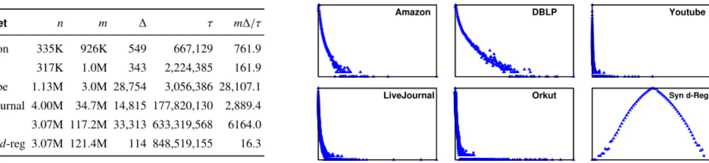
We use a collection of popular social media graphs, obtained from the publicly available data provided by the SNAP project at Stanford [12]. We present a summary of these datasets in Figure3. We remark that while these datasets stem from social media, our algorithm does not assume any special property about them. Since these social media graphs tend to be power-law graphs, we comple-ment the datasets with a randomly-generated synthetic graph (called “Synthetic∼d-regular”) that has about the same number of nodes and edges as our biggest real dataset (Orkut)—but the nodes have degrees between 42 and 114.
The algorithms considered are randomized and may behave dif-ferently on different runs. For robustness, we performfivetrials with different random seeds and report the following statistics:(1)the mean deviation (relative error) values from the true answer across the trials,(2)the median wall-clock overall runtime, and(3)the median I/O time. Mean deviation is a well accepted measure of
Dataset n m ∆ τ m∆/τ Amazon 335K 926K 549 667,129 761.9 DBLP 317K 1.0M 343 2,224,385 161.9 Youtube 1.13M 3.0M 28,754 3,056,386 28,107.1 LiveJournal 4.00M 34.7M 14,815 177,820,130 2,889.4 Orkut 3.07M 117.2M 33,313 633,319,568 6164.0 Syn.∼d-reg 3.07M 121.4M 114 848,519,155 16.3 Amazon DBLP Youtube
LiveJournal Orkut Syn d-Reg
Figure 3:A summary of the datasets used in our experiments: the left panel shows for every dataset the number of nodes (n), the number of edges (m), the maximum degree (∆), the number of triangles in the graph (τ), and the ratiom∆/τ; the right panel shows for each dataset, a plot of frequency (vert. axis in log scale) vs. degree (linear scale).
error, which we believe to give an accurate picture of how well the algorithm performs. For some experiments, we also report the min/max deviation values for completeness, but we note that as more trials are performed, the minimum becomes smaller and the maximum becomes larger, so they are not robust.
4.2
Baseline Study
The state-of-the-art algorithms for adjacency streams are due to Buriol et al. [5], and Jowhari and Ghodsi [9]; we discuss their performance in turn.
Our implementation of Buriol et al.’s algorithm follows the de-scription of the optimized version in their paper, which achieves roughlyO(m+r) running time formedges andrestimators through certain approximations. Even though the algorithm is fast, it fails to find a triangle most of the time, resulting in low-quality estimates, or producing no estimates at all—even when using millions of es-timators on the large graphs that we consider (see Section3.1for a related discussion); this is consistent with Buriol et al.’s findings about the adjacency stream algorithm [5]. Hence, we do not report further results on this algorithm.
Our implementation of Jowhari-Ghodsi’s algorithm follows the description in their paper, which achievesO(mr) total running time. It is, however, too slow for extensive experiments on the datasets in Figure3. Hence, we use smaller datasets to compare with our algorithm:
— Syn3-regis a 3-regular graph withn=2,000 nodes;m=3,000 edges, and a max. degree of∆ = 3, containingτ = 1,000 triangles.
— Hep-This an arXiv Hep-Th collaboration network [12] with
n=9,877 nodes;m=51,971 edges;∆=130 max. degree with
τ=90,649 triangles.
The results are shown in Tables1and2. On the synthetic 3-regular graph, which has very smallm∆/τ=9, both algorithms give accurate estimates yielding better than 92% accuracy even with only
r=1,000 estimators. Both yield progressively better estimates with more estimators with JG being more accurate. However, our bulk-processing algorithm is at least 10x faster. On theHep-Thgraph, which hasm∆/τ = 74.53, neither algorithms is able to produce a reasonable estimate across 5 runs withr = 1,000 or 10,000. But withr =100,000 estimators, our algorithm’s error drops to below 1% while we see no improvements from JG. Again, the bulk-processing algorithm is at least 10x faster. Importantly, we note that for the same value ofr(number of estimators), the JG algorithm uses considerably more space than our algorithm, since our algorithm uses constant space per estimator while the JG algorithm uses up to
O(∆) space per estimator.
Algorithm r=1,000 r=10,000 r=100,000
MD Time MD Time MD Time
JG [9] 7.20 0.04 2.08 0.44 0.27 5.26
Ours 4.28 0.004 1.52 0.01 0.93 0.07
Table 1: The accuracy (mean deviationin percentage) and pro-cessing time (in seconds) of Jowhari-Ghodsi(JG)’s algorithm in comparison to our algorithm on a synthetic 3-regular graph (Syn.
3-reg) as the number of estimators is varied.
Algorithm r=1,000 r=10,000 r=100,000
MD Time MD Time MD Time
JG [9] 79.33 0.71 86.86 7.17 86.66 86.02
Ours 92.69 0.05 81.25 0.08 0.68 0.17
Table 2: The accuracy (mean deviationin percentage) and pro-cessing time (in seconds) of Jowhari-Ghodsi(JG)’s algorithm in comparison to our algorithm onHep-Thas the number of estimators is varied.
These findings suggest thatexisting algorithms for adjacency streams can deliver accurate results but require more estimators, memory, and runtime for obtaining results of similar quality as our algorithm, and hence are impractical for large graphs.In the remaining experiments, we directly compare our results with the true count to assess accuracy and study the scalability of the approach as the graph size and the number of estimators increase.
4.3
Accuracy, Speed, and Memory Usage
This set of experiments aims to study the accuracy, speed, and memory usage of our estimates on different datasets. Our theoretical results predict that as the number of estimatorsrincreases, so does the accuracy. We are interested in verifying this prediction, as well as studying the dependence of the accuracy on parameters such as the number of edgesm, maximum degree∆and the number of trianglesτ.
For each dataset, we run 5 trials of the bulk-processing algorithm withr=1024, 131072, and 1048576. The number of estimators (r) controls the memory requirement for keeping the states. Our implementation uses 36 bytes per estimator; therefore, regardless of the datasets, the memory usage for the estimators is as follows:
r=1K r=128K r=1M
Memory 36K 4.5M 36M
In addition, when a batch of edges arrives, the bulk-processing algorithm needs a working space of about 3x the batch size to process the batch; this space is thrown away after it completes the batch. We further discuss the effects of batch size in Section4.5.
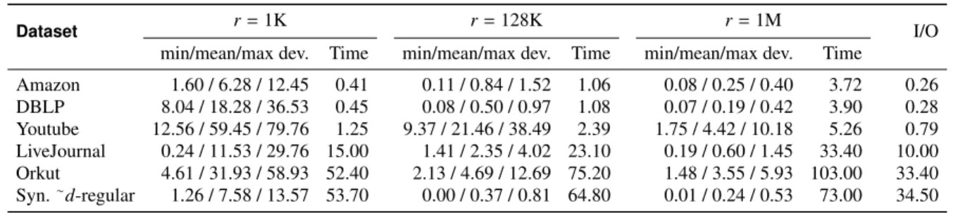
Dataset r=1K r=128K r=1M I/O min/mean/max dev. Time min/mean/max dev. Time min/mean/max dev. Time
Amazon 1.60 / 6.28 / 12.45 0.41 0.11 / 0.84 / 1.52 1.06 0.08 / 0.25 / 0.40 3.72 0.26 DBLP 8.04 / 18.28 / 36.53 0.45 0.08 / 0.50 / 0.97 1.08 0.07 / 0.19 / 0.42 3.90 0.28 Youtube 12.56 / 59.45 / 79.76 1.25 9.37 / 21.46 / 38.49 2.39 1.75 / 4.42 / 10.18 5.26 0.79 LiveJournal 0.24 / 11.53 / 29.76 15.00 1.41 / 2.35 / 4.02 23.10 0.19 / 0.60 / 1.45 33.40 10.00 Orkut 4.61 / 31.93 / 58.93 52.40 2.13 / 4.69 / 12.69 75.20 1.48 / 3.55 / 5.93 103.00 33.40 Syn.∼ d-regular 1.26 / 7.58 / 13.57 53.70 0.00 / 0.37 / 0.81 64.80 0.01 / 0.24 / 0.53 73.00 34.50 Table 3:The accuracy (min/mean/max deviationin percentage), median total running time (in seconds), and I/O time (in seconds) of our bulk algorithm across five runs as the number of estimatorsris varied.
0 1 2 3 4 5 6 7 8
Amazon DBLP Youtube LiveJournal Orkut
Average Throughput (Mil. Edges Per Second)
with r=1K with r=128K with r=1M
Figure 4:Average throughput of the streaming algorithm (in mil-lion edges per second) on different real-world datasets as the num-ber of estimators is varied.
Table3shows the median total running time, accuracy (showing min., mean, and max. relative errors in percentage), and median I/O time of our algorithm across five runs as we vary the number of estimatorsr. We show the I/O time for each dataset as it makes up of a non-negligible fraction of the total running time. Several things are clear from this experiment in terms of accuracy: First,our algorithm is accurate with only a modest number of estimators. In all but the Youtube dataset, the algorithm achieves less than 5% mean deviation using only about 100 thousand estimators. Furthermore, the accuracy significantly improves as we increase the number of estimatorsrto 1M. Second,a high degree graph with few triangles needs more estimators. Consistent with the theoretical findings, Youtube and Orkut, which have the largestm∆/τ(G) values, need more estimators than others to reach the same accuracy. Third, but perhaps most importantly,in practice, far fewer estimators than suggested by the pessimistic theoretical bound is necessary to reach a desired accuracy. For example, on Orkut, usingε = 0.0355, the expressions(ε, δ)m∆/τis at least 4.89 million, but we already get this accuracy using 1 million estimators. Finally, we note that across the datasets,the mean deviation decreases as we increase the number of estimators.This is desirable and to be expected; as the proof suggests, the aggregate becomes progressively sharper as we increase the number of estimators.
Power-law or not.Our real-world datasets stem from social media, which tend have a power-law degree distribution. It is natural to wonder how the scheme performs on non-power-law graphs. For this, we experimented with a synthetic graph of roughly the same size as Orkut. The result on the synthetic graph suggests that as long asm∆/τis small, our algorithm is capable of producing accu-rate results—regardless of the power-law nature. In more “regular”
graphs, we believe thatm∆/τwill be a better predictor of accuracy because the degree variance is smaller.
Having discussed the accuracy and memory usage trends, we now turn to the throughput of the algorithm. Figure4shows the average throughput of our algorithm for different real-world datasets as the number of estimators is varied. These numbers represent the throughput we obtain on average for processing a stream of edges of a particular length. Since the I/O rate is faster than the processing rate and we factor out the I/O time, these are the highest “sustained” rate the algorithm can achieve on that stream. As expected, the throughput decreases as the number of estimators increases (which yields more accuracy). Furthermore, for a fixedr(and using, say,
w=8r), the throughput increases with the stream’s length: since the total time to process a stream of lengthmis proportional tom+r, the throughput is proportional to m
m+r =
1
1+r/m, which increases withm. We focus onr=128K andr=1M as these are likely the values one is likely to use to obtain an accurate estimate. Withr=128K, the algorithm is capable of handling more than 1 million edges/second— and withr=1M, for sufficiently long streams, it can process more than 1.2 million edges/second.
4.4
Effects of The Number of Estimators
In this set of experiments, we selected two graphs—Youtube and LiveJournal—to study the algorithm’s behaviors in more detail.
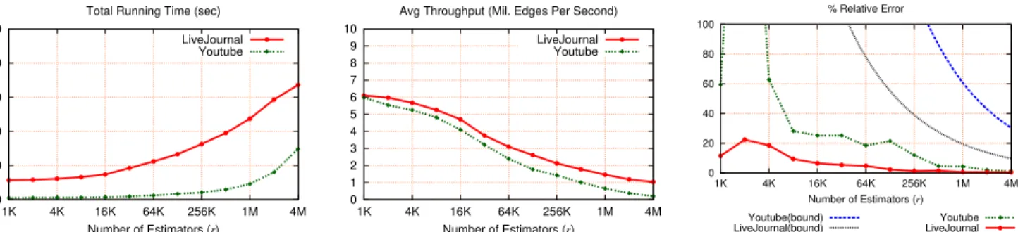
Figure5(left) shows the median running time (in seconds) asr
geometrically increases fromr=1024 tor=4M; the horizontal axis (x-axis) is in log scale. This translates into the average through-put curves in the middle panel. As can be seen, the running time increases with the number of estimatorsr, as expected. The theory predicts that the running time isO(m+r); that is, it scales linearly withr. This is hard to confirm visually since we do not know how much of it is due to theO(m) term; however, in both cases, we are able to compute a valuet0such that the running times minust0scale roughly linearly withr, suggesting that the algorithm conforms to theO(m+r) bound.
We also study the mean deviation asrchanges. Figure5(right) shows the mean deviation values for the same two datasets as well as the error bound indicated by Theorem3.3usingδ=1/5. Ignoring the first several data points where using a small number of estimators results in low accuracy and high fluctuations, we see that in general— though not a strict pattern—the error decreases with the number of estimators. Furthermore, consistent with our earlier observations, the bound in Theorem3.3is conservative; we do better in practice.
4.5
Effects of Batch Size
In this section, we discuss the effects the batch size have on memory consumption and the processing throughput. When a batch of edges arrives, the bulk-processing algorithm needs a working space of about 3x the space for storing the arriving edges to process the batch this space is thrown away after it completes each batch.
0 10 20 30 40 50 1K 4K 16K 64K 256K 1M 4M Number of Estimators (r)
Total Running Time (sec)
LiveJournal Youtube 0 1 2 3 4 5 6 7 8 9 10 1K 4K 16K 64K 256K 1M 4M Number of Estimators (r)
Avg Throughput (Mil. Edges Per Second)
LiveJournal Youtube 0 20 40 60 80 100 1K 4K 16K 64K 256K 1M 4M Number of Estimators (r) % Relative Error Youtube(bound) LiveJournal(bound) Youtube LiveJournal
Figure 5:(Left) running time (in seconds), (center) average throughput (in million edges per second), (right) mean deviation (in percentage) as as the number of estimatorsris varied (r=1K,2K, . . . ,4M). Thex-axis is in log scale.
0 0.2 0.4 0.6 0.8 1 1.2 1.4 1 2 3 4 5 6 7 8
Avg Throughput (million edges per sec)
Batch Size (in millions) LiveJournal
Figure 6: The throughput of the bulk-processing algorithm on LiveJournal as the batch size is varied.
As an example, using a batch size ofw=8M and 1M estimators, the implementation would have a high water mark around 164MB. Furthermore, we study the effects on the throughput by performing an experiment on LiveJournal graph withr = 1M, varying the batch size between 1M and 8M. The results are shown in Figure6, suggesting that the throughput increases with the batch size. This agrees with the running time bound we derived in Theorem3.5: the average time to process an edge in a stream of lengthmis proportional to 1+ r m + w m+ 1 w.
5.
EXTENSIONS
In this section, we demonstrate the versatility of the neighborhood sampling technique by using it to derive a space-efficient streaming algorithm for counting higher-order cliques, as well as applying it to the problem of triangle counting in a sliding window model. These results are mostly of theoretical interest.
5.1
Counting and Sampling Cliques
For ease of presentation, we focus on 4-cliques. LetT4(G) denote the set of all 4-cliques inG, andτ4(G) the number of 4-cliques inG. The most crucial ingredient of our triangle counting algo-rithm is the neighborhood sampling subroutine. Following the same recipe for estimating 4-cliques, our first step would be to design a neighborhood sampling algorithm for 4-cliques. Given a proper neighborhood sampling algorithm, it is easy to obtain an unbiased estimator, and taking the average of multiple copies of the unbiased estimator yields a good estimate for the number of 4-cliques.
Extending neighborhood sampling to 4-cliques requires extra care, however. In the case of triangles, we first sample an edger1, and then samples a neighbor fromN(r1), and waits for the arrival
of the third edge that completes the triangle. A natural extension to 4-cliques is to sample an edger1, sampler2fromN(r1), and sampler3from the set of neighbors ofr1andr2that arrive after
r2—then, wait for the remaining edges to complete the 4-clique. Unfortunately, this strategy will miss many 4-cliques: Consider a 4-cliqueκ∗={
f1,f2,f3,f4,f5,f6}whose edge arrive in that order. If
f1and f2do not share a vertex, the above strategy will never sample
κ∗
. However, we would like our neighborhood sampling algorithm to pick each 4-clique with a non-zero probability.
We overcome this difficulty by partitioning the set of 4-cliques into two classes—Type IandType II—and design two neighbor-hood sampling algorithms to estimate their numbers separately. The type of a 4-clique is determined by the order its edges appear in the stream. Let f1, . . . ,f6 be the edges of a 4-cliqueκ∗ arriving in that order. We say thatκ∗
is aType Iclique if f2and f1share a common vertex; otherwiseκ∗
is aType IIclique. Thus, every
clique is, by definition, eitherType IorType II. LetT1
4(G) be the set ofType Icliques inGandT2
4(G) be the set ofType IIcliques; letτ1
4(G) andτ 2
4(G) denote the corresponding sizes.
For sampling purposes, the basic distinction betweenType Iand
Type IIcliques is as follows: Let f1, . . . ,f6 be the edges of a 4-cliqueκ∗
arriving in that order. Ifκ∗
is aType Iclique, since f1and
f2share a vertex, three of the first four edges (f1,f2and one of f3 or f4) determine all four vertices of the clique. Ifκ∗is aType II clique then the first two edges (f1,f2) determine all four vertices of the clique.
5.1.1
Neighborhood Sampling for 4-Cliques
Letf1andf2be two edges ofS, wheref2arrives after f1. LetF be the set of edges adjacent to both f1and f2(possibly empty). The neighborhood of f1and f2, denoted byN(f1,f2), is
N(f1,f2)={e∈N(f1)|ecomes after f2} ∪N(f2)−F, and letc(f1,f2) denote the size ofN(f1,f2).
Neighborhood sampling forType Icliques.As mentioned earlier, we need three edges to determine all vertices of aType Iclique. Thus, our sampling algorithm maintains a sample of three edges over four vertices and looks for edges that complete the 4-clique. Our algorithm maintains following states:
— level-1 edger1, level-2 edger2, level-3 edger3—r1is uniformly sampled from all the edges seen so far;r2is drawn at random fromN(r1);r3is drawn at random fromN(r1,r2).
— countersc1andc2—c1tracks the size ofN(r1) andc2tracks the size ofN(r1,r2).
— potential clique κ1—edges of a potential clique that can be formed using edgesr1,r2, andr3.
We use the standard reservoir sampling technique to pickr1,r2 andr3. We present a more detailed description in Algorithm4.