Using Automated Planning for Improving Data Mining Processes

(1)

DOI: 10.1017/S000000000000000

Printed in the United Kingdom

Using Automated Planning for Improving Data Mining

Pro-cesses

Susana Fern´

andez

1

, Tom´

as de la Rosa

1

, Fernando Fern´

andez

1

, Rub´

en Su´

arez

1

,

Javier Ortiz

1

_{, Daniel Borrajo}

1

_{, and David Manzano}

2

1_{Universidad Carlos III de Madrid. Legan´}_{es (Madrid). Spain} 2_{Ericsson Research Spain. Madrid, Spain}

Abstract

This paper presents a distributed architecture for automating data mining processes using standard languages. Data mining is a difficult task that relies on an exploratory and analytic process of processing large quantities of data in order to discover meaningful patterns. The increasing heterogeneity and complexity of available data requires some expert knowledge on how to combine the multiple and alternative data mining tasks to process the data. Here, we describe data-mining tasks in terms of Automated Planning, which allows us to automate the data-mining knowledge flow construction. The work is based on the use of standards that have been defined in both data mining and automated-planning communities. Thus, we use PMML (Predictive Model Markup Language) to describe data mining tasks. From the PMML, a problem description in PDDL (Planning Domain Definition Language) can be generated, so any current planning system can be used to generate a plan. This plan is, again, translated to a data-mining workflow description, KFML format (Knowledge Flow file for the WEKA tool), so the plan or data-mining workflow can be executed in WEKA (Waikato Environment for Knowledge Analysis).

1 Introduction

Currently, many companies are extensively using Data-Mining (DM) tools and techniques. DM deals with the development of methods and techniques for analyzing data. The data or dataset is represented as a set of patterns described in terms of features. The first step of the DM process is usually related to the selection, pre-processing and transformation of the data to be analyzed. The following step consists of applying data analysis and discovery algorithms to generate models that describe the data (Fayyad, et al. 1996). It commonly involves four classes of task: classification, clustering, regression or association rule learning. The DM process finishes with the interpretation and evaluation of the models. The evaluation of a DM problem typically involves applying the new model to data that was not used to generate the model. Depending on the amount of data, or the type of function to be modelled, different evaluation approaches may be used. Therefore, in the DM process, there are four main elements to define: the training data (obtained by selecting, pre-processing, and transforming the initial dataset), the model or language representation, the learning algorithm, and how to evaluate the model. The number of combinations of those four elements is huge, since there are many different methods and techniques appropriate for each phase, all of them with different parameter settings, which can be applied in different orders. Thus, the DM process is sometimes seen as an expert process where DM engineers transform original data, execute different mining operators, evaluate the obtained models, and repeat this process until they are satisfied. The complexity of this combinatorial process suggests using automated

(2)

approaches (Michalski & Kaufman 1998, Fern´andez, et al. 2009, Kietz, et al. 2009, Diamantini, et al. 2009, Bernstein, et al. 2005, Zakova, et al. 2008).

In this paper, we present an architecture and a tool based on Automated Planning (AP) that helps users (non necessarily experts on DM) to perform DM tasks. The starting point will be a definition of the DM task to be carried out and the output will be a set of plans that are executed in a DM tool to obtain a set of models and statistics. In order to define the DM task, we use emerging standards, such as PMML (Predictive Model Markup Language). PMML is the leading standard for statistical and data mining models and supported by over 20 vendors and organizations. With PMML, it is straightforward to develop a model on one system using one application and deploy the model on another system using another application. The PMML file is automatically translated into a planning problem described in PDDL (the standard language in the planning community). So, any state-of-the art planner can be used to generate a plan (or plans), i.e. the sequence of DM actions that should be executed over the initial dataset to obtain the final model. Each plan or knowledge flow is executed by a machine learning engine after translating the plan from the planner output-format into the DM engine input-format.

In our case, we employ one of the most used DM tools, WEKA (Witten & Frank 2005). In WEKA, knowledge flows are described as files with a specific format, KFML, and datasets are described as ARFF (Attribute-Relation File Format) files. The results of the DM process can be evaluated, and new plans may be requested from the planning system.

In order to understand the complexity of the DM tasks, WEKA implements more than 50 different transformation actions or filters (pre-processing techniques), more than 40 training actions for classification and regression, and 11 training actions for clustering. Each of these transformation and training actions can be parameterized (with many continuous parameters), so the number of different instantiations of those actions can potentially be infinite (or huge if we perform some kind of discretization of continuous parameters of DM techniques). Also, there can be potentially many transformations that can be applied to the data before training, and there is no limit on the number of applicable transformations. Finally, the order in which actions are applied is quite relevant to the final results. For instance, it is not the same applying a discretization to all attributes before performing attribute selection, than performing first an attribute selection and then a discretization, since the attribute selection technique might generate different subsets of attributes depending on the representation of the attributes. Precisely, AP technology has become mature enough to be useful in applications that require selecting and sequencing actions (Ghallab, et al. 2004), such as solving DM problems. The reason why it is a planning problem instead of a Constrain Satisfaction Problem is because the order matters, as the previous example shows.

The remaining sections describe the languages used in the application, the general architecture, the modelling of the DM tasks in PDDL, the planning process, the generation of the DM models, the experiments, the related work and the conclusions.

2 Use of Standard Languages

In this work we have used three different languages: PMML (Predictive Model Markup Language), an XML based language for DM; KFML (Knowledge Flow for Machine Learning), another XML based language to represent DM knowledge flows for the WEKA tool (Witten & Frank 2005); and PDDL (Planning Domain Definition Language), the standard AP language.

PMML is a markup language for describing statistical and DM tasks and models. It is based on XML, and it is composed of five main parts:

• The header contains general information about the file, like the PMML version, date, etc.

• The data dictionary defines the meta-data, or the description of the input data or learning examples.

• The transformation dictionary defines the applicable functions over the input data, like flattening, aggregation, average or standard deviation computation, normalization, principal

(3)

component analysis (PCA), etc. This knowledge defines the actions that can be applied over the data in the first step of the mining process.

• The models contain the definition of the DM model. For instance, a multi-layered feed-forward neural network is represented in PMML by a “NeuralNetwork” element which contains attributes such as: a Model Name (attribute modelName), a Function Name (attribute functionName), an Algorithm Name (attribute algorithmName), an Activation Function (attribute activationFunction), and a Number of Layers (attribute numberOfLayers). This information is then followed by three kinds of neural layers which specify the architecture of the neural network model being represented in the PMML document. These attributes are NeuralInputs, NeuralLayer, and NeuralOutputs. Besides neural networks, PMML allows for the representation of many other DM models including support vector machines, association rules, bayesian classifiers, clustering models, text models, decision trees, and different regression models.

• The mining build task describes the configuration of the training task that will produce the model instance. This mining build task can be seen as the description of the sequence of actions executed to obtain the model, so from the perspective of planning, it can be understood as a plan. Therefore, the goal of the planning process is to automatically generate this section.

WEKA (Witten & Frank 2005) is a collection of machine learning algorithms to perform DM tasks. It incorporates the WEKA Knowledge Flow, that allows to build a knowledge flow for processing and analysing data. Such knowledge flow can include most of WEKA functionalities: load data, prepare data for cross-validation evaluation, apply filters, apply learning algorithms, show the results graphically or in a text window, etc. Knowledge flows are stored in KFML files, that can be given also as input to WEKA. A KFML file is an XML file including two sections. The first one defines all the components involved in the knowledge flow, as data file loaders, filters, learning algorithms, or evaluators. The second one enumerates the links among the components, i.e. it defines how the data flows in the DM process, or how to connect the output of a component with the input of other components. WEKA Knowledge Flow allows loading, graphically editing, executing and saving KFML files. KFML files can be executed both by using the graphical interface or the WEKA API. A knowledge flow can be seen as the sequence of steps that must be performed to execute a DM process. From this paper point of view, the knowledge flow is semantically equivalent to a DM plan that specifies how to perform a DM process. Later, we will show how a plan generated in our architecture can be translated into the KFML format and executed through the WEKA API.

PDDL defines an AP task by describing two elements: (1) a domain definition comprising a set of states (implicitly represented by a set of predicates and functions) and a set of actions that represents the state-transition function; and (2) a problem description composed of a set of facts that represents the initial state and a set of goals to be achieved. According to the PDDL specification (Fox & Long 2003), an action in a planning domain is represented by: (1) the parameters or typed elements involved in the execution of the action; (2) the action preconditions, a list of predicates describing the facts that must be true so the action becomes applicable; and (3) the action effects, which is a list of predicates representing the changes in the state after the action application. The domain file can also include functions for describing numeric state variables, and constants for representing valid objects for all planning tasks in the domain. A PDDL problem file defines a set of objects for the planning task, a set of propositions that are true in the initial state and a set of propositions that we want to achieve, also called goals. If the domain defines numeric functions, the problem file can include their initial value, and a user-defined metric for optimization purposes.

(4)

3 The Planning for Data Mining (PDM) Architecture

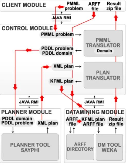
Figures 1 and 2 show the PDM architecture and the main algorithm of the implemented system, respectively. There are four main modules; each one can be hosted in a different computer connected through a network:Client,Control,Dataminingand Planner. We have used the Java RMI (Remote Method Invocation) technology that enables communication between different servers running JVM’s (Java Virtual Machine). The planner incorporated in the architecture is sayphi(De la Rosa, et al. 2007) and the DM Tool is WEKA (Witten & Frank 2005).

Figure 1 Overview of the PDM architecture.

DM-Request(pmml-file,domain):result pmml-file: PMML file with the DM task

domain: PDDL domain

problem=PMML2PDDL(pmml-file)

plans=RMI-Planner(domain,problem)

kfml-files=Plan2KFML(plans)

result=RMI-DMTool(kfml-files) returnresult

Figure 2 Algorithm for executing a DM request. TheClientmodule offers an interface that provides access to all the application functionalities. It generates a PMML file from a high level description of the DM task specified by the user using the interface. Then, it sends the PMML description to theControlmodule.

The Control module interconnects all modules and performs the required translations. The translations needed are: from PMML to PDDL, PMML2PDDL; and from a PDDL plan to KFML,

Plan2KFML. The input to the module is the DM task together with the dataset. Figure 2 shows the main algorithm. First, the PMML2PDDLtranslator generates the PDDL problem file from the PMML file. Then, the planner is executed to solve the translated problem. The returned set of plans is translated to several KFML files. Finally, the DM Tool is executed to process and run the translated KFML files.

TheDataminingmodule permits the execution of DM tasks in the WEKA DM Tool through Knowledge Flow plans. It obtains the model output and the statistics generated by the Knowledge Flow execution. This module also contains an Arff directory for managing the storage of the datasets that are necessary for the WEKA executions. The input to the module is a KFML file and the output is a compressed file. Some other DM Tool could be used instead of WEKA. Then, we would only have to adapt the translator of plans, to deal with the input requirements of the new tool.

ThePlanningmodule receives each problem and domain in PDDL format. It returns a set of plans in XML format ready for the conversion to a KFML format. Currently, planning tasks are solved by the_sayphiplanner (De la Rosa et al. 2007), but the architecture could potentially use any other planner that supports fluents, conditional effects and metrics. We have used _sayphi because it: i) supports an extensive subset of PDDL; and ii) incorporates several search algorithms

(5)

able to deal with quality metrics, and generate several plans. One of the limitations we have on choosing planners is that currently state-of-the-art planners cannot handle cost metrics that depend on the state, though defined within PDDL.1

4 Modelling DM Tasks in PDDL

The main challenge of our approach is how to model DM tasks by means of AP. As we said, an AP task is defined by two files, the domain definition and the problem description, whereas the DM task is defined by the PMML file. This section describes the contents of each of these three files for automatically compiling DM tasks into planning tasks.

4.1 The PMML file

The PMML file distributes the information the planning problem requires along all its parts. The only section that is not used is the mining build task, that will be generated after the model is built. The header of the PMML file contains the following information:

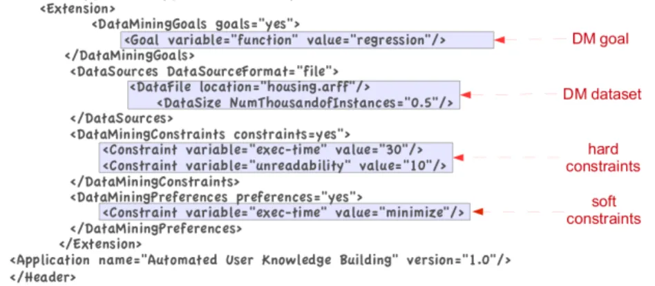
• The DM goal. It can be classification, regression or clustering.

• The dataset location and size.

• The hard and soft constraints of the user. An example of hard constraint is obtaining an error lower than a given threshold, whereas minimizing the total execution time is an example of soft constraint or preference. We handle preferences and hard constraints over: i) exec-time, for minimizing/constraining the execution time, ii) percentage-incorrect, for minimiz-ing/constraining the classification error; iii)mean-absolute-error, for minimizing/constraining the mean absolute error in regression tasks and clustering, and iv) unreadability, for maximizing the understandability of the learned model (we transform maximizing the understandability of the learned model into minimizing/constrainingunreadability).

Figure 3 shows an example of the PMML header for defining a regression (goal) DM task where the execution time must be lower than 30, the unreadability lower than 10 (hard constraints) and the DM metric (soft constraint or preference) is minimizing the execution time.

Figure 3 Example of the header part of a PMML file defining a DM task.

The data dictionary includes one field for each attribute in the dataset. For example: <DataDictionary numberOfFields="14">

...

1

(6)

The transformation dictionary includes one function for each possible filter the user wants to apply over the input data. For example:

</Extension>

</TransformationDictionary>

Finally, the model part contains the definition of the DM models. For example: <TreeModel modelName="treemodel2" functionName="regression" algorithmName="M5">

</Extension>

<MiningSchema> <MiningField name="housing"/> </MiningSchema> ...

</TreeModel> ...

The user can specify the same model but with different parameters. In this case, there must be two entry models with different modelName and the model parameters are encoded in the

Extension part. In general, for most DM tasks, the user would include in the PMML file the full set of WEKA DM techniques and some common settings for their parameters. This is easily done through the user interface in the Client module.

4.2 The PDDL Domain File

The PDDL domain file contains the description of all the possible DM tasks (transformations, training, test, visualization, . . . ). Each DM task is represented as a domain action. The PDDL problem files contain information for a specific dataset (i.e. dataset schema, the suitable transformation for the dataset, the planning goals, the user-defined metric, etc.). Domain predicates define the state space containing static information (i.e. possible transformations, available training or evaluation tasks, etc.) and dynamic information that changes during the execution of all DM tasks (e.g. adding the fact that the dataset has already been pre-processed or evaluated). The functions allow us to define thresholds for different kinds of DM features (e.g. error, execution time threshold, or understandability of a model) and to store the values updated during the execution (e.g. total estimated error, execution time, or understandability).

There are different kinds of actions in the domain file:

• Preparation Actions for specific manipulations of the dataset. For instance, load-dataset or datasetPreparation for splitting the dataset or preparing it for cross-validation after finishing the data transformation. Preconditions verify the dataset and test mode availability with the predicates available and can-learn, respectively. Figure 4(a) shows the PDDL datasetPreparationaction. It adds the effect(eval-on)for allowing the training and testing. We use functions to record estimates of the execution time of actions. The values of these functions are expressed in the problem definition. We assume the execution time is proportional to the number of instances (in fact, thousands of instances) and depends on the test mode. For example, we estimate that the preparation factor for splitting is 0.001 and for cross-validation is 0.005. The (loaded ?d)precondition is an effect of the load-dataset action.

• Transformation Actions represent the transformations or filters that can be applied to the dataset. They are defined as apply-transformation-<filter> actions. Preconditions verify

(7)

(a) (:action datasetPreparation (b)(:action apply-transformation-AttributeSelection :parameters (?d - DataSet ?t - TestMode) :parameters (?d - DataSet ?i - TransfInstance) :precondition (and (loaded ?d) :precondition (and (pre-process-on ?d)

(can-learn ?d ?t)) (known-fields ?d)

:effect (and (eval-on ?d ?t) (transformation ?i AttributeSelection)) (not (pre-process-on ?d)) :effect (and (applied-instance ?d ?i)

(not (loaded ?d)) (applied-transformation ?d AttributeSelection) (increase (exec-time) (not (known-fields ?d))

(* (thousandsofInstances) (increase (exec-time)

(preparationFactor ?t))))) (* (* (filter-time AttributeSelection) (thousandsofInstances)) (* (dataDictionaryNumberOfFields)

(dataDictionaryNumberOfFields)))))

(c) (:action train-classification

:parameters (?mi - ModelInstance ?m - Model ?n - ModelName ?d - DataSet ?fi - FieldName ?t - TestMode) :precondition (and (learnable ?mi)(is-model ?mi ?m) (implements ?m classification ?n)(is-field ?fi ?d)

(dataDictionaryDataField-otype ?fi categorical)(eval-on ?d ?t)) :effect (and (is-classification-model ?mi ?d ?fi) (has-model-of classification)

(not (pre-process-on ?d))(not (learnable ?mi)) (increase (unreadability) (model-unreadability ?m))

(increase (percentage-incorrect)(model-percentage-incorrect ?m)) (increase (exec-time) (* (* (model-exec-time ?m)(thousandsofInstances))

(* (dataDictionaryNumberOfFields)(dataDictionaryNumberOfFields))))))

Figure 4 Example of three actions in the PDDL domain.

the field type constraints and whether the filter has been included as a DM task for the dataset or not. The action usually adds a fact indicating that the task has been done (e.g. the normalize transformation adds to the state the fact (normalized DataSet)). Figure 4(b) shows the attribute selection PDDL action, that includes several predicates(known-fields), (transformation ?i AttributeSelection) and (pre-process-on ?d) to check respectively if the attributes are known at planning time, if the filter has been included in the PMML file, and if the planner is still at the pre-process phase.

• Training Actions, i.e. the operations for training models with datasets. They are described in the form oftrain-<model-type>, where<model-type>can beclassification, regressionor clustering. In each type, the action parameters indicate different models previously defined in the PMML file. There is a precondition for verifying if the model instance is learnable

and another one to verify the model. These actions add the fact that the selected option is a model for the dataset with the predicateis-<model-type>-model. Figure 4(c) shows the PDDL action for a classification task. Training tasks always increase errors (in case of classification they represent classification error,percentage-incorrect), and the unreadability of the learned model.

• Testing Actions evaluate models. They are defined in the form oftest-<model-type>. These actions usually follow their corresponding training action. Examples are cross-validation or split.

• Visualizing and Saving Actions generate the output of the learning process. They are described in the form ofvisualize-<result-option>.

A typical plan contains the following actions. load-dataset is the first action in every plan. Then, the plans can contain zero or more transformation actionsapply-transformation-x. In the current version, after the attribute selection filter is applied, no other filter is allowed. The reason is that this filter eliminates attributes, and it is impossiblea priorito predict which attributes will be eliminated. Therefore, we can not apply more filters, since we do not know which attributes will be available in the dataset after the application of the attribute selection filter. We plan to remove this constraint by interleaving planning and execution as explained later. The following action is thedatasetPreparationthat prepares the dataset for splitting or for a cross-validation. Then, there are three alternative actions for training,train-classification, train-regression and train-clustering, another three for testing, test-classification, test-regression and test-clustering, and three more for visualizing the model visualize-classification-model,

(8)

visualize-regression-modelandvisualize-clustering-model. The last action in all plans is the visualize-resultthat outputs the learning results (errors, execution time, . . . ).

Information in the problem file is automatically obtained from the PMML file using the translator described in the next section. This information, specific to a dataset, is used by the planner to instantiate all the possible actions specified in the PMML file by the user and to handle constraints imposed to the planning task.

4.3 Compilation of a PMML into a PDDL Problem

The PMML2PDDL translator automatically converts parts of a PMML file with the DM task information into a PDDL problem file. The problem file together with a domain file, that is fixed for all the DM tasks, are the inputs to the planner. The problem file contains the particular data for each DM episode, including the dataset description, the transformations and models available for that problem, and the possible preferences and constraints of the user.

A PDDL problem file is composed of four sections: the objects, the inits, the goals and the

metric.Inits(initial state of the problem), as explained below, is composed of some propositions common to all problems (static part of the problem specification) and others are translated from the PMML file (dynamic part). The Goals are currently fixed for all the problems, and consist of performing some learning action (extracted from the PMML file), followed by visualizing the result (saving the statistics required to analyze the generated DM models). TheMetricsrepresent the formula whose value will be minimized, i.e. the soft constraints or preferences defined in the header of the PMML file. So far, the translator always deals with the optimization of a single criterion. However, it can be easily extended to handle any linear function of two or more criteria. The hard constraints are encoded by adding numerical goals to the PDDL problem. For example, we might have: (<= (exect-time) 30)or (<= (unreadability) 10).

The static part of the initial-state specification includes all the propositions concerning the predicates is-model, learnable, allow-visualization, available and can-learn, explained in the previous section, and the initial values of the counter functions. We abstract the meaning of the constraints by defining a counter function for each learning model and constraint type. For ex-ample, thetreemodel2defined above requires three counters:(model-unreadability treemodel2), (model-mean-absolute-error treemodel2) and (model-exec-time treemodel2). The training ac-tion increases the corresponding funcac-tions, i.e. (unreadability), (mean-absolute-error) and (exec-time) for regression tasks, with the corresponding counter-function value. These values can be seen as weights assigned to learning models. They have been estimated by an expert although, in the next future, they will be learned applying machine learning algorithms.

The dynamic part includes the information about the dataset, the hard constraints and preferences, the transformations and the models available for the DM request. The standard PMML is flexible enough to contain all the information required to automatically compile DM tasks into planning tasks. For instance, Figure 3 describes how the user preferences and constraints, as well as many other data mining knowledge, are included in the PMML as extensions of the standard language. Once all the extensions are defined, the translation process is simple: the complexity relies on defining such extensions, i.e. defining the relationships between the data mining objectives and the planning concepts.

5 Planning for DM Tasks

As we mentioned in the previous section, sayphi solves the planning task depending on the metric specified in the PMML file._sayphiincludes a collection of search algorithms and domain-independent heuristics. Here, we use a Best-first Search that, once it finds a solution, continues exploring nodes in order to find multiple solutions. It is likely that the user and the planner will not agree about which are the best plans, because the planner’s cost estimates (execution time, accuracy, understandability, etc.) are not very accurate. Therefore, diversity is the only way to

(9)

avoid this problem. Figure 5 shows a simple example (without transformation actions) of a best-cost solution plan when the translated PDDL indicates the error as the problem metric. Likewise, Figure 6 shows a best-cost solution plan for the same problem, but using the metric of minimizing execution time. In the first plan aNeural Networkis preferred in thetrain-classificationaction because it has a lower estimated error than applying the same action with another model. The second plan has two differences. The Split parameter is selected instead of Cross-validation, and Tree Model is preferred instead of Neural Network because these actions are cheaper in terms of execution time. The best-cost solution using the unreadability metric coincides with the second plan, since the Tree Model is the action that minimizes the estimated cost (inverse of understandability) for the training action.

0: (LOAD-DATASET INITIALDATASET)

1: (DATASETPREPARATION INITIALDATASET CROSS-VALIDATION) 2: (TRAIN-CLASSIFICATION NN NEURALNETWORK

NNMODEL4 INITIALDATASET CLASS CROSS-VALIDATION) 3: (TEST-CLASSIFICATION NN INITIALDATASET NEURALNETWORK

CLASS CROSS-VALIDATION RESU)

4: (VISUALIZE-RESULT NN INITIALDATASET CROSS-VALIDATION RESU TEXT)

Figure 5 An example of plan minimizing the error.

1: (DATASETPREPARATION INITIALDATASET SPLIT) 2: (TRAIN-CLASSIFICATION TREE TREEMODEL

TREEMODEL1 INITIALDATASET CLASS SPLIT) 3: (TEST-CLASSIFICATION TREE INITIALDATASET

TREEMODEL CLASS SPLIT RESU) 4: (VISUALIZE-RESULT TREE INITIALDATASET

SPLIT RESU TEXT)

Figure 6 An example of plan minimizing the execution time.

Most of the action costs rely on formulae that take into account the number of instances, the number of attributes and pre-defined weights for each parameter (e.g. a constant function defined in the initial state), such as(= (model-percentage-incorrect NeuralNetwork) 5). These constant values were set by a DM expert in order to reproduce estimated common results. Accordingly, the total cost for a solution is taken as an estimate, since the real cost in this application can not be known in advance. One solution consists of allowing sensing actions: sensing the environment after each action execution could establish real costs, but we have not included this process at the current state of the project. Anyway, these estimations aim to guide the search process toward the most promising solutions. The DM Tool will compute them later on.

6 Obtaining DM Models

The Planner module outputs all the generated plans encoded in an XML file.Plan2KFMLtranslates each plan into a KFML file, so it can be executed by the WEKA Knowledge Flow. Figure 7 shows a plan (in a standard format, not XML) generated by_sayphi. The translator generates as output a new KFML file with an equivalent plan plus some new actions that the WEKA Knowledge Flow can execute. Each action in the PDDL domain corresponds to one or many WEKA components. Therefore, the translator writes for each action in the plan the corresponding set of XML tags that represent the WEKA component. For instance, Figure 8 shows a section of the KFML file generated from the plan in Figure 7. This part corresponds to the third action in the plan, i.e., theDATAPREPARATIONaction.

Actions appearing in a plan can correspond to one of these cases:

• The action corresponds to exactly one WEKA component. For instance, the LOAD-DATASET action corresponds to the ArffLoader component of the knowledge flow. Some additional information may be needed from the PMML file (e.g., the URI of the dataset to be loaded).

• The action corresponds to many WEKA components and the action parameters decide which component needs to be selected. For instance, in the DATASETPREPARATION action, the second parameter indicates the type of operation. Thus,CROSS-VALIDATIONcorresponds to the CrossValidationFoldMaker component in the knowledge flow, andSPLIT corresponds to the TrainTestSplitMaker component.

• The action corresponds to many WEKA components and the action parameters only specify the name of a technique or model. In these cases, the translator needs to extract that

(10)

1: (APPLY-TRANSFORMATION-ATTRIBUTESELECTION INITIALDATASET ATTRIBUTESELECTION4)

2: (DATASETPREPARATION INITIALDATASET CROSS-VALIDATION) 3: (TRAIN-CLASSIFICATION TREE TREEMODEL TREEMODEL1

INITIALDATASET CLASS CROSS-VALIDATION) 4: (TEST-CLASSIFICATION TREE INITIALDATASET

INITIALDATASET CLASS CROSS-VALIDATION RESULT) 5: (VISUALIZE-CLASSIFICATION-MODEL TREE

TREEMODEL GRAPH INITIALDATASET CLASS) 6: (VISUALIZE-RESULT TREE INITIALDATASET

CROSS-VALIDATION RESULT TEXT)

Figure 7 An example of a plan generated by

sayphi.

...

name="custom_name">CrossValidationFoldMaker</object> <object class="weka.gui.beans.CrossValidationFoldMaker"

name="bean">

</object> ...

Figure 8 A part of the KFML file corresponding to theDATASETPREPARATIONaction in the solution plan presented in Figure 7.

information from the PMML file in order to decide which KFML components should be selected. The information extracted from the PMML file includes the name of the component and the parameters that has to be written in the XML code. For instance, the TREEMODEL parameter of the TRAIN-CLASSIFICATION action corresponds to the J48 algorithm and some other component properties defined in the PMML file.

After writing all the components into the KFML file, the translator connects them in the order specified by the plan using the linking primitives of KFML. Finally, the translator adds some extra components in order to save the information generated during the execution. That information is composed of the learned models and statistical information as the execution time or the accuracy. The output files generated during the KFML executions (the model instance and the statistical information, for each input plan) are compressed together with the PDDL problem and the XML plans. This compressed file is returned to the user.

7 Experimental Results

In this section we present the experimental evaluation performed to test the PDM architecture. This evaluation has two purposes. On one hand, we want to illustrate the functionality of the architecture, testing the whole process for a variety of datasets. On the other hand, we want to verify the utility of ranking different knowledge flows based on the execution-time metric. In our case, a knowledge flow ranking is a list of plans sorted by the extimated execution-time. Building rankings allows us to compare estimated execution times calculated by the planner against real execution times spent by WEKA. A good ranking is an ordered list of plans where the ones that need less time to execute appear in the first positions of the list. This section is structured as follows: we first describe the experimental settings, then we explain how we evaluate knowledge flows rankings, and finally we present the obtained results.

7.1 Experimental Setting

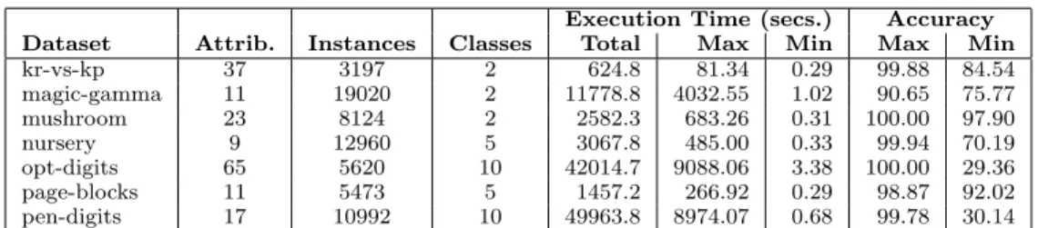
We have used seven datasets from the UCI KDD Archive 2_{. For each dataset we built a PMML} file with two filters (attribute selection and discretization) and six classification algorithms (J48, IBK, Simple-Logistics, Multi-layer Perceptron, RBF-Network and SMO). We keep WEKA default parameters for both filters and algorithms. In addition, the PDDL domain considers three evaluation methods: training-dataset, split and cross-validation, also with WEKA default parameters. As a result of different combinations, we got 72 different knowledge flows for each dataset. Table 7.1 presents the collected information for each dataset. The total time adds the time for executing all knowledge flows. Maximum and minimum values illustrate the variability for execution time and classification accuracy that can be observed when using a diversity of DM

2

(11)

processes and combinations. Even if we used a few alternatives from the point of view of DM, a huge variability can be observed, and justifies that when one has limited resources (time to perform the DM process, for instance) automatically generating those plans according to a given metric can be of a great help. For the set of possible plans/knowledge-flows the planner returns a list of plans ordered by the plan cost, computed using the metric. The positions in this ordered list serves as the ranking for the set of knowledge flows.

Execution Time (secs.) Accuracy

Dataset Attrib. Instances Classes Total Max Min Max Min

kr-vs-kp 37 3197 2 624.8 81.34 0.29 99.88 84.54 magic-gamma 11 19020 2 11778.8 4032.55 1.02 90.65 75.77 mushroom 23 8124 2 2582.3 683.26 0.31 100.00 97.90 nursery 9 12960 5 3067.8 485.00 0.33 99.94 70.19 opt-digits 65 5620 10 42014.7 9088.06 3.38 100.00 29.36 page-blocks 11 5473 5 1457.2 266.92 0.29 98.87 92.02 pen-digits 17 10992 10 49963.8 8974.07 0.68 99.78 30.14

Table 1 Collected data for the evaluated datasets. For the execution time, Total is the total time for executing all the knowledge flows obtained by PDM; Maximumand Minimum values are also given. The maximum and the minimum classification accuracy obtained by WEKA are shown in the last columns of the table.

In order to perform the rankings evaluation we set up PDM for the following configurations:

• Baseline Configuration: The PDDL files define different values for the fluents that weight the estimated execution time in filters and evaluation modes, but not for the learning algorithms. Therefore, all learning algorithms are supposed to take the same time to perform a learning and/or evaluation process over the same dataset. This represents the lack of knowledge about the learning and/or evaluation duration of the different algorithms.

• Average Configuration: The PDDL files also define different values for the fluents that weight the estimated execution time in the learning algorithms. More specifically, we estimate the fluent exec-time for each learning algorithm (see the effects of the train-classification

action defined in Figure 4(c)). This represents an improvement over the expert knowledge given to the planner, and assumes that a learning and/or evaluation process will take different time depending on the classification algorithm.

For obtaining the estimations of the execution time of the different learning algorithms in theAverage Configuration, we have taken the following three steps. (1) we have executed PDM with five smaller datasets from the UCI KDD Archive (i.e., Car, Credit-a, Habermann, Yeast and Hypothyroid), using all the learning algorithms. (2) For each algorithm, we computed its execution time as an average of the execution time in all datasets (this is the reason why this configuration is calledAverage Configuration). (3) This average is used to set the specific fluents of each algorithm in the problem file.

7.2 Evaluation Metrics for Rankings

For the ranking evaluation, the set of plans are also ordered by the real execution time, and the new position in the list reveals the right position that each plan should have. Suppose we denote asestimated(π) the position for the plan π in the plan list ordered by estimated time, and real(π) the position in the list order by execution time. For any two plans πi and πj, if estimated(πi)<estimated(πj) we consider an order switch wheneverreal(πi)>real(πj). In order to

compare both configurations we compute the following measures as done in (Rosset, et al. 2007):

• Single ranking order switches (∆): It counts how many pairs (πi, πj) in the plan list of

estimated times are ordered incorrectly when compared to real times.

• Weighted ranking order switches (W∆): It multiplies each incorrectly ordered pair by the ranking distance as a measure of the error being committed.

(12)

Then, these measures are normalized in the interval [0,1], where 0 represents the perfect reverse ranking (all possible ordering errors) and 1 corresponds to the perfect ranking (no ordering errors). The value of 0.5 corresponds to a ranking where plans are sorted randomly.

7.3 Results

Table 2 shows the two ranking measures for the evaluated datasets. We can observe that all values for both rankings are better than selecting plans randomly. This is mainly due to the high influence that the evaluation methods have in the total execution time. For instance, if one uses the same algorithm, it is expected that a 10-fold cross-validation will last longer than a single training with a dataset split. Values for the average configuration improved their corresponding value compared to the baseline configuration in five of the seven datasets, including the two datasets that last longer in the execution of all plans. This reveals the importance of having a good domain knowledge in the PDDL construction for obtaining good estimations. In the cases where the average configuration is worse, (kr-vs-kp and magic-gamma) we observed that most of the ordering errors were caused by some specific plans.In those plans, applying RBFNetworks was faster than applying SMO and IBK. This is not what normally happens neither in the five smaller sets used for computing the average values nor in the rest of the evaluated datasets.

Baseline Configuration Average Configuration

Dataset ∆ W∆ ∆ W∆ kr-vs-kp 0.612 0.665 0.606 0.649 magic-gamma 0.616 0.664 0.553 0.573 mushroom 0.585 0.622 0.613 0.658 nursery 0.626 0.677 0.684 0.752 opt-digits 0.601 0.646 0.758 0.855 page-blocks 0.632 0.689 0.686 0.761 pen-digits 0.577 0.617 0.777 0.866

Table 2 Measures for ranking order switches between estimated and real execution time in the evaluated datasets.

Despite the improvements obtained by the average configuration, there is considerable room for ranking refinements. First, extra knowledge can be integrated into the PDDL domain and problem, making cost functions depend on other variables (i.e. number of discrete/continuous attributes, the number of classes, statistics over a subset of instances, etc.). Second, estimated costs for DM tasks can be updated by a learning process that uses the execution (real) costs of tasks. Thus, a regression model, rather than an average, can give more accurate values. This is part of our current research agenda.

8 Related Work

In the recent years there is a growing interest on how Automated Planning can support DM. A first example, _inlen (Michalski & Kaufman 1998) can automatically pursue different DM tasks according to a high-level plan. However, it is the user who defines the plan. Other systems, like_aide (Amant & Cohen 1997), use a different planning approach closer to reaction: they continuously interact with the user suggesting the next action to be performed. That work presents three features that are interesting for this kind of tools, that we would like to explore in the future. First, they build upon a plan library (as other systems do (Morik & Scholz 2003, Bernstein et al. 2005)). Second, they use a hierarchical approach to planning as also used in (Engels 1996) (higher level tasks, such as pre-processing data, can be decomposed into lower level tasks, such as normalization followed by attribute selection). Third, they use a mixed-initiative reactive approach that interleaves planning and execution. In our case, we could devise such a scheme by extensively using interaction through the tool’s GUI, suggesting the next step to be performed, and executing it if the user so demands.

(13)

Opposite to the works that use hierarchical planning, we have preferred to use a more standard language as PDDL (hierarchical planners cannot use PDDL directly), given the existence of multiple planning systems using PDDL. Also, hierarchical planning requires defining the decompositions, which is not trivial due to the high interaction among the different components of the DM process. For instance, learning a neural network usually requires that the input data is normalized, while decision tree learning does not require that normalization process; but the result of the normalization process may be influenced by a previous instance selection process (for instance, if we eliminate out-layers). Therefore, the order in which both transformations occurs can be relevant to the result of the ML process. At the same time, that instance selection process could be required by a learning algorithm with a learning time that grows exponentially with the number of instances. Therefore, transformation functions constraint the learning algorithms that can be applied, and learning algorithms may force to apply some transformations in order to satisfy some user preferences (like learning time). Such strong interactions difficult the definition of knowledge-based decompositions, since the influence among different tasks are very high and unknown a priori.

ida(Bernstein et al. 2005) uses an ontology to describe the knowledge on tasks, subtasks, and primitive actions. This would be similar to the use of a hierarchical planner. An interesting idea in this work is the dynamic generation of a ranking of solutions (plans in our case), as we currently do. However, as other authors claim, obtaining multiple solutions can be costly, so we would like to interleave generation of multiple solutions with execution of previously generated solutions, as our tool can be distributed in several machines. Other works, as (Chien & Mortensen 1996), also use hierarchical planning techniques, but they focus on a very specific area of image processing for planetary science applications, where to build the hierarchy “ad-hoc” is easier. Pure Machine Learning approaches try to predict the most accurate algorithms to use taking into account the dataset characteristics like the number of attributes, noise level, standard deviations for the class distributions, etc. as derived from different studies, like the Statlog Project (Michie, et al. 1994). DM Tools can be characterized by the amount of human interaction with the discovery process required and/or supported (Goebel & Gruenwald 1999), and this interaction can be described as Autonomous, Human guided or Highly Interactive. The interesting point of the PDM architecture is that it permits different degrees of this interaction. For instance, when a DM plan is generated, the decision on whether to execute it or to generate a different plan could be delegated to the user. Active DM (Sumathi & Sivanandam 2006) is a related area where data is continuously mined at a desired frequency. As rules are discovered, they are added to a rule base, and if they already exist, the history of the statistical parameter associated with the rules is updated. The tasks to perform in a DM Process can also be extracted from an agenda of tasks prioritized by their plausibility (Livingston, et al. 2001). Plausibility can be calculated using a function of strengths of reasons given for performing a task and estimates of the interestingness of the items the task operates upon. However, all these methods are very dependent on the task or DM tool used.

The problem of planning for data modelling can be seen as an instance of the more general class of planning for softbots. For example, the Puccini system is a program for generating and executing plans in the presence of incomplete information (Golden 1997). In fact, it can be considered a domain specific system, because the knowledge representation formalism, the actions representation formalisms, and the planning module were designed having in mind the specific application to build, i.e. an Internet softbot for the UNIX operating system (Etzioni & Weld 1994). Opposite to that approach, the PDM architecture is designed assuming independent modules that use standard languages to communicate knowledge among themselves. Recent examples of the use of planning to create softbots are the composition of Web services (Hoffmann, et al. 2009), or business workflows (Rodr´ıguez-Moreno, et al. 2007), which also follow the PDDL framework, or the composition of data workflows (Ambite & Kapoor 2007), where a domain dependent planning algorithm performs a regression search in plan space in the same fashion as partial-order

(14)

planners such as UCPOP (Penberthy & Weld 1992). Those examples share similar challenges to the creation and execution of data mining workflows.

Recently, new efforts have appeared in the application of automated planning for DM. An example is the e-LICO project (An e-Laboratory for Interdisciplinary Collaborative Research in Data Mining and Data-Intensive Sciences, http://www.e-lico.eu/) which uses two different layers, the application and the DM layers, to separate domain specific knowledge from domain independent DM tools. A first step of this project builds a DM ontology, formalizing the key components that together compose an algorithm’s inductive bias. Based on this ontology, a meta-learner could infer algorithm selection guidelines by correlating an algorithm’s intrinsic bias with empirical evidence of its performance (Hilario, et al. 2009). Again, HTN (Hierarchical Task Network) is proposed to perform the planning task (Kietz et al. 2009), but no empirical results are shown yet. The use of ontologies to guide the composition of a KDD process is used in many works (Diamantini et al. 2009, Bernstein et al. 2005), but also with domain dependent planning systems. Another work (Zakova et al. 2008) introduces also the idea of using PDDL to describe the planning task, but up to our knowledge, without showing empirical results.

9 Conclusions and Future Work

This paper presents the PDM architecture for modelling DM tasks by using AP, based on an extensive use of standard representation languages. The contribution of the work is twofold: modelling the data mining task as an AP task and implementing an architecture with the appropriate translators able to compile any DM episode represented in the standard language PMML into the planning standard language PDDL. We have defined a PDDL domain that contains actions to represent all the possible DM tasks (e.g. transformations, training, test, or visualization). The domain is assumed to stay fixed for all the DM episodes, but each action contains preconditions that depend on the specific DM task to control its activation. The PDDL problems are automatically translated from a PMML file representing a DM episode adding the propositions for activating the allowed actions in the particular DM episode.

The practical benefits of the architecture are: i) providing a semi-automatization of the DM process allowing mixed-initiative in DM, ii) bridging the gap between DM and end-users, even if users have limited knowledge in DM (in the extreme, PDM allows a non-expert to use it as a black-box), iii) increasing the performance of DM (by analyzing the most probable interesting combinations), and iv) automatic configuration of the DM process. Also, the use of standard languages facilitates the replacement of the architecture modules for other techniques or tools that perform the same functionality. For example, we could exchange the planning or DM tool.

This model deals with plan metrics as minimizing the total execution time or the classification error. During the planning process, the metrics are computed from a planning point of view providing some estimated values for their increments caused by applying the actions. Their true value cannot be known until a DM Tool executes them, though. Thus, we plan to apply learning techniques to obtain more accurate estimations based on previous DM processes. Also, sensing the environment after each action execution could establish the real costs, which is also part of future work. Once the planner solves a problem, the solution plan is translated into a KFML file to be executed by the Knowledge Flow of WEKA.

Acknowledgements

This work has been partially supported by the Spanish MICINN under projects TIN2008-06701-C03-03, TRA-2009-008, the regional projects CCG08-UC3M/TIC-4141 and the Automated User Knowledge Building (AUKB) project funded by Ericsson Research Spain.

References

R. S. Amant & P. R. Cohen (1997). ‘Evaluation of a semi-autonomous assistant for exploratory data analysis’. InProc. of the First Intl. Conf. on Autonomous Agents, pp. 355–362. ACM Press.

(15)

J. L. Ambite & D. Kapoor (2007). ‘Automatically Composing Data Workflows with Relational Descriptions and Shim Services’. In The Semantic Web, vol. 4825 of Lecture Notes in Computer Science, pp. 15–29. Springer.

A. Bernstein, et al. (2005). ‘Towards Intelligent Assistance for a Data Mining Process: An Ontology Based Approach for Cost-Sensitive Classification’. IEEE Transactions on Knowledge and Data Engineering 17(4):503–518.

S. A. Chien & H. B. Mortensen (1996). ‘Automating Image Processing for Scientific Data Analysis of a Large Image Database’. IEEE Trans. Pattern Anal. Mach. Intell.18(8):854–859.

T. De la Rosa, et al. (2007). ‘Using Cases Utility for Heuristic Planning Improvement’. InCase-Based Reasoning Research and Development: Proceedings of the 7th International Conference on Case-Based Reasoning, pp. 137–148, Belfast, Northern Ireland, UK. Springer Verlag.

C. Diamantini, et al. (2009). ‘Ontology-Driven KDD Process Composition’. InAdvances in Intelligent Data Analysis VIII, vol. 5772 ofLecture Notes in Computer Science, pp. 285–296. Springer.

R. Engels (1996). ‘Planning Tasks for Knowledge Discovery in Databases; Performing Task-Oriented User-Guidance’. In Proc. of the 2nd Int. Conf. on KDD.

O. Etzioni & D. Weld (1994). ‘A softbot-based interface to the internet’. Communications of the ACM 37(7):72–76.

U. Fayyad, et al. (1996). ‘From data mining to knowledge discovery in databases’. AI Magazine17(3):37– 54.

F. Fern´andez, et al. (2009). ‘Assisting Data Mining through Automated Planning’. In P. Perner (ed.), Machine Learning and Data Mining 2009 (MLDM 2009), vol. 5632 of Lecture Notes in Artificial Intelligence, pp. 760–774. Springer-Verlag.

M. Fox & D. Long (2003). ‘PDDL2.1: An extension to PDDL for expressing temporal planning domains’. Journal of Artificial Intelligence Research pp. 61–124.

M. Ghallab, et al. (2004). Automated Planning - Theory and Practice. Morgan Kaufmann, San Francisco, CA 94111.

M. Goebel & L. Gruenwald (1999). ‘A Survey Of Data Mining And Knowledge Discovery Software Tools’. SIGKDD Explorations1:20–33.

K. Golden (1997). Planning and Knowledge Representations for Softbots. Ph.D. thesis, University of Washington.

M. Hilario, et al. (2009). ‘A Data Mining Ontology for Algorithm Selection and Meta-Learning’. In ECML/PKDD09 Workshop on Third Generation Data Mining: Towards Service-oriented Knowledge Discovery (SoKD-09), pp. 76–87.

J. Hoffmann, et al. (2009). ‘Message-Based Web Service Composition, Integrity Constraints, and Planning under Uncertainty: A New Connection’. Journal of Artificial Intelligence Research35:49– 117.

J.-U. Kietz, et al. (2009). ‘Towards Cooperative Planning of Data Mining Workflows’. In ECML/PKDD09 Workshop on Third Generation Data Mining: Towards Service-oriented Knowledge Discovery (SoKD-09), pp. 1–12.

G. R. Livingston, et al. (2001). ‘Closing the Loop: An Agenda- and Justification-Based Framework for Selecting the Next Discovery Task to Perform’. Data Mining, IEEE International Conference on 0:385.

R. S. Michalski & K. A. Kaufman (1998). ‘Discovery Planning: Multistrategy Learning in Data Mining’. InProceedings of the Fourth International Workshop on Multistrategy Learning, pp. 14–20.

D. Michie, et al. (eds.) (1994). Machine Learning, Neural and Statistical Classification. Ellis Horwood. K. Morik & M. Scholz (2003). ‘The MiningMart Approach to Knowledge Discovery in Databases’. In In Ning Zhong and Jiming Liu, editors, Intelligent Technologies for Information Analysis, pp. 47–65. Springer.

J. S. Penberthy & D. Weld (1992). ‘UCPOP: A sound, complete, partial order planner for ADL’. In Proceedings of the 3rd International Conference on Principles of Knowledge Representation and Reasoning.

M. D. Rodr´ıguez-Moreno, et al. (2007). ‘Integrating Planning and Scheduling in Workflow Domains’. Expert System with Applications33(2).

S. Rosset, et al. (2007). ‘Ranking-based Evaluation of Regression Models’. Knowledge and Information Systems12(3):331–353.

S. Sumathi & S. Sivanandam (2006). ‘Active Data Mining’. InStudies in Computational Intelligence (SCI), vol. 29. Springer-Verlag.

I. H. Witten & E. Frank (2005). Data Mining: Practical Machine Learning Tools and Techniques. 2nd Edition, Morgan Kaufmann.

M. Zakova, et al. (2008). ‘Planning for Data Mining Workflow Composition’. InSoKD: ECML/PKDD 2008 workshop on Third Generation Data Mining: Towards Service-oriented Knowledge Discovery.