submitted
to the
Combined Faculties for the Natural Sciences and for
Mathematics
of the
Ruperto-Carola University of Heidelberg, Germany
for the degree of
Doctor of Natural Sciences
put forward by
Diplom-Statistician: Annette Möller
Born in: Hamburg
In der jüngsten Vergangenheit wurde die Entwicklung von Wettervorhersagen über Ensemble Vor-hersagesysteme zum Standard in der Meteorologie. Vorhersage Ensembles werden generiert aus mehreren Durchläufen dynamischer Wettervorhersagemodelle, mit unterschiedlichen Anfangs- sowie Randbedingungen oder Parametrisierungen. Jedoch sind auch die Ensemble Vorhersagen nicht in der Lage, die Vorhersageunsicherheit der numerischen Wettermodelle vollständig zu erfassen. Deshalb weisen Ensembles oft Verzerrungen und Dispersionsfehler auf, sind also mangelhaft kalibriert. Um dieses Problem zu beheben wurden bereits erfolgreich statistische Methoden zur Nachbearbeitung von Ensemblevorhersagen entwickelt. Dennoch sind viele dieser etablierten Verfahren ausgelegt auf die Anwendung auf eine einzelne Wettervariable, an einem festen Ort und für einen festen Vorher-sagehorizont. Diese Arbeit präsentiert Erweiterungen der etablierten Nachbearbeitungsmethoden Bayesian model averaging (BMA) und Ensemble model output statistics (EMOS), mit dem Ziel Abhängigkeiten zwischen Wettervariablen sowie räumliche Abhängigkeiten zu erfassen, welche in den ursprünglichen Ensemblevorhersagen implizit vorhanden sind. Zu diesem Zweck wird eine Mehrschrittprozedur vorgeschlagen, welche sowohl für die Modellierung von Abhängigkeiten zwi-schen Wettervariablen als auch für die Modellierung räumlicher oder zeitlicher Abhängigkeitsstruk-turen geeignet ist. Diese Prozedur kombiniert ein univariates Nachbearbeitungsmodell wie BMA oder EMOS mit einer multivariaten Abhängigkeitsstruktur, z.B. mit Hilfe einer Korrelationsmatrix oder der multivariaten Rangstruktur des Vorhersageensembles. Eine auf BMA basierende multi-variate Nachbearbeitungsprozedur, welche die Abhängigkeit zwischen Wettervariablen modelliert, wird auf das 8-Mitglieder UWME Ensemble für den Nordwesten der USA angewendet. Das Ergeb-nis einer entsprechenden Fallstudie ist eine multivariate Vorhersageverteilung mit guter multivariater Kalibrierung und Schärfe. Eine räumliche Variante dieser multivariaten Nachbearbeitungsmethode basierend auf EMOS wird angewendet auf Temperatur Vorhersagen des 50 Mitglieder ECMWF En-sembles in Deutschland. Es wird eine räumlich adaptive Erweiterung von EMOS verwendet, welche von kürzlich entwickelten Methoden für eine schnelle und genaue Bayesianische Schätzung räum-licher Modelle profitieren kann. Die Prozedur führt zu guter univariater und multivariater Kalib-rierung und Schärfe. Außerdem können die räumlichen Strukturen der beobachteten Wetterfelder durch die Methode angemessen wiedergegeben werden. Beide hier betrachteten Erweiterungen ver-bessern Kalibrierung und Schärfe im Vergleich zum ursprünglichen Vorhersageensemble und zu etablierten univariaten Nachbearbeitungsverfahren.
In the recent past the state of the art in meteorology has been to produce weather forecasts from ensemble prediction systems. Forecast ensembles are generated from multiple runs of dynamical numerical weather prediction models, each with different initial and boundary conditions or param-eterizations of the model. However, ensemble forecasts are not able to catch the full uncertainty of numerical weather predictions and therefore often display biases and dispersion errors and thus are uncalibrated. To account for this problem, statistical postprocessing methods have been developed successfully. However, many state of the art methods are designed for a single weather quantity at a fixed location and for a fixed forecast horizon. This work introduces extensions of two estab-lished univariate postprocessing methods, Bayesian model averaging (BMA) and Ensemble model output statistics (EMOS) to recover inter-variable and spatial dependencies from the original ensem-ble forecasts. For this purpose, a multi-stage procedure is proposed that can be applied for modeling dependence structures between different weather quantities as well as modeling spatial or temporal dependencies. This multi-stage procedure combines the postprocessing of the margins by the applica-tion of a univariate method as BMA or EMOS with a multivariate dependence structure, for example via a correlation matrix or via the multivariate rank structure of the original ensemble. The multivari-ate postprocessing procedure that models inter-variable dependence employs the UWME 8-member forecast ensemble over the North West region of the US and the standard BMA method, resulting in predictive distributions with good multivariate calibration and sharpness. The spatial postprocessing procedure is applied to temperature forecasts of the ECMWF 50-member ensemble over Germany. The procedure employs a spatially adaptive extension of EMOS, utilizing recently proposed methods for fast and accurate Bayesian estimation in a spatial setting. It yields excellent spatial univariate and multivariate calibration and sharpness. Further the method is able to capture the spatial structure of observed weather fields. Both extensions improve calibration and sharpness in comparison to the raw ensemble and to the respective standard univariate postprocessing methods.
List of Figures . . . III
List of Tables . . . IV
Acknowledgments V
1 Introduction 1
2 Probabilistic Weather Forecasting 5
2.1 Postprocessing methods for ensemble forecasts . . . 7
2.1.1 Ensemble Model Output Statistics (EMOS) . . . 8
2.1.2 Bayesian Model Averaging (BMA) . . . 11
2.1.3 Geostatistical Output Perturbation Method (GOP) . . . 15
2.1.4 Spatial BMA . . . 17
2.1.5 Geostatistical Model Averaging (GMA) . . . 19
2.1.6 Ensemble Copula Coupling (ECC) . . . 21
2.2 Verification methods . . . 24
2.2.1 Calibration . . . 25
2.2.2 Sharpness . . . 29
2.2.3 Proper scoring rules . . . 30
3 Copulas 35 3.1 Notation and preliminaries . . . 35
3.2 Copulas and Sklar’s Theorem . . . 39
3.5 A Gaussian copula multi-stage procedure . . . 46
4 Multivariate extension of BMA 49 4.1 Combining BMA and Gaussian copulas . . . 50
4.2 Data . . . 55
4.3 Results . . . 56
4.3.1 Results at Sea-Tac Airport . . . 57
4.3.2 Aggregated results over the Northwest US . . . 61
4.4 Assessing statistical significance . . . 63
5 Spatially adaptive extension of EMOS 65 5.1 Gaussian fields and Gaussian Markov random fields . . . 66
5.2 Integrated Nested Laplace Approximation (INLA) . . . 71
5.3 The SPDE approach . . . 76
5.4 Markovian EMOS (MEMOS) . . . 83
5.5 Multivariate dependence structures . . . 90
5.6 Data . . . 93
5.7 Mesh configuration . . . 95
5.8 Training period . . . 97
5.9 Results . . . 99
5.9.1 Aggregated univariate results . . . 99
5.9.2 Univariate results at single stations . . . 104
5.9.3 Multivariate results . . . 109
5.9.4 Univariate results for composite quantities . . . 121
5.9.5 Samples from multivariate MEMOS versions . . . 125
6 Discussion 129
2.1 Different shapes of PIT histograms . . . 27
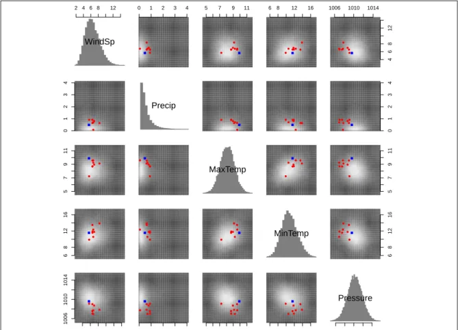
4.1 Estimated joint predictive distribution for January 1, 2008 at the observation station KSEA . . . 59
4.2 Multivariate rank histograms for the station KSEA . . . 60
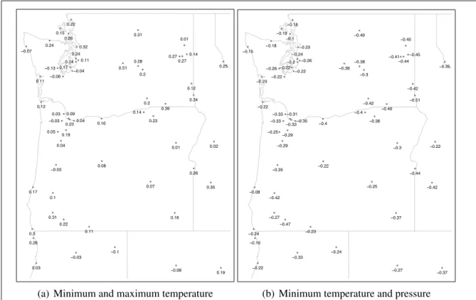
4.3 Estimated correlation at60observation stations in the Northwest US . . . . 62
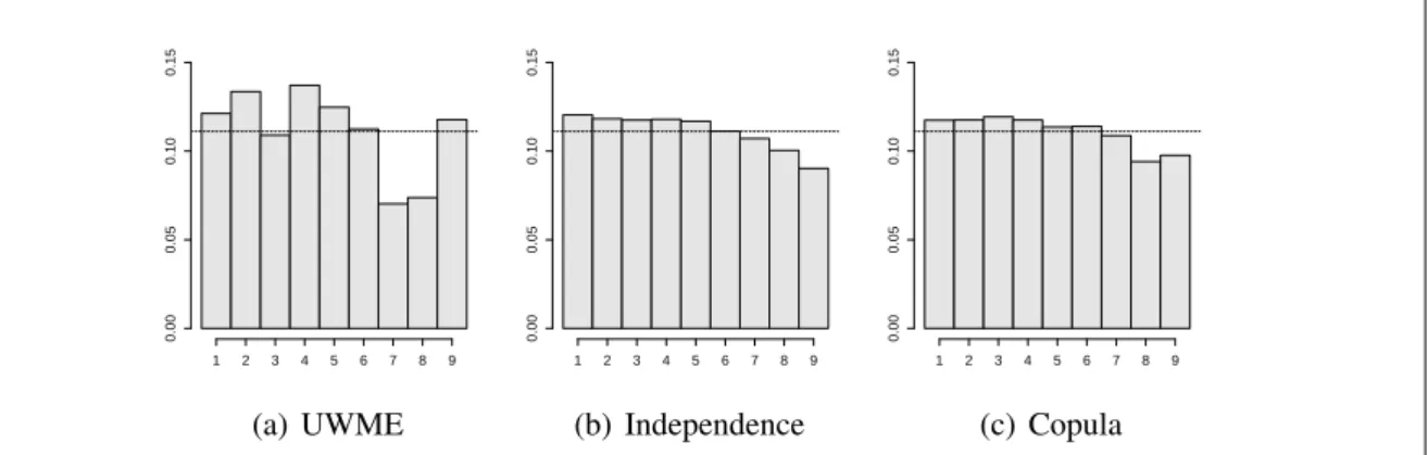
4.4 Multivariate rank histograms over all available observations at60stations in the Northwest US . . . 62
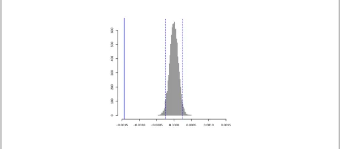
4.5 Permutation distribution of energy score differences . . . 64
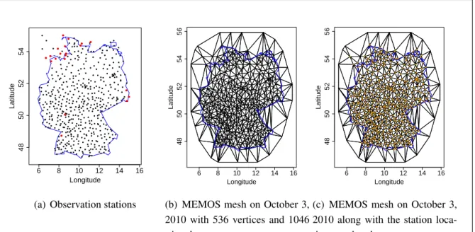
5.1 Station locations for temperature in Germany along with an example of a mesh used for MEMOS . . . 94
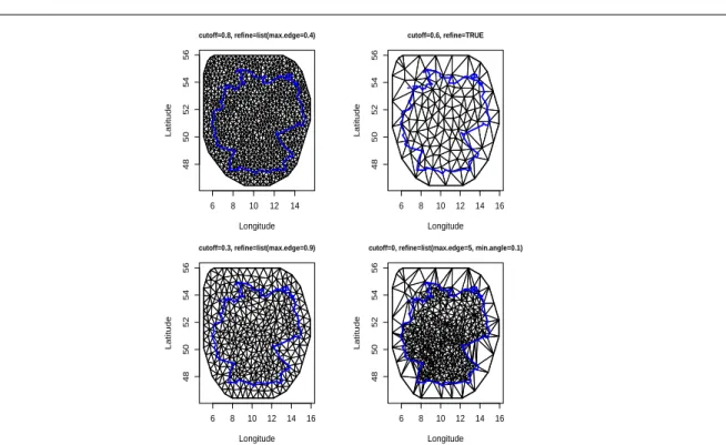
5.2 Mesh configurations with different parameters . . . 96
5.3 CRPS, MAE and RMSE for local EMOS and MEMOS plotted against length of training period . . . 99
5.4 Overall univariate calibration of MEMOS . . . 103
5.5 Univariate rank histograms for MEMOS at the station Borkum . . . 105
5.6 Univariate rank histograms for MEMOS at the station Frankfurt . . . 107
5.7 Univariate rank histograms for MEMOS at the station Baden-Baden . . . . 108
5.8 Multivariate rank histograms over four North Sea islands . . . 113
5.9 Multivariate rank histograms over eleven stations at the North Sea coastline 117 5.10 Multivariate rank histograms over three stations in East Germany . . . 120
5.11 Univariate rank histograms for minimum temperature over three stations in East Germany . . . 124
2.1 Ensemble BMA kernel functions for different weather variables . . . 14
4.1 Estimated correlation matrix at the station KSEA . . . 57 4.2 Multivariate predictive performance at the station KSEA . . . 60
4.3 Predictive performance averaged over60stations in the Northwest US . . . 63
5.1 Overall univariate predictive performance of MEMOS . . . 102
5.2 Univariate predictive performance of MEMOS at the station Borkum . . . . 104
5.3 Univariate predictive performance of MEMOS at the station Frankfurt . . . 106
5.4 Univariate predictive performance of MEMOS at the station Baden-Baden . 107
5.5 Pairwise distances in km between four North Sea islands . . . 110 5.6 Energy score over four North Sea islands . . . 112
5.7 Determinant sharpness over four North Sea islands . . . 112
5.8 Pairwise distances in km between eleven stations along the North Sea coastline114
5.9 Energy score over eleven stations along the North Sea coastline . . . 115
5.10 Determinant sharpness over eleven stations along the North Sea coastline . 116
5.11 Pairwise distances in km between three stations in East Germany . . . 118
5.12 Energy score over three cities in East Germany . . . 118
5.13 Determinant sharpness over three cities in East Germany . . . 119
5.14 CRPS for minimum temperature over three stations in East Germany . . . . 122
5.15 MAE for minimum temperature over three stations in East Germany . . . . 122
I gratefully acknowledge the financial support by the German Research Foundation (DFG) within the programme “Spatio-/Temporal Graphical Models and Applications in Image Ana-lysis” grant GRK 1653 and the scientific support by the Faculty of Mathematics and Com-puter Science of the University of Heidelberg.
Further, I would like to thank all the people that advised, supported and encouraged me during my PhD period. Specifically, I would like to acknowledge the assistance of my ad-visor Tilmann Gneiting, and of my mentors and coauthors Thordis Thorarinsdottir and Alex Lenkoski, providing very helpful discussions and ideas for developing the PhD project. Be-sides this I thank my colleagues Michael Scheuerer, Roman Schefzik and Kira Feldmann for helpful and inspiring discussions.
Apart from my scientific colleagues and advisors I would like to mention my friends Eva Didden and Anka George for uplifting me and cheering me up in times when I was suffering setbacks or having second thoughts. In particular I would like to thank my husband Jürgen for always backing me up, in scientific as well as as other concerns of real life.
Introduction
Analysis and prediction of current and future weather conditions has always been of great interest. In this day and age, an accurate forecast of weather becomes increasingly impor-tant in many economic and social areas, in the management of safe air and ship traffic, in agriculture and forestry, in efficient generation of energy with sustainable technologies as wind power and solar cells, or in civil protection in case of natural disasters such as floods, droughts, storms, forest fire and others. It is even of interest in the financial sector, for example considering the weather derivative.
During the past decades a change in the practice of weather prediction has been observed. Up to the beginning of the 1990s, weather prediction was a purely deterministic venture. National and international weather research centers run different sophisticated numerical weather prediction (NWP) models. The output of these models are deterministic point fore-casts for future weather conditions. However, deterministic point forefore-casts cannot address uncertainties such as imperfect model formulations or incorrect initial and boundary condi-tions used to run the model (Leutbecher and Palmer, 2008).
Numerical weather prediction models are still run today, but with a change towards the im-plementation of (dynamical) ensemble forecast methods. Ensembles of forecasts address prediction uncertainty and allow for probabilistic forecasting. A forecast ensemble is cre-ated by multiple runs of the numerical model, with a set of different initial conditions and lateral boundary conditions and/ or with different representations of the mathematical models used to describe the atmosphere. Dynamical ensembles can capture nonlinear uncertainties in forecasts, but they require considerable computational power.
However, ensemble forecasts still have their shortcomings. Often, ensembles exhibit sys-tematic biases as well as dispersion errors. The ensembles therefore lack calibration (Hamill and Colucci, 1997) and are typically underdispersed. To address these shortcomings several statistical methods of postprocessing the ensemble forecasts have been developed (Wilks and Hamill, 2007). Such methods correct for biases and dispersion errors in light of the principle ’maximizing sharpness subject to calibration’ proposed by Gneiting et al. (2007). An addi-tional advantage of statistical postprocessing is the fact that the postprocessing models yield full predictive probability distributions for the weather quantities of interest. In many appli-cations, the postprocessed ensemble outperforms the raw ensemble in terms of calibration and sharpness.
There are two main approaches of postprocessing, which are the basis for several extensions. The Ensemble Bayesian model averaging (BMA) proposed by Raftery et al. (2005) estimates the predictive density as a mixture of the individual densities associated with each ensemble member. The Ensemble model output statistics (EMOS) technique introduced in Gneiting et al. (2005) combines all ensemble forecasts in a multivariate regression approach. These methods, especially BMA, have been adapted in various ways to account for the character-istics of different weather quantities.
Many of the postprocessing techniques based on BMA and EMOS, however, are designed for a single weather quantity and a fixed location. They do not take into account dependencies between weather quantities or spatial dependencies between observation locations. For ex-ample for accurately forecasting composite quantities such as minima, maxima or averages, it is important to incorporate spatial structures and correlations among the location-specific forecast uncertainties.
Several approaches have already been developed on the basis of BMA or EMOS that account for spatial dependency structures in different ways. The main approaches are the Geostatis-tical model averaging (GMA) introduced by Kleiber et al. (2011a) and methods based on the Geostatistical output perturbation (GOP) method (Gel et al., 2004). While the first approach estimates spatially adaptive model parameters from all ensemble members, the second one aims at sampling spatially consistent and jointly calibrated samples of weather fields by em-ploying only a single ensemble member or point forecast.
This work contributes to the postprocessing literature in two ways. On the one hand, it intro-duces a new way of multivariate postprocessing where dependencies between weather quan-tities are incorporated in the predictive distribution by combining existing variants of BMA for different types of weather quantities with a multivariate dependence structure induced by a Gaussian copula. This method yields a joint predictive distribution for several weather
variate dependence structure. Nonetheless, a generalization to other types of dependence structures is straightforward and already utilized in the spatial approach discussed next. In the postprocessing literature multivariate postprocessing approaches are rarely found. Al-though Schoelzel and Friederichs (2008) consider the estimation of bivariate copulas to model the distribution of two weather quantities jointly (they apply this method to weather quantities as well as to other environmental variables), they are not employing these copula approaches in a context of ensemble postprocessing, only for observations of weather quan-tities. The work published by Möller et al. (2013) that is presented here, explicitly develops a multivariate ensemble postprocessing procedure to jointly model several weather quantities that closes a gap in the postprocessing literature.
On the other hand, this thesis develops a spatial postprocessing method by combining the advantages of GMA and GOP based methods. This postprocessing approach, called Marko-vian EMOS (MEMOS), extends the standard EMOS model to have spatially adaptive model parameters by assuming spatial Gaussian fields on them. The method additionally allows for producing samples from a spatial joint distribution by combining the basic MEMOS method with certain types of multivariate dependence structures in a multi-stage procedure. A fur-ther advantage is the possibility to utilize a recently developed methodology that allows to compute an explicit Gaussian Markov random field representation of a Gaussian field with Matérn covariance function (Lindgren et al., 2011). A direct link between the two types of random fields can be established via the solution of a stochastic partial differential equa-tion (SPDE). This methodology yields a considerable computaequa-tional benefit when estimating the parameters of the postprocessing model. The resulting postprocessing model was called Markovian EMOS to honor the specific markovian structure of the underlying GMRF repre-sentation.
The remainder of this work is organized as follows. Chapter 2 gives an overview on prob-abilistic weather forecasting in general as well as on several established univariate postpro-cessing methods. Chapters 4 and 5 present the multivariate and spatial extensions of the BMA and EMOS methods. For the spatial version the theory of Gaussian Fields, Gaussian Markov random fields and the link between both concepts via the solution of an SPDE is introduced. The respective chapters review the theory behind the developed methods and present the data employed for each of the approaches along with case studies analyzing their predictive performance.
In Chapter 3 some general theory about copulas is introduced, as Gaussian copula methods are employed in Chapter 4 to set up a multivariate dependence structure.
Chapter 6 briefly summarizes the key results of this work and discusses alternative ap-proaches as well as an outlook on future research plans extending the obtained methods in various directions.
Probabilistic Weather Forecasting
Current practise in predicting future weather is the use of numerical weather prediction (NWP) models. These are deterministic numerical simulation models representing the phy-sics of the atmosphere. The NWP models are based on several dynamical partial differential equations in different variables describing the evolution of the states of atmosphere. To obtain deterministic forecasts for future atmospheric states the involved equations are dis-cretized on a grid with a certain resolution (differing with the type of NWP model) and run forward in time. A set of initial and boundary conditions describing the current state of the atmosphere at time stept is assimilated from observations at time stept. The informa-tion is then used to run forward the NWP model in time and obtains predicinforma-tions of future atmospheric states at time stepst+l,l≥1.
There are different types of NWP models that are run operationally, among them global mod-els and mesoscale (limited-area) modmod-els. Different global modmod-els are run in real time all over the world, such as the European Centre for Medium-Range Weather Forecasts (ECMWF) model in Europe, the National Centers for Environmental Prediction (NCEP) model in the United States or the Meteorological Service of Canada (MSC) in Canada. Global models typically have a horizontal resolution of 36 - 100 km. The mesoscale models have a much higher resolution, typically about 2 - 36 km horizontally. They usually employ initial and boundary conditions provided by one or several global models.
An NWP model issues a single deterministic forecast and is therefore not capable of as-sessing the forecast uncertainty. However, there are major sources of uncertainty present in NWP models, such as an incomplete network of observations, measurement errors or in-correct model formulations due to incomplete knowledge of all physical processes in the
atmosphere.
The atmosphere is a chaotic system, very small perturbations of the current state can already lead to an increasingly large change in the evolution of the atmosphere so that after some time the development of the original state and the perturbed state are completely different (Lorenz, 1963). The chaotic nature of the atmosphere leads to significant forecast errors as minute errors in the initial conditions can grow exponentially during the integration process of the NWP model. This makes a single deterministic forecast useless when it comes to the assessment of the forecast uncertainty.
Ensemble methods are one manner of accounting for this problem. They lead to consider-able improvements in the forecast skill. This was explored elaborately for medium-range forecasts (2-10 days) (Toth and Kalnay, 1993; Molteni et al., 1996) and there is also research concerning the application of ensembles to short-range forecasts (0-48h) (Eckel and Mass, 2005; Hamill and Colucci, 1997).
Ensemble forecasting adopts the idea of predicting probabilities for future weather events (Leutbecher and Palmer, 2008). Pushing forward the ensemble forecasting in daily weather prediction lead to a change from purely deterministic weather forecasts to a more probabilis-tic approach. The idea of probabilisprobabilis-tic forecasting through ensemble forecasts is carried out by using a set of different initial and boundary conditions, all consistent with observations and observation errors, different model physics or model perturbations or even different nu-merical models. An ensemble of forecasts is then generated by running an NWP model with a varied set of initial conditions and/or perturbations or by employing a different unique nu-merical model for each run. There are several types of ensembles, according to the way their members are generated, see e.g. Eckel and Mass (2005):
Multi-analysis ensembles are produced by employing a single numerical model and run it multiple times, each time with a different set of initial conditions. Multi-model ensembles are obtained by employing a separate numerical model for each ensemble member, but run these multiple models with a single set of initial conditions. Multi-model multi-analysis ensembles are a combination of both types described above. Multiple numerical models are run, each with multiple sets of initial conditions, so each ensemble member is a specific combination of a certain numerical model with a certain set of initial conditions.
An example for a multi-analysis mesoscale ensemble system is the University of Washing-ton Mesoscale Ensemble (UWME), operating at lead times up to three days (Grimit and Mass, 2002; Eckel and Mass, 2005). It comprises of eight members that are obtained by using eight analyses from different operational forecast centers as initial conditions in the
fifth-generation Pennsylvania State University - National Center for Atmospheric Research Mesoscale Model (PSU-NCAR MM5). The PSU-NCAR MM5 model is succeeded by the WRF (Weather Research and Forecasting) model presently. In Section 4 some more infor-mation on the UWME ensemble is given, as the WRF UWME ensemble is employed in the case study for the multivariate postprocessing extension.
A forecast ensemble allows to combine the individual members for example by using the ensemble mean as a single deterministic forecast, as well as to estimate the forecast uncer-tainty by considering the ensemble variance or the root mean square error. On average, the ensemble mean outperforms each of the individual ensemble members (Grimit and Mass, 2002).
For a unimodal predictive distribution, variations in the width of the distribution from fore-cast to forefore-cast can be directly linked to the predictive skill of the mean forefore-cast. The spread of the ensemble measures the width of the predictive distribution and therefore provides a tool to assess the predictive skill of the ensemble mean. Specifically, Whitaker and Loughe (1998) found a positive correlation between the ensemble spread, which is known a priori, and the forecast errors, only known a posteriori. This phenomenon is called spread-error correlation or spread-skill relationship.
2.1
Postprocessing methods for ensemble forecasts
Ensembles allow for probabilistic forecasts of continuous weather variables, such as sea level pressure or surface temperature. Ideally, a probabilistic forecast takes the form of a predictive cumulative distribution function (CDF) or a predictive probability density func-tion (PDF). However, ensemble forecast systems are finite, they typically employ 5 up to 50 members. Hence, the raw ensemble output does not provide full predictive PDFs for continuous quantities, and some form of postprocessing is required.
Besides this, there are several additional challenges in the development of appropriate sta-tistical postprocessing methods. The current NWP systems typically show systematic biases (forecast errors) and the ensembles lack calibration, for details see Section 2.2.1, they are very often underdispersed (Hamill and Colucci, 1997), as the ensembles only capture some of the uncertainties of numerical weather forecasting (Raftery et al., 2005).
Many different postprocessing methods are available these days, most of them can be mod-ified to be suited for various weather quantities. There are two main approaches in the
existing postprocessing literature. The first type of methods is based on the ensemble BMA approach, where the predictive distribution is constructed as a mixture of individual kernel densities assigned to each forecast member. Each kernel density depends only on a specific forecast member. The weights of the mixture components are obtained from the predictive skill of the respective ensemble member. The second type of methods is based on the EMOS approach, where the predictive distribution is obtained via a multiple linear regression of the observations on all ensemble members.
These two basic postprocessing approaches have been extended and modified in various ways to account for the need of the applications to other than normally distributed weather quantities as well as for other requirements as taking into account dependency structures.
The following sections give an overview on the most important methods, that are frequently used, without any claim to be complete.
2.1.1
Ensemble Model Output Statistics (EMOS)
The ensemble model output statistics (EMOS) methodology was introduced by Gneiting et al. (2005). It addresses bias and dispersion errors of the raw forecast ensemble. The EMOS technique is motivated by the multiple linear regression model called model output statistics (MOS) in the context of applying linear regression equations to output of numerical weather prediction models (Glahn and Lowry, 1972; Klein and Glahn, 1974; Wilks, 2006, 2009). It has enjoyed popularity in the application to deterministic-style and probability of precipitation forecasts. The general idea of the MOS method is to combine the output of the numerical weather prediction models (numerical deterministic-style forecasts for different variables) with real observations made at observation stations to get improved forecasts at the considered stations. By taking into account the observations as well, the numerical forecasts can be verified or adapted to the situation at a specific station, after having interpolated the numerical forecast from the model grid to the respective station location. The regression model uses those parameters of the numerical model output that have an effect on a weather quantity of interest, like e.g. surface temperature or sea level pressure.
The EMOS technique is typically designed for the application to a univariate weather quan-tity, a fixed location and for a fixed forecast horizon. The basic method is not taking into account dependences with other weather quantities nor is it able to capture spatial or tem-poral dependencies. Specifically, let x1, . . . , xm denote a forecast ensemble of size m for a univariate quantity Y, where all individual forecast members are distinguishable. Using
the ensemble members as predictors in the multiple linear regression model this leads to the regression equation
Y =a+b1x1+. . .+bmxm+ε, (2.1)
wherea, b1, . . . , bm are regression coefficients and ε is an error term with varianceσ2 and mean 0.
Equation (2.1) is defined for each considered observation case i = 1, . . . , N and the error termsεi are assumed to be independent ofεi0 for alli6=i0. For convenience, the indexifor
the observations is omitted.
The model (2.1) can easily be adapted for indistinguishable forecast ensembles, as e.g. the ECMWF ensemble utilized in Chapter 5, by assuming all multiplicative bias-correction pa-rameters to be equal, that is,bk =b,k = 1, . . . , m.
Gneiting et al. (2005) propose this approach to improve the predictive performance of the ensemble with the additional benefit that the postprocessing method yields full predictive PDFs from a forecast ensemble for a continuous weather quantity. When assuming the error term to be normally distributed, that isε∼N(0, σ2), this leads to the following distribution of the quantityY given themensemble members:
Y|x1, . . . , xm ∼N a+ m X k=1 bkxk, σ2 . (2.2)
This conditional distribution allows to obtain estimated PDFs and CDFs from the regression Equation (2.1) in a straightforward way. The EMOS approach corrects for model biases and accounts for dispersion errors by performing a simple bias correction through the linear combination of the ensemble members with the bk as multiplicative coefficients and a as additive coefficient. However, with the assumption of a constant model variance the spread of the original ensemble is not taken into account in the model, and so it ignores the spread-skill relationship (Whitaker and Loughe, 1998; Barker, 1991). Gneiting et al. (2005) propose to model the variance of the error term as a linear function of the ensemble spread:
Var(ε) =c+dS2, whereS2is the ensemble variance andcanddare nonnegative coefficients.
In this case the predictive distribution of the quantityY given the ensemble members is given as Y|x1, . . . , xm ∼N a+ m X k=1 bkxk, c+dS2 (2.3)
In the above model formulation the regression parametersbk can be positive and negative. In applications positive as well as negative regression coefficients may occur. Negative
co-efficients are typically caused by collinearities of the ensemble member forecasts, but they are hard to interpret. To avoid this problem Gneiting et al. (2005) propose an alternative implementation of the EMOS technique, which constrains the coefficients b1, . . . , bm to be nonnegative. This variant of the EMOS technique is called EMOS+. For details on the implementation see Gneiting et al. (2005).
The predictive mean of the EMOS model is a bias-corrected weighted average of the en-semble members and provides a deterministic forecast. The coefficients b1, . . . , bm reflect the overall performance of the individual ensemble members over the training period as well as correlations between ensemble members. The coefficients cand d reflect the ensemble spread and the performance of the ensemble mean forecast. All else being equal, larger val-ues ofdsuggest a more pronounced spread-error relationship, whiledwill be estimated very small if spread and error are independent.
Estimation of the EMOS model parameters can be conducted with maximum likelihood methods (ML) from a set of training data. However, Gneiting et al. (2005) found that dictive PDFs estimated with ML methods tend to be overdispersive and to have wide pre-diction intervals with higher than nominal coverage. Therefore, they suggest an alternative approach. As the log-likelihood is essentially the negative of the ignorance score, they pro-pose to choose a scoring rule of interest, express this score as a function of the coefficients for the training data and optimize this function with respect to the coefficient values. They argue that the continuous ranked probability score (CRPS, for definition and details see Sec-tion 2.2) is the most appropriate score. Due to the choice of the CRPS as reference score they call their estimation techniqueminimum CRPS estimation. This strategy obtains the values
of a, b1, . . . , bm, c, d in the EMOS model that minimize the mean CRPS for a given set of
training data.
In case of the EMOS model (2.3) with normally distributed error termsεi for each observa-tion case i, it is possible to express the CRPS as an analytic function of the coefficients in closed form, as a sum over all observation cases in the training data:
Γ(a, b1, . . . , bm, c, d) = 1 n n X i=1 (c+dSi1)1/2 h Zi(2Φ(Zi)−1) + 2φ(Zi)− √1 π i , (2.4) where Zi = Yi−(a+b1xi1+· · ·+bmxim) (c+dS2 i)1/2
is a standardized forecast error,φandΦdenote the PDF and the CDF of a N(0,1) distribu-tion, and the sum is taken over the training data. The coefficients that minimize (2.4) have to
be determined numerically.
To fit the nonnegative regression coefficients in the EMOS+ approach the authors describe a stepwise procedure. They first estimate the full unconstrained EMOS model, then set all those coefficients to zero that have negative estimates and finally estimate the minimum CRPS estimators in this new model, where the ensemble variance has been recomputed as well. This procedure is iterated until all coefficients have nonnegative estimates.
Gneiting et al. (2005) applied the EMOS technique to surface temperature and sea level pres-sure. For both quantities it is reasonable to assume a normal distribution. It is possible to adapt the EMOS technique to continuous quantities with other distributions as well. How-ever, the original EMOS model does not apply directly to non-negative weather quantities such as wind speed. For this case Thorarinsdottir and Gneiting (2010) propose an adaptation of the EMOS+model, employing truncated normal distributions with a cut-off at zero. Tho-rarinsdottir and Gneiting (2010) employ a heteroscedastic censored (tobit) regression model to estimate the model parameters. The truncated normal distribution is conditional on the forecast ensemble, while the unconditional (marginal) distribution of wind speed is often modeled with Weibull densities.
There are two different variants of estimating the EMOS parameters. The first possibility is to estimate only one set of parameters for all observation locations simultaneously for each given day. This is called global or regional EMOS. The second possibility is to estimate a separate set of parameters for each observation location on a given day. This procedure is called local EMOS.
While local EMOS leads to an improved local calibration as the forecast errors are estimated locally at each station, the resulting predictive weather fields are not necessarily spatially consistent. Research has been conducted that aimed at modifying the basic EMOS approach to account for spatial dependence structures. Similar to the spatial BMA approach described in Section 2.1.4 that combines the standard BMA method (Section 2.1.2) with the GOP approach (Section 2.1.3), a spatially adaptive extension of EMOS called spatial EMOS was developed in Feldmann (2012).
2.1.2
Bayesian Model Averaging (BMA)
In the EMOS approach themensemble forecast members are combined in a linear regression modelY = a+b1x1 +· · ·+bmxm+ε, resulting in a single model formulation, where it
remains to specify the coefficients. Alternative models are not taken into account.
However, conditioning on a single selected model ignores model uncertainty and leads to underestimation of uncertainty when making inference. Raftery et al. (1997) and Hoeting et al. (1999) among others discussed this problem. A standard Bayesian approach to this problem is averaging over all possible models. Such a technique was originally developed by Leamer (1978) as a method to combine predictions and inferences from multiple statistical models. Let M= {M1, . . . , Mk}denote the set of all models taken into consideration and
∆the quantity of interest. Then the posterior distribution of∆given the dataDreads
P(∆|D) =
k
X
i=1
P(∆|Mi, D)P(Mi|D). (2.5)
The sum in Equation (2.5) is an average of the posterior distributions of∆under each model
Mi, weighted by their posterior model probabilities. Raftery et al. (1997) call this procedure Bayesian Model Averaging (BMA). The BMA approach enjoys high popularity in the social and health sciences, where it is frequently applied.
Averaging over all possible models in the above described fashion improves predictive abil-ity. The implementation of BMA, however, can be difficult in specific applications as the number of terms in (2.5) can be large. To get around this problem, Raftery et al. (1997) propose to reduce the set of possible models by some selection algorithm and only average over the reduced set. In case studies Raftery et al. (1997) showed that their reduced model averaging approach provides better predictive performance than any single model that might have been reasonably selected.
Several years later Raftery et al. (2005) extended the original BMA technique to statisti-cal postprocessing of forecast ensembles. In this context the models Mk are not referring to different statistical models, but they are implicitly identified with the different runs of the dynamical numerical model(s) producing the ensemble members. The ensemble BMA method can be seen as a kernel dressing approach where each ensemble memberxkis asso-ciated with a kernel densitygk(y|xk). EMOS on the contrary assigns each member its own bias-correction parameter, but not its own density function.
Like EMOS, BMA is designed for a univariate weather quantity, for fixed locations and a fixed forecast horizon. In its basic form it cannot capture spatial or temporal dependencies. The ensemble BMA predictive density, as proposed for example in Raftery et al. (2005), is given by a mixture of individual kernel densities,
f(y|x1, . . . , xm) =
m
X
k=1
where the weightsωkare assumed to be non-negative with
Pm
k=1 ωk = 1. The weights can be interpreted as the posterior probability of forecast xk being the best one, based on the performance of this member in the training period.
In the BMA model, bias-correction is achieved by a linear transformationb0k+b1kxkof each ensemble member. The linear transformation is linked to the mean of the kernel densitygk. The parameters b0k are additive and the b1k multiplicative bias correction terms, estimated member specifically. If all kernel densities gk are chosen to be Gaussian, the predictive distribution ofY given a single ensemble member has the form
Y|xk ∼N(b0k+b1kxk, σ2).
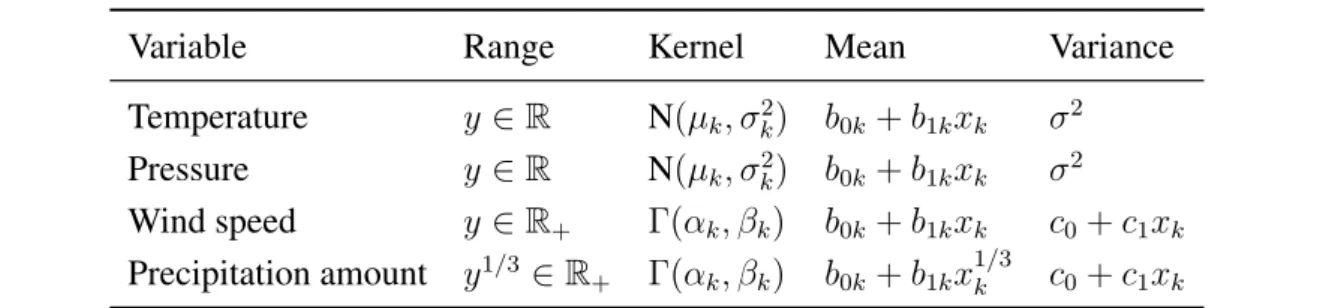
The type of distribution assumed for the kernelgkis not a feature estimated within the BMA procedure. It needs to be specified by the user and the choice depends on the weather variable of interest. Raftery et al. (2005) propose the application of BMA to surface temperature and sea level pressure. They apply Gaussian kernels in both cases. Sloughter et al. (2010) consider the postprocessing of wind speed forecasts and apply gamma kernels.
Sloughter et al. (2007) develop a BMA variant for precipitation amount, utilizing a discrete-continuous mixture distribution to account for the large number of zero observations, while precipitation observations in general are non-negative. The kernel densitygk is defined in two parts. One part models the probability of zero precipitation with a (discrete) point mass at zero, the other part describes the distribution of precipitation amount given that it is non-zero. As in the latter case the distribution can be assumed to be skewed, Sloughter et al. (2007) employ a gamma kernel. The gamma distributionΓ(α, β)is parameterized in terms of a shape parameterαand a scale parameterβ. Its mean is obtained asαβ and its variance as αβ2. Sloughter et al. (2007) found that employing the cube root of the precipitation
amount yields a more appropriate model fit than a model in terms of the original amounts. They introduce the kernels gk in the overall BMA model (2.6) for the weather quantity y describing the cube root of precipitation amount as
gk(y|xk) = P(Y = 0|xk)I{y=0}+P(Y >0|xk)hk(y|xk)I{y>0}.
In this equation, hk denotes a gamma density in terms of the cube root of precipitation amount andI{y∈A} the indicator function withI{y∈A} = 1ify ∈ Afor a desired setA and
I{y∈A} = 0fory6∈A.
The probability of zero precipitation is modeled with a logistic regression approach where the predictor variable is defined as cube root of the original forecasts
P(Y = 0|xk) = exp(a0k+a1kx 1/3 k +a2kδk) 1 + exp(a0k+a1kx 1/3 +a2kδk)
Variable Range Kernel Mean Variance Temperature y∈R N(µk, σk2) b0k+b1kxk σ2 Pressure y∈R N(µk, σk2) b0k+b1kxk σ2 Wind speed y∈R+ Γ(αk, βk) b0k+b1kxk c0+c1xk Precipitation amount y1/3 ∈ R+ Γ(αk, βk) b0k+b1kx 1/3 k c0+c1xk
Table 2.1: The ensemble BMA kernel functions for different weather variables and the associated link functions for mean value and variance
withδk = 1ifxk = 0andδk = 0otherwise. Although the BMA model of Sloughter et al. (2007) is defined for the cube root of the precipitation amount, the resulting probabilistic forecast can easily be expressed in terms of the original amounts.
Table 2.1 is taken from Möller et al. (2013), where the BMA methodology is reviewed. It gives an overview on the four most popular BMA models for the quantities temperature, pressure, wind speed, precipitation amount and their model properties. The estimation pro-cedure for the BMA models summarized in Table 2.1 are implemented in the R package
ensembleBMA(R Development Core Team, 2011; Fraley et al., 2011).
The (member specific) bias correction parameters b0k and b1k specifying the mean of the kernelgk are estimated with linear regression of the observations on the forecasts from the training data. In case of precipitation amount, the parameters for the probability of zero pre-cipitation part, a0k, a1k anda2k, are estimated by logistic regression. The weights wk, the varianceσ2, and in case of wind speed and precipitation, the variance parametersc0andc1,
are estimated by maximum likelihood from the training data. As the likelihood cannot be an-alyzed analytically, an EM-algorithm is employed by introducing the unobserved quantities
zkst = 1if ensemble memberkis the best for observation sitesat time pointtandzkst = 0 otherwise. For each(s, t)only one of the {z1st, . . . , zmst} is equal to 1, all others are zero. The estimate for σ2 obtained by the EM algorithm can then be refined so that the CRPS is minimized for the training data. For this, a numerical search over a range of values of σ2
is performed while all other parameters remain fixed. For details on how the estimation is conducted for a specific BMA model, see Raftery et al. (2005), Sloughter et al. (2007) and Sloughter et al. (2010).
Other variants of the ensemble BMA method are available that will not be discussed here, see for example the work by Roquelaure and Bergot (2008), Bao et al. (2010), and Chmielecki and Raftery (2010).
As for the EMOS model, there exists a global and a local BMA version, where on a given day either only one set of parameters is estimated over all locations or a separate set of parameters is provided for each station individually.
2.1.3
Geostatistical Output Perturbation Method (GOP)
Gel et al. (2004) introduced a quite different postprocessing approach than the others de-scribed above. Methods like EMOS and BMA are employed to perform postprocessing of an ensemble of forecasts. The forecast ensemble is available from large weather centers running the numerical models and the postprocessing is applied to improve the predictive quality of the ensemble.
In contrast to this, the Geostatistical output perturbation method (GOP) aims at producing probabilistic weather forecasts from a single numerical model, instead of postprocessing an already existing ensemble of forecasts. This method applies to whole weather fields simul-taneously rather than just to weather events at individual locations. As BMA and EMOS, GOP is designed for univariate weather quantities and fixed forecast horizons. However, in contrast to these two methods it incorporates spatial dependencies between forecast errors at different locations.
The basic idea behind GOP is to perturb output from the numerical model, instead of going down the traditional road of perturbing model inputs to obtain an ensemble. This basic idea is not necessarily including spatial correlation. As actual error fields show substantial spatial correlation, the idea of GOP is to account for this by modeling errors using a geostatistical model preserving the spatial correlation structure of the weather field. Spatially consistent ensembles of forecasts fields can easily be generated by simulating a desired number of real-izations from the resulting spatial random field model. The idea for developing this method originally came from the fact that generating a mesoscale forecast ensemble was typically not feasible for smaller weather organizations that perform mesoscale weather prediction locally without the computing resources of national weather centers.
Gel et al. (2004) consider a weather quantityY(s)at a spatial points∈R2verifying at a time
pointt, for a given forecast horizon andX(s)denotes the forecast for this quantity. The focus lies on forecasting the spatial fieldY={Y(s), s∈S}for all pointsson a large but finite set of locationsS simultaneously using the spatial field of forecastsX ={X(s), s ∈S}, while the forecast horizon and the time pointt remain fixed. The goal is to get jointly calibrated probabilistic forecasts of the whole weather field, rather than just forecasts that are calibrated
at each of the individual locations. In the GOP model of Gel et al. (2004), the finite setScan be distinct model grid points as well as observation locations.
To forecast Y(s), a finite set of variables Z(s) that are related to forecast bias might be included in the model. They can for example be functions of time (e.g. time of year or time of day) or functions of space, like latitude, longitude, altitude, land use type and others. The general form of the model for predictingY(s)proposed in Gel et al. (2004) is then given as
Y(s) = b00Z(s) + (b01Z(s))X(s) +ε(s). (2.7) Hereb0andb1are parameter vectors, whileε(s)is a Gaussian stationary space-time process
with mean zero and covariance matrixΣ. Furthermore,b00Z(s)is an additive bias-correction term andb01Z(s)a multiplicative one.
For the spatial error fieldε(s), Gel et al. (2004) assume that
1 2 Var(ε(si)−ε(sj)) = ρ 2+τ21−exp− ||si−sj|| r , (2.8)
where|| · ||is the Euclidean norm andsi 6= sj are locations in the setS. The parameterρ2 is called the nugget effect, describing the measurement error variance of the observations,
ρ2+τ2is the marginal variance ofε(s)andris a range parameter, indicating the rate at which
the spatial correlations of the errors decay. In terms of a geostatistical model, Equation (2.8) implies that the error field has an exponential variogram (Gelfand et al., 2010; Diggle and Ribeiro Jr., 2010)
γ(d) = ρ2+τ2(1−e−d/r), (2.9)
whered = ||si−sj||denotes the Euclidean distance between locationssi andsj, i 6= j, as in Equation (2.8).
Gel et al. (2004) propose a three-stage estimation method that approximates a full maximum likelihood approach to estimate the parameters in (2.7) and (2.8).
The GOP method allows for generating a spatial forecast ensemble of any desired size by simply simulating realizations from the process defined through (2.7) and (2.8). It is im-plemented in theRpackageProbForecastGOP. For the simulation, the current forecast
X(s)and the parameters estimated from past data are needed.
The original GOP method is not belonging to the class of methods with spatially varying parameters. Spatial correlations are introduced by dressing the outputs of numerical weather models with spatially correlated error fields produced by a geostatistical model, where the
parameters are estimated globally. However, the possibility to generate spatially calibrated field forecast ensembles from the output of numerical models is a useful tool.
A disadvantage of the method proposed by Gel et al. (2004) is the fact that the technique does not honor the flow-dependent information of a forecast ensemble, as it only employs a single numerical forecast for the postprocessing (e.g. a single ensemble member). BMA and EMOS on the contrary account for the information of the full ensemble. However, the basic methods are not designed to include spatial correlations between forecast errors in the model. Therefore a natural extension is to combine both types of methods. The next section presents such an extension.
2.1.4
Spatial BMA
Berrocal et al. (2007) introduced the spatial BMA technique, which combines the standard BMA and GOP approaches, thus taking advantage of the benefits of both methods. Spatial BMA resembles the original BMA technique, the predictive PDF is a weighted average of the individual forecast densities with weights reflecting the skill of the forecast members.
However, in the spatial BMA model the forecast PDFs are multivariate densities with covari-ance structures that reflect the spatial dependency of the real observations. The technique has the ability to generate statistical ensembles of whole weather fields simultaneously, of any desired size, similar to GOP. At the same time spatial BMA reduces to the original BMA at any individual location, while it reduces to the original GOP method if only an ensemble of sizem = 1is considered, that is, when a single deterministic forecast is employed.
Berrocal et al. (2007) obtain the spatial BMA forecast members by dressing the weather field forecasts of the ensemble members with simulated spatially correlated error fields, in proportions corresponding to the BMA weights of each individual member.
LetY = {Y(s), s ∈ S}denote an observational weather field for a large but finite set of locationsS and consider the m ensemble forecast fieldsX1 = {x1(s), s ∈ S}, . . . ,Xm = {xm(s), s ∈ S}. Denote byn the dimension of the finite set of locationsS. In this setting,
x1(s), . . . , xm(s), s ∈ S are the m (univariate) ensemble forecasts at location s and Y(s)
is the random variable describing the observational field at locations, with corresponding realizationys.
The predictive PDF of the fieldYis modeled as f(Y|X1, . . . ,Xm) = m X k=1 wkgk(Y|Xk). (2.10)
The parameters are the same as in the original BMA technique with the only difference being that the conditional PDFs are multivariate densities, while the densities are univariate in the original BMA technique. Similar to the univariate BMA version a multivariate normal distribution can be assumed for the kernel densities gk in case temperature or pressure is considered. The densitiesgkare centered at the bias-corrected forecast fields,b0k1+b1kXk, where1denotes the vector of ones with dimension equal to the dimension of the fieldY.
In case of kernel densities having a multivariate normal distribution, Equation (2.10) indi-cates that the predictive multivariate distribution of the weather field Y given one of them
ensemble field forecasts is multivariate normal with the following appearance:
Y|Xk ∼Nn(b0k1+b1kXk,Σ∗k), (2.11) where Σ∗k is a spatially structured covariance matrix and Nn(b0k1+ b1kXk,Σ∗k) denotes the n-variate normal distribution of its arguments. Berrocal et al. (2007) showed that the matrix Σ∗k for member k can be derived from the original BMA model variance σ2, the GOP variance parametersρ2k,τk2and the GOP covariance matrixΣkwhen applying GOP to memberk. The resulting representation of the covariance matrix is the following:
Σ∗k= σ 2 ρ2 k+τk2 Σk. (2.12) The factor αk = σ 2 ρ2
k+τk2 describes the ratio of the BMA variance to the GOP variance of
memberk for the errors. It is therefore called deflation factor for memberk. The deflation factor stems from the assumption of forecast member k being the best in the ensemble. In the original GOP approach no such assumption is necessary, as only a single forecast is considered.
For the estimation of the full set of parameters of spatial BMA it is necessary to first fit the original BMA model. Given the estimates for the BMA parameters, the GOP model is fitted for each ensemble member separately. By combining the estimates from both procedures, the full set of spatial BMA parameters is obtained.
After parameter estimation it is possible to obtain a spatial BMA ensemble of any desired size by repeatedly choosing a random numberk ∈ {1, . . . , m}and then drawing a sample from (2.11) for the chosenk. This sample is generated by dressing the bias-corrected weather
field forecastsb0k1+b1kXkwith simulations from the spatially structured conditional error fields defined through the geostatistical model. For details on this sampling procedure see Berrocal et al. (2007).
The method described in Berrocal et al. (2007) was designed for weather quantities with a multivariate normal distribution. In Berrocal et al. (2008) a similar spatial postprocessing procedure was developed for precipitation amount, where the authors adapted the univariate BMA version for precipitation amount proposed by Sloughter et al. (2007).
Recently a similar extension was developed for the basic EMOS model. The method is called spatial EMOS in analogy to spatial BMA. It combines the standard EMOS model with GOP and accounts for extending the specific EMOS variance to a spatially structured covariance matrix. For details on this method see Feldmann (2012).
2.1.5
Geostatistical Model Averaging (GMA)
Kleiber et al. (2011a) modify the global BMA method to obtain a locally adaptive technique, called Geostatistical model averaging (GMA). This method estimates biases and variances at the observation stations and interpolates them to arbitrary points on the model grid with a geostatistical model. Kleiber et al. (2011a) apply the method to temperature forecasts, where the predictive distribution can be assumed to be normal. The authors devoted further research to the GMA model and modified it for application to quantitative precipitation (Kleiber et al., 2011b).
Lets = s1, . . . , sn ∈ R3 denote a set of n training locations, x1st, . . . , xmst anm member
forecast ensemble at location s, valid at time point t, and yst the corresponding verifying observation.
Generalizing Raftery et al. (2005), the bias-correction coefficients and the variance are de-fined to vary not only by member and time point, but also by location. Therefore, GMA is an approach that uses spatially varying parameters. Concerning the bias correction parameters, Kleiber et al. (2011a) use a simplified version of the basic BMA model with only an additive bias-correction term:
yst =xkst−aks+εst, (2.13)
where aks denotes an additive bias-correction parameter for member k at site s, xkst the forecast of memberk for(s, t)andεst ∼ N(0, σs2). The error termεst is assumed to have a spatially varying variance not depending on the time indext.
The GMA predictive density is given by f(yst|x1st, . . . , xmst) = m X k=1 wkgk(yst|xkst), (2.14)
and the predictive distribution of the quantity ygiven thekth ensemble member at location
sand time pointtreads
yst|xkst ∼N(xkst−aks, cσs2), (2.15) whereσ2
s = exp(νs). The variance deflation factorcis supposed to improve the calibration of the forecast densities. Following Raftery et al. (2005), a common variance σ2
s among all members is used, andaksandσ2s are estimated from training data as
ˆ aks = 1 T T X t=1 (xkst−yst) (2.16) ˆ σs2 = 1 mT T X t=1 m X k=1 (xkst−yst−¯es)2. (2.17)
In these equations, T denotes the length of the training period ande¯s is the average of the
m×T errorsest =xkst−yst.
The empirical estimates{ˆaksi}
n
i=1 are viewed as a sample drawn from a stationary Gaussian
random field with meanµak and covariance function
Cak(si, sj) =C(ak,si, ak,sj) =ρ 2 ak+τ 2 ak exp −||si−sj|| ra1k −|h(si)−h(sj)| ra2k , (2.18)
where|| · ||is the Euclidean norm,ρ2
ak is the nugget effect describing the measurement error,
τ2
ak is a variance parameter, ra1k is the range corresponding to horizontal distance, ra2k the
range corresponding to vertical distance andh(s)is the elevation at locations.
The estimates forνs = log(σs2)areνˆs = log(ˆσ2s). In a next step the{νˆsi}
n
i=1 are viewed as
a partial realization from a stationary Gaussian random field with meanµνk and covariance matrix Cν(si, sj) = C(νsi, νsj) =ρ 2 ν +τ 2 ν exp −||si−sj|| rν1 − |h(si)−h(sj)| rν2 . (2.19)
The parameters of the random fields are estimated by maximum likelihood, using {ˆaksi}
n i=1
and{νˆsi}
n
i=1 (estimated from the training data at thenlocations) as data. Estimation has to
estimated with the EM algorithm, similar to the global BMA model. The predictive distri-bution at a locationsfor time pointtis then given by (2.14), with the estimated parameters plugged in. However, this only holds for locationss that are training sites. For other loca-tionss0there are no direct estimates ofaks0 andσ
2
s0. To obtain the predictive distribution for
ys0t at a locations0 not present in the training data, the geostatistical interpolation method
kriging (Cressie, 1993; Stein, 1999) is employed to get estimates foraks0 andνs0 at the
un-known sites0. Plugging in these estimates in (2.14) for the locations0 yields the predictive
distribution forys0t.
In contrast to GOP and spatial BMA, GMA first estimates forecast error characteristics in a spatially adaptive way at the available observation stations and then interpolates the estimates to unknown locations using kriging. With this technique, it is possible to compute forecast errors and the postprocessed predictive density at any arbitrary location, not only at the in-sample observation locations. However, the basic GMA model is not designed to in-sample ensembles of spatially correlated weather fields, as GOP or spatial BMA.
2.1.6
Ensemble Copula Coupling (ECC)
Many of the presented postprocessing methods are designed to be applied to a single weather quantity at a fixed location and for a fixed forecast horizon. They are not able to account for dependence structures between weather quantities or spatial and temporal dependencies. The ensemble forecasts on the other hand may capture many of these multivariate depen-dence structures present in the weather and climate processes, as they are solutions of the discetized differential equations describing the physics of the atmosphere. When individu-ally postprocessing the univariate margins, one may fail to retain the dependence structure present in the ensemble forecasts. This implies a need for multivariate postprocessing and research has already been conducted in this direction. Methods such as spatial BMA and spatial EMOS extend the basic BMA and EMOS methods to account for spatial structures in forecast errors and forecast variances. Other parametric models, for example to postprocess bivariate wind vectors (Schuhen et al., 2012; Pinson, 2012; Sloughter et al., 2013) account for a special case of inter-variable dependency.
The ECC approach discussed in this section is more general with respect to the type of de-pendency that is considered. It can be applied to incorporate inter-variable as well as spatial or temporal dependencies. The general formulation allows for considering all dependence structures simultaneously.
The approach was developed in Schefzik (2011) and investigated further in Schefzik et al. (2013). It utilizes the information present in the rank structure of the original raw ensemble. As the raw ensemble represents some of the true multivariate dependence structures of the atmosphere, incorporating its information in the postprocessing procedure typically leads to an improvement in predictive performance.
ECC is a multi-stage procedure resulting in a postprocessed ensemble of the same sizemas the raw ensemble. This procedure can be seen as a multivariate postprocessing method, being able to preserve dependence structures between different weather quantities as well as spatial and temporal dependence structures. This is achieved by individually postprocessing the margins of the considered multivariate forecasts and then reorder them according to the rank structure of the raw ensemble. The approach is flexible in that the postprocessing method for the margins can be chosen as desired. There is no restriction to a certain method.
Letxl1, . . . , xlm, l = 1, . . . , L, denote thel-th univariate margins of the raw ensemble. Here,
l may indicate a multi-index, l = (i, s, t), for weather quantity i = {1, . . . , I}, location
s = {1, . . . , N}and forecast horizont ={1, . . . , T}, in case of considering several
multi-variate variables simultaneously. However, ECC allows to fix one or more of these indices and consider only specific types of all possible dependencies. Then the ECC postprocessed ensemble can be generated as follows:
• Univariate postprocessing: For each margin lapply a univariate postprocessing tech-nique to the raw ensemble
xl1, . . . , xlm (2.20)
and obtain a postprocessed predictive distribution Fl. The univariate postprocessing method utilized can be selected according to the user’s needs.
• Quantization: Draw a discrete sample of sizem,
˜
xl1, . . . ,x˜lm, (2.21)
from each univariate postprocessed predictive distributionFl.
• Reordering: Determine the permutation σl of the integers{1, . . . , m}induced by the order statistics of the raw ensemble, xl(1), . . . , xl(m), for each margin l. The permu-tation is defined by σl(k) = rank(xlk) fork = 1, . . . , m. In case of ties among the ensemble members the ranks are allocated randomly. Then thel-th margin of the ECC postprocessed ensemble is given by
ˆ xl1 = ˜xl(σ l(1)), . . . ,xˆ l m= ˜x l (σl(m)). (2.22)
The discrete sample drawn in the quantization step can be generated in different ways. Schefzik et al. (2013) propose three different generation methods. The first method takes equidistant quantiles from the distributionFland is therefore called ECC-Q:
˜ xl1 =Fl−1 1 m+ 1 ,x˜l2 =Fl−1 2 m+ 1 , . . . ,x˜lm =Fl−1 m m+ 1 . (2.23)
The second method, called ECC-R, is just drawing a simple random sample
˜ xl1 =Fl−1(u1), . . . ,x˜lm =F −1 l (um), (2.24) whereu1, . . . , um iid ∼Unif[0,1].
The third method, the ECC-T, is a quantile transformation approach. It fits a parametric con-tinuous cumulative distribution functionSl to the raw ensemble margin. Then the quantiles fromFl that correspond to the percentiles of the raw ensemble values inSl are extracted, so that
˜
xl1 =Fl−1(Sl(xl1)), . . . ,x˜lm =F −1
l (Sl(xlm)). (2.25)
For details on the sampling procedures see Schefzik et al. (2013). These authors also state that the ECC-Q approach is the most favorable, due to theoretical aspects as well as due to the experiences in their case study comparing the predictive performance of the three sampling methods.
A huge advantage of the ECC approach is its low computational cost. The modeling of the multivariate dependence structure of the considered quantities can be performed by only calculating marginal ranks.
Schefzik et al. (2013) show that the ECC method can be interpreted as a nonparametric empirical copula approach. How they define an empirical copula in the context of ECC is briefly summarized below.
Let{(x1
k, . . . , xLk)|k = 1, . . . , m}denote a data set of sizem taking values inRL.
Assum-ing that there are no ties, denote by rank(xl
k) the rank of xlk within xl1, . . . , xlm. Then the corresponding empirical copulaEm is defined as
Em i1 m, . . . , iL m = 1 m m X k=1 I{rank(x1
k)≤i1,...,rank(xLk)≤iL} (2.26)
for integers0≤i1, . . . , iL ≤mand the indicator functionIAwithIA= 1on the chosen set
Let then R1, . . . , RL denote the corresponding marginal empirical cumulative distribution functions of the raw ensemble, which take values in the set Im = {0,m1, . . . ,m−m1,1}. The multivariate empirical cumulative distribution function R of the raw ensemble is defined as the mapping R : RL → Im. Then there exists a uniquely defined empirical copula
Em :ImL →Im such that
R(y1, . . . , yL) = Em(R1(y1), . . . , RL(yL)), (2.27)
for ally1, . . . , yL ∈ R. Additionally, letF˜ andFˆ denote the multivariate cumulative distri-bution functions of the quantized independently postprocessed ensemble (2.21) and the ECC postprocessed ensemble (2.22), respectively. The marginal empirical cumulative distribution functions of the quantized independently postprocessed ensemble are denoted byF˜1, . . . ,F˜L,
the corresponding copula denoted byE˜m. Then, Schefzik et al. (2013) show that
˜
F(y1, . . . , yL) = E˜m( ˜F1(y1), . . . ,F˜L(yL)) (2.28)
ˆ
F(y1, . . . , yL) = Em( ˜F1(y1), . . . ,F˜L(yL)), (2.29)
for ally1, . . . , yL ∈R. Therefore, the quantized independently postprocessed ensemble and the ECC ensemble have the same margins, while the raw ensemble and the ECC ensemble have the same copula. The relationships to empirical copulas and the corresponding theoret-ical background are investigated further in Schefzik (2013).
Chapter 3 presents some basic and fundamental facts on parametric copulas along with ex-amples of statistical approaches employing copulas. Chapters 4 and 5 introduce two different ways of combining a parametric Gaussian copula with a univariate postprocessing method.
2.2
Verification methods
This section presents methods to verify or assess the predictive quality of probabilistic fore-casts, e.g. obtained from a statistical postprocessing method.
An important aim of probabilistic forecasting was stated for example in Gneiting et al. (2003), Gneiting et al. (2005) and Gneiting et al. (2007), and picked up by many others. Gneiting et al. (2005) characterize the main issue of probabilistic forecasting as follows:
“The goal of probabilistic forecasting is to maximize the sharpness of the fore-cast PDFs subject to calibration (Gneiting et al., 2003). Calibration refers to the
statistical consistency between the forecast PDFs and the verifications and is a joint property of the predictions and the verifications.[...] Sharpness refers to the spread of the forecast PDFs and is a property of the predictions only.[...] The more concentrated the forecast PDF, the sharper the forecast, and the sharper the better, subject to calibration.”
Proper scoring rules play an important role in assessing forecasts as they address sharpness and calibration simultaneously. One example for a proper scoring rule is the CRPS men-tioned in Section 2.1.1, which will be explained in more detail here.
As this work considers univariate as well as multivariate forecasts, verification tools for both cases are introduced.
Probabilistic forecasts can take the form of a discrete distribution associated with the forecast ensemble or of a full (continuous) predictive distribution, e.g. derived from the ensemble by employing a postprocessing method. When having a full predictive (postprocessed) distri-bution, it is nonetheless possible to sample a discrete ensemble of any desired size from this distribution. Therefore verification methods designed for a forecast ensemble can indi-rectly be applied to postprocessed distributions as well, by generating an ensemble from the respective distribution.
2.2.1
Calibration
Calibration describes the consistency between the ensemble forecasts or other probabilistic forecasts and the verifying observations. It is also referred to as reliability. A simple example can explain the basic idea of reliability: If the occurrence of precipitation is predicted to have probabilitypin certain circumstances and it really occurs with a frequency of (nearly) pin these circumstances, then the forecast is said to be reliable (Candille and Talagrand, 2005; Hamill, 2001). Calibration is a joint property of the forecasts and the observations.
Univariate calibration
To assess the calibration of a univariate probability distribution, the (relative) frequencies of the Probability Integral Transform (PIT) values can be plotted in equidistant bins. This representation of the frequencies of the PIT values is called the PIT histogram. The univariate ensemble forecasts are assessed with a discrete version of the PIT histogram, the Verification
rank histogram (VRH). The VRH can be employed to assess an ensemble sampled from a full predictive distribution as well.
The basic idea of the PIT histogram is the assumption of a true (univariate) probability dis-tribution F for the weather quantity considered (Dawid, 1984; Gneiting et al., 2007). An observation ycan then be interpreted as a random sample from that true distribution. If the predicted distribution F0 is identical to the true distributionF, the predictive CDFF0 eval-uated at an observationy, p = F0(y), is a realization of a uniform distribution on [0,1]. In this case the plot obtained by computing the valuespfor all available observations and sort them into bins on the interval [0,1] produces a uniform histogram. Departures from unifor-mity can indicate that the predictive distribution is uncalibrated in some way. The number of bins on [0,1] used to obtain the PIT histogram can be chosen as desired, as long as they are equidistant.
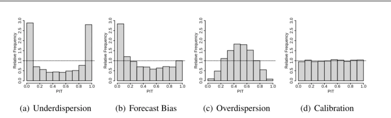
There are some rules of thumb for the interpretation of different kinds of departure from uniformity. A U-shaped histogram can be seen as indicator for a predictive distribution with too small spread compared to the spread of the observations (underdispersion), while a hump-shaped histogram indicates the opposite, a distribution with too large spread (overdis-persion). A skewed histogram indicates a biased predictive distribution.
Although the theory indicates that a well calibrated predictive distribution displays a uniform PIT histogram (or VHR histogram, see below), Hamill (2001) showed that an uncritical use of the histograms can lead to incorrect conclusions on the predictive distribution or the en-semble. Applying the principle of maximizing sharpness subject to calibration (Gneiting et al., 2007), further measures of predictive quality need to be employed to identify the pre-dictive distribution/ensemble with the best qualities. In either case it is important to interpret the PIT (and VRH) histograms with care.
To illustrate possible appearances of the histograms, Figure 2.1 shows different shapes of PIT histograms. The U-shaped histogram in panel (a) indicates underdispersion, the skewed U-shape in panel (b) often appears when the predictive distribution exhibits a strong bias, the hump-shaped histogram in panel (c) is an indicator for overdispersion, while a nearly uniform PIT histogram like the one in panel (d) indicates a well calibrated predictive distribution.
To assess the calibration of a univariate forecast ensemble x1, . . . , xm, xi ∈ R, for a real-valued univariate weather quantity, the verification rank histogram (VRH) or Talagrand di-agram (Anderson, 1996; Hamill and Colucci, 1997; Talagrand et al., 1997; Hamill, 2001; Candille and Talagrand, 2005) can be employed.