Modeling multivariate ocean data using asymmetric copulas

Title

Modeling multivariate ocean data using asymmetric copulas

Author(s)

Zhang, Yi; Kim, Chul-Woo; Beer, Michael; Dai, Huliang;

_{Soares, Carlos Guedes}

Citation

Coastal Engineering (2018), 135: 91-111

Issue Date

2018-05

URL

http://hdl.handle.net/2433/235494

Right

© 2018. This manuscript version is made available under the

CC-BY-NC-ND 4.0 license

http://creativecommons.org/licenses/by-nc-nd/4.0/; The

full-text file will be made open to the public on 01 May 2020 in

accordance with publisher's 'Terms and Conditions for

Self-Archiving'.; This is not the published version. Please cite only

the published version. この論文は出版社版でありません。

引用の際には出版社版をご確認ご利用ください。

Type

Journal Article

Textversion

author

1

Modeling multivariate ocean data using asymmetric copulas

1

2

Yi Zhanga,*, Chul-Woo Kima, Michael Beerb, Huliang Daic, Carlos Guedes Soaresd 3

a _{Department of Civil and Earth Resources Engineering, Graduate School of Engineering, Kyoto}

4

University, Japan

5

b _{Institute for Risk and Reliability, Leibniz Universität Hannover, Germany / Institute for Risk and}

6

Uncertainty, University of Liverpool, UK / Shanghai Institute of Disaster Prevention and Relief, Tongji

7

University, China

8

c _{School of Civil Engineering and Mechanics, Huazhong University of Science and Technology,}

9

China

10

d_{Centre for Marine Technology and Ocean Engineering (CENTEC), Instituto Superior Técnico,}

11

Universidade de Lisboa, Portugal

12

Abstract 13

Multivariate descriptions of ocean parameters are quite important for the design and risk assessment of

14

offshore engineering applications. A reliable and realistic statistical multivariate model is essential to

15

produce a representative estimate of the sea state for understanding the ocean conditions. Therefore, an

16

advanced modeling of ocean parameters helps towards improving ocean and coastal engineering practices.

17

In this paper, we introduce the concepts of asymmetric copulas for the modeling of multivariate ocean data.

18

In contrast to extensive previous research on the modeling of symmetric ocean data, this study is focused

19

on capturing asymmetric dependencies among the environmental parameters, which are critical for a

20

realistic description of ocean conditions. This involves particular attention to both nonlinear and

21

asymmetrically dependent variates, which are quite common for the ocean variables. Several asymmetric

22

copula functions, capable of modeling both linear and nonlinear asymmetric dependence structures, are

23

examined in detail. Information on tail dependencies and measures of asymmetric dependencies are

24

* _{Corresponding author. Tel.: +81-075-383-3421} E-mail address: [email protected]; (Y. Zhang).

Coastal Engineering 135 (2018) 91–111 https://doi.org/10.1016/j.coastaleng.2018.01.008

2

exploited. To demonstrate the advantages of asymmetric copulas, the asymmetric copula concept is

25

compared with the traditional copula approaches from the literature using actual environmental data. Each

26

of the introduced copula models is fitted to a set of ocean data collected from a buoy at the US coast. The

27

performance of these asymmetric copulas is discussed and compared based on data fitting and tail

28

dependency characterizations. The accuracy of asymmetric copulas in predicting the extreme value contours

29

is discussed.

30

Keywords: ocean engineering, joint distribution, multivariate analysis, asymmetric copula

31

32

1. Introduction 33

Offshore and coastal structures facilitate the exploitation of the vast ocean resource, which contributes

34

significantly to technological and economic development. Compared with normal structures on land,

35

offshore structures are bulky, expensive and in most cases constructed in a complex marine environment.

36

The marine environment for offshore structures can be severe, adverse, varying and uncertain. It covers a

37

broad area of climatic factors, which generally include tide, current, wind, waves, ice and other sometimes

38

devastating events such as hurricanes. When addressing different environmental risks for the offshore

39

engineering applications designers are usually required to estimate the environmental conditions at the

40

ocean site, and usually a multivariate analysis is performed (Zhang and Cheng, 2016). For example, the

41

environmental contour method developed by Winterstein et al. (1993) is popular for this purpose. As a basis

42

to produce realistic results it requires a reliable multivariate environmental model for finding the maximum

43

system response associated with a given exceedance probability. In this context the interaction among

44

various environmental influences plays an important role. In practical applications, offshore and coastal

45

structures can suffer from severe damages because of the occurrence of critical combinations of the ocean

46

environmental variables which coexist in extreme weather events such as sea storms (Zhang and Lam, 2014;

47

2015). In turn, deficiencies in modeling their joint statistics may severely overestimate the safety and

48

effectiveness of coastal and offshore structures, hence lead to unsafe design and consequently lead to

49

expensive and unexpected catastrophes (Bitner-Gregersen, 2015; Zhang et al. 2017a,b). Particularly, the

3

modeling of the joint distribution of wave height and wave period is normally a must in marine engineering

51

applications since the sea state at a specific location primarily depends on these two ocean parameters

52

simultaneously (DNV, 2014). However, the ocean climate system is an extremely complex system that

53

contains many more natural factors from both the ocean and the atmosphere. There are various sources of

54

uncertainties and potential biases that influence the ocean conditions (Zhang and Cao, 2015). Specifically,

55

the uncertainties related to the parameter dependencies are one of the most influencing factors. It was

56

recognized that the understanding of the nonlinear dependency between ocean parameters remains one of

57

the most difficult tasks, and the statistical modeling of the multivariate ocean data remains challenging due

58

to their complicated relationships (Ewans and Jonathan, 2014).

59

Lots of attempts to cope with multivariate statistical analysis can be found in the literature, involving

60

the use of a conditional distribution model (Lucas and Guedes Soares, 2015), a bivariate logistic model

61

(Morton and Bowers, 1996), a Pareto distribution model (Muraleedharan et al., 2015) and so on. Clearly,

62

the traditional conditional joint distribution model is only applicable to the multivariate problem to a certain

63

extent. If the variables contain slightly more complex relationships such as non-constant correlation between

64

pairs of random variables (e.g. the correlation coefficient value may change at extremes), the traditional

65

joint statistical model is not appropriate any more. Therefore, many more advanced techniques have been

66

employed in the multivariate analysis. Among all the developments, the application of copulas has been

67

increasingly popular in recent years. Many initial studies have illustrated that application of copula theory

68

can produce more realistic joint models for the ocean multivariate data. De Michele et al. (2007) have

69

utilized copulas to characterize sea storms in terms of significant wave height, sea storm duration, sea storm

70

inter-arrival (waiting) time, and sea storm direction. Antào and Guedes Soares (2014) have established

71

copula based bivariate models for individual wave steepness and wave height. A similar copula model for

72

description of water levels and waves are also presented by Masina et al. (2015). Montes-Iturrizaga and

73

Heredia-Zavoni (2015) have proposed a formulation for expressing the environmental contours as functions

74

of copulas and show that the dependence structure of sea state parameters can be well presented in this

75

manner. Until recently, Jane et al. (2016) have employed the copula model to predict the wave height at a

4

given location by considering the spatial dependence of the wave height at nearby locations. In contrast to

77

the traditional joint model, a copula approach has the advantage that the dependency structure between the

78

variables can be defined independently of the choice of the marginal distribution. This flexibility is highly

79

desirable in modeling the environmental parameters as the natural factors often exhibit non-obvious

80

dependencies. Moreover, it was also found that the copula model can save numerical effort when it is utilized

81

to characterize the environmental loading in the offshore structural analysis. For instance, Zhang et al. (2015)

82

have demonstrated an approach of using a copula model to characterize the sea load for the reliability

83

analysis of a real jacket structure, which reduces the numerical effort by a factor of five. A practical guideline

84

for using a copula in the design of coastal and offshore engineering applications can be found in Salvadori

85

et al. (2014). Thorough guidelines involving the use of copulas in a structural approach are given in

86

Salvadori et al. (2015). In general, from the recent advances in coastal engineering, it is now widely

87

recognized that a copula approach is very efficient and powerful to model the statistical behavior of ocean

88

dependent variables.

89

As exciting as the copula approach is, there are some obvious issues, which need to be addressed

90

for a successful application. In former studies it was criticized that most families of parametric copulas can

91

only model data having symmetric dependency (Genest and Favre, 2007). For example, the well established

92

Archimedean copula families are all symmetric. If the data dependencies exhibit asymmetric behavior, the

93

traditional copula model may no longer be adequate. Asymmetric Archimedean copulas are discussed in

94

Grimaldi and Serinaldi (2006). Unfortunately, ocean data, fall into this category; they have been found as

95

asymmetrically dependent in various previous studies. This is especially obvious for the sea state parameters,

96

which are important for in engineering design (deWaal and van Gelder, 2005). Ignoring the asymmetric

97

effects in the modeling of ocean data can be quite critical as it affects the estimates of the response statistics

98

and eventually compromises the quality of the structural reliability assessment. A reason explaining the

99

frequent (possibly unjustified) usage of symmetric (Archimedean) copulas might be that these are the ones

100

provided by the Matlab package, the one traditionally used by maritime engineers. However,, asymmetric

101

copulas can remedy this problem. Asymmetric copulas can be constructed based on the families of

5

symmetric copulas. This compounded procedure can significantly improve the fit (Jondeau, 2016). The

103

modeling of the ocean data utilizing the asymmetric copulas has received much attention recently (Vanem,

104

2016). The well known Khoudraji-Liebscher family, introduced in (Durante and Salvadori, 2010; Salvadori

105

and De Michele, 2010), gives the possibility to construct asymmetric copulas. The application of this family

106

in a maritime context has been mentioned in Salvadori et al. (2014, 2015). De Michele et al. (2013) have

107

also used it for the modeling of drought. Besides, the conditional mixture construction (Vine copulas), first

108

introduced in maritime engineering by De Michele et al. (2007), also provides the possibility to construct

109

asymmetric copulas starting from symmetric ones. However, the theoretical concepts and procedures of

110

constructing an asymmetric copula have not yet been studied in detail. Despite this, it is recognized that

111

there are many candidate asymmetric copulas in theory. These choices provide potent features and practical

112

meaning in ocean and coastal engineering applications. This potential can readily be utilized once the

113

applicability of asymmetric copulas for the modeling of ocean data has been verified and demonstrated. We

114

aim to contribute to this development with the present real case study for demonstrating and highlighting

115

the features, merits as well as limitations associated with asymmetric copulas.

116

The remainder of this paper is organized as follows. Section 2 presents a general literature review

117

of the existing techniques in modeling multivariate ocean data. Section 3 presents the fundamental

118

knowledge of copula theory and the basic dependence measure concepts. Basic concepts of asymmetry

119

measure as well as the procedures of constructing asymmetric copula models are explained in detail in

120

Section 4. Specific asymmetric copula models for ocean data are developed in Section 5 and compared

121

against traditional parametric copula models based on collected, preconditioned ocean data. To understand

122

the features of using asymmetric copulas in the ocean data modeling, a comparative study between

123

symmetric and asymmetric copula models is presented in Section 6. The concluding remarks of this paper

124

form Section 7.

125

2．Joint statistical models for ocean data 126

Among the probabilistic models available in the literature, the most commonly recommended model

127

adopted in offshore engineering design codes is the conditional joint distribution model, which is widely

6

applied to various kinds of ocean data (Burton et al. 2001; Jonathan and Ewns et al. 2011; Ernst and Seume

129

2012). The most pertinent joint distribution model that is applied in ocean engineering is for the significant

130

wave height and peak period, which characterize the spectrum of a sea state. For instance, Guedes Soares

131

et al. (1988)and Bitner-Gregersen and Haver (1989) have demonstrated the use of a joint environmental

132

model, which was constructed based on the combination of the marginal distribution of wave height and

133

conditional distribution of the wave period. Later on, Ochi (1992) introduced a bivariate log-normal

134

distribution in the modeling of the significant wave height and peak period. Generally, these conditional

135

bivariate distribution models assume significant wave height follows a Weibull distribution while wave peak

136

period follows a log-normal distribution whose model parameters are conditional on significant wave height.

137

The primary reason for using such conditional distribution model is generally that the significant wave

138

height is the most important parameter, which affects design conditions of ocean structures whereas other

139

parameters have less influence. This also agrees well with the practice design code (DNV 2010), which

140

utilizes a bivariate conditional model for the wave height and wave period. This concept of conditional

141

distribution models can also be extended to modeling other ocean parameters.

142

Beyond these fundamental developments, many of the current studies demonstrate that the joint

143

models could be further developed. Prince-Wright (1995)showed that a multivariate model using the Box

144

and Cox transformation can model the collected ocean data well, especially under the presence of

non-145

stationarities. This has been proven through a comparative study done by Bitner-Gregersen et al. (1998), in

146

which the analysis has been applied to a dataset containing both wave and wind. Repko et al. (2004)

147

developed a bivariate model of significant wave height and peak period based on a given independent value

148

of wave steepness. A comparison of several of these approaches with maximum entropy principle, including

149

clarifying the differences and performance in estimating a return value, by utilizing a specific data set can

150

also be found in (Dong et al. 2013). Ewans and Jonathan (2014) have incorporated the offshore structural

151

response properties in the multivariate sea state parameter modeling and utilized the reliability concepts to

152

derive the response based environment contours. The conditional multivariate extreme models for ocean

153

parameters considering covariate effects in directionalities are also discussed in Jones et al. (2016). An

7

overview of different methods for multivariate modeling of ocean data such as the conditional modeling

155

approach can be found from Ferreira and Guedes Soares (2002) and Jonathan et al. (2010). Although the

156

use of a conditional joint distribution model is quite convenient, its drawback is also very obvious. That is,

157

the marginal distributions and the dependence structure are both defined within one bivariate model, which

158

reduces the degree of freedom of the model. In fact, it should be noticed that conditional models are simple

159

special cases of copula models. As explained later via the Sklar’s Theorem representation (see Section 3.1

160

and Eq. (3)), the bivariate joint density fXY is simply given by

161

( )

( )

(

)

( )

( )

( , ) , XY XY X Y X Y f x y =c F x F y ⋅ f x ⋅f y , (1) 162

where cXY (.) is the copula density, FX, FY are the univariate distribution functions, and fX, fY are the univariate

163

marginal densities. In turn, the conditional density used in conditional bivariate models is a function of the

164

copula at play, i.e.

165

( )

(

( )

( )

)

( )

| ( , ) ( | ) XY , X Y XY X Y X Y f x y f x y c F x F y f x f y = = ⋅ . (2) 166

Here, the point is that, in general, it is easier to identify/construct a bivariate copula model than a conditional

167

model, especially when the sample size is scarce. In addition, changing the marginals in a copula model is

168

easy, whereas it may be awkward in a conditional model. This point has also been mentioned by many other

169

studies, which also suggested further development of the conditional bivariate models.

170

Besides the traditional joint models, some researchers have dedicated their efforts to the study of

171

establishing multivariate models using transformation approaches. Quite popular is the Nataf transformation

172

approach to construct joint probability models in offshore engineering applications (Nataf, 1962). Wist et

173

al. (2004) have applied a Nataf model to capture successive wave heights and found that they can be well

174

approximated by this joint bivariate model. A more complicated methodology has been presented by Sagrilo

175

et al. (2011) for creating a Nataf model which includes the wave, wind and water current parameters. It is

176

also applied in a structural reliability analysis where an environmental contour is estimated from the Nataf

177

model (Silva-González et al. 2013). More recently, the maximum entropy distributions, which are developed

178

based on Nataf transformation, have been utilized in the modeling of wave height and wind speed (Dong et

8

al. 2015). The features of the approximation for the distribution of the physical variables depend on whether

180

the vector of the transformed standard normal variables is close to being multi-normal. Otherwise, it is

181

criticized that certain transformation procedures might not be necessary (Huseby et al., 2013). For

182

comparison, a 4-dimensional model was easily constructed in De Michele et al. (2007) via conditional

183

mixtures of copulas (now generalized by the so-called Vine copulas).

184

Generally, under certain conditions each of the provided models has its own advantages. Quite a

185

few of these models are flexible enough to provide a realistic characterization of ocean parameter

186

dependencies under various conditions. With the aim of advancing the field of offshore reliability

187

engineering, there is a strong need for establishing a multivariate model that can handle nonlinear

188

dependencies. We found that only little attention has been devoted to the research of non-symmetric

189

multivariate models for ocean parameters. Studies in this direction with greater depth seem useful in order

190

to improve the modeling of dependencies in ocean data.

191

192

3．Copula theory and dependence measures 193

An alternative modeling approach to the multivariate ocean data is to use copulas for constructing

194

multivariate data. Copulas provide a powerful tool for modeling multivariate data, and are widely used in

195

Finance and Economics (see, e.g., Cherubini et al. 2004; McNeil et al. 2005), as well as in Hydrology and

196

Environmental Sciences. In this latter instance, as seminal references, the following ones provide a thorough

197

survey: for a theoretical introduction see Nelsen (2006); Joe (2014); Durante and Sempi (2015), for a

198

practical engineering approach see Genest and Favre (2007); Salvadori et al. (2007); Salvadori and De

199

Michele (2007).

200

3.1 Definition and basic properties

201 202

Copula is a model, which “couples” univariate marginal distributions to form a multivariate distribution. In

203

theory, a copula model is constructed by combining the marginal distributions of variables and a specific

204

dependence structure. The formal definition of a copula as a multivariate distribution with specified

205

marginal distributions is originally introduced in Sklar’s theorem (Sklar, 1959):

9

Sklar’s Theorem: Let F be an n-dimensional distribution function with marginal distributions F1, …, Fn.

207

There exists an n-dimensional copula C such that for all x∈Rn

208

(

1, , n

)

(

1

( )

1 , , n

( )

n

)

F x K x =C F x K F x (3)

209

If F1, …, Fn are all continuous, then C is unique. Conversely, if C is a copula and F1, …, Fn are distribution

210

functions, then the function defined in Eq. (3) is a multivariate distribution function with marginal

211

distributions F1, …, Fn.

212

On account of Sklar’s theorem, it is easy to see that the copula model does not need to consider the

213

characteristics of the individual random variables in the multivariate problem. This results from the

214

probability integral transform which states that the random variables Ui=Fi(Xi) are uniformly distributed on

215

[0, 1]. Note that the probability integral transform works for continuous random variables, since Fishould

216

be invertible. In other words, the copula model is a multivariate model for all the variables after their

217

transformation through the cumulative distribution function. Copula is a multivariate cumulative

218

distribution function with uniform marginals. Hence, the domain and the range values for an n-dimensional

219

copula function are

220

[ ]

[ ]

: 0,1n 0,1

C → .

221

Compared to the other joint distribution models, the copula approach has the advantage that the

222

dependency structure between the variables can be defined independently of the choice of the marginal

223

distributions. The freedom of selecting any marginal distributions for the variables in a copula makes this

224

approach quite flexible in characterizing individual variable’s behaviors. This flexibility is highly desirable

225

in the modeling of ocean parameters as the environmental factors often show non-obvious dependencies.

226

Various kinds of parametric copula families and classes can be found in the literature, see e.g. (Hutchinson

227

and Lai 1990; Nelsen 2006; Salvadori et al. 2007; Joe 2014). Each family or class of copulas can characterize

228

a certain kind of dependence in multivariate data. Most of these copulas are used for bivariate data. However,

229

they can be expanded to a multivariate model through straightforward transformations. Examples of copulas,

230

like Archimedean copulas, are presented in Appendix B.

10 232 3.2 Dependence measures 233 234 235

To highlight the significance of the copula approach in offshore engineering applications, a detailed

236

interpretation of dependence concepts is provided herein. The dependence structure is generally the most

237

important characteristic in a copula model. The most common and convenient way for measuring the data

238

dependence is using the Pearson’s correlation coefficient ρ. It is widely applied in many statistical

239

approaches because of its simplicity and ease of handling. However, the weakness of ρ is also obvious as it

240

can only represent linear dependencies. Therefore, other concepts of dependencies such as Kendall’s τk and

241

Spearman’s ρs were introduced in the literature (Joe, 2014). Compared to Pearson’s coefficients, these two

242

dependency measure concepts are much more robust. Kendall’s τk measures the possible excess of

243

concordance/discordance in the sample, while Spearman’s ρs is a measure of the “distance” (in the L1

244

integral sense) between the chosen copula and the one modeling independent variables (see Salvadori et al.

245

(2007)). Pearson coefficient requires the existence of the second order moments, and may depend on the

246

marginals, whereas Kendall and Spearman ones are nonparametric measures of association and do always

247

exist. Furthermore, the influence of unequal variances, outliers and non-linearity, which could cause

248

distortions in Pearson’s correlation coefficient, are greatly minimized in Kendall’s τk and Spearman’s ρs. In

249

other words, from engineering point of view, Kendall’s and Spearman’s dependencies are more focusing on

250

the concordance of the ranking whereas Pearson’s dependence is focusing on the value. Copula model can

251

describe various kinds of dependencies which include association concepts such as concordance, linear

252

correlation and other related measures. A copula is thus much more flexible than traditional concepts for

253

characterizing dependencies and includes these concepts. However, there are a few issues associated with

254

traditional copulas (e.g. Archimedean copulas) when they are applied to ocean data. A key drawback is that

255

some copulas are symmetric while most ocean data display non-symmetric dependencies. The reason for

256

these asymmetric dependencies can be summarized as follows:

11

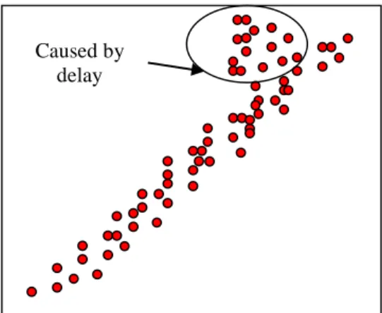
• Different ocean variables respond differently to the same environment conditions. For example, when

258

there is a hurricane, the wind speed is the most directly affected variable. A sudden increase of wind

259

speed is expected to be observed. The value of wind speed has a very quick response to the hurricane.

260

However, this effect may not be reflected in the wave height values instantaneously. There is normally

261

a delay in the observed wave height due to the change of wind speed. Such a delay causes some

262

deviations in the co-movement of wave height and wind speed time series data. Thus, a nonlinear

263

dependency is observed in the data and asymmetric dependencies evolve. This effect can be illustrated

264

by means of scatter plots as shown in Fig. 1.

265

266

Figure 1 Asymmetric dependency of ocean data caused by delay.

267 268

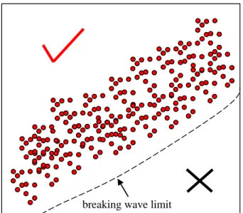
• The feasible domain of parameters restricted by the physical phenomenon is another significant reason

269

for asymmetric dependencies. For example, a large value of wave height is unlikely to be accompanied

270

by a small wave period because of the breaking wave limit. In other words, the observation of some

271

variable combinations is physically impossible. This effect is illustrated in Fig. 2. As can be seen, there

272

is no observation in the right-lower region (marked with a cross), while observations can be seen in the

273

left-upper region (marked with a tick). That is, implicit physical phenomena can limit the possibility of

274

occurrence for some data combinations. The feasible domain is therefore reduced and becomes

275 Wave height Wind speed Wave height Wind speed

Perfect linear relationship Nonlinear relationship and asymmetric dependency Caused by delay

•

•

•

• ••

•

..

•

...

.

-·

••

•

•

··'

.;. ':f •

-·

••

•

-~

..

•

.

....

-··

•••

•

•

•

••

•

-·

••

12

asymmetric.Implementing such physical feature in the copula model is not straightforward and is still

276

in its infancy stage of development.

277

278

Figure 2 Asymmetric domain of wave data caused by physical phenomenon.

279

These effects can be commonly observed in most collected ocean datasets. The ignorance of such

280

asymmetric dependencies would lead to unreliable multivariate models and associated estimates, for

281

example, of long term return values. However, the traditional copula approach is not capable of handling

282

these effects efficiently. A more advanced statistical approach is therefore required.

283

4．Asymmetric copulas 284

In general, as discussed in the above, the most commonly used copulas cannot meet the current needs for

285

modeling ocean data. An accurate modeling of the asymmetric dependencies is highly demanded. To remedy

286

this problem, we introduce several groups of asymmetric copulas as well as the basic concepts in measuring

287

the asymmetry of a copula.

288

4.1 Measure of asymmetry and tail dependency

289 290

First of all, it is necessary to introduce the basic definition of symmetry for the copula model. For a given

291

copula 𝐶𝐶(𝑢𝑢₁, … ,𝑢𝑢_𝑛𝑛), if

292

Wave height Wave period

breaking wave limit

✓

••••••

·-·

••••

···-·-=-·

....

·.--.

:.-•

· - · •• !JI

.

.

·-·

••

.

•••• • •

•••• ••

·-·

·•

-

•·-·

..

/

... ..

.

-

..

/

.

.

~·--·

.

/ ... • - · !a • • • ,,,,,,

.

..

-..

.

.

,,,,.

.

.

..

--

.

.-

. .

.

..

/ /

•• , .-...

.

.

__

·

...

-=-- •

/

,,,,,,

··--=-·--··· •...

,,,,,,

. ,~-·

·~

.-..

..

,,,,,,

/

,

__...

..

,,,.,,,.

...

.

.-.

.

, /

,,,.,

.

..

-

..

.

.

_.,,..,,. ,,,.,,,. ,,,..,,.

X

, /

13

(

1,..., i,..., j,..., n

)

( ,...,1 j,..., i,..., n)

C u u u u =C u u u u is true for any pair 𝑢𝑢_𝑖𝑖,𝑢𝑢_𝑗𝑗∈ 𝐈𝐈, 293

then ui and uj are said to be exchangeable and the copula 𝐶𝐶(𝑢𝑢₁, … ,𝑢𝑢_𝑛𝑛) is said to be symmetric (Genest and

294

Nešlehová, 2013). On the other hand, if a copula function does not satisfy the above condition, it is

295

considered to be asymmetric. Based on this idea, a measure of asymmetry in a copula was developed by

296

Klement and Mesiar (2006).

297

For instance, a natural measure of asymmetry for a 2-dimensional copula can be calculated by the

298

following equation Klement and Mesiar (2006)

299

( )

{

1 1

(

)

(

)

}

1/ 1 2 2 1 1 2 0 0 , , p p p C C u u C u u du du η =

∫ ∫

− (4) 300

where p can be set at any value that is greater than or equal to 1, 𝑝𝑝 ≥1. In other words, the measure of

301

asymmetry is represented as the distance between C and its transpose CT_{, like the norm. Moreover, it is}

302

usually more convenient to compute the value when p approaches infinity, which leads to

303

( )

( ) [ ]2

(

)

(

)

1 2 1 2 2 1 , 0,1 sup , , u u C C u u C u u η_∞ ∈ = − . (5) 304

Thus, when this measure goes up to a certain value, the copula is considered as non-exchangeable and is

305

understood to be asymmetric. In the observation of bivariate ocean data, the measure of asymmetry as

306

calculated by Eq. (5) could serve as a measure of exchangeability for the data. An extension of Eq. (4) and

307

Eq. (5) for measuring the asymmetry of two variables in high dimensional copula can also be derived as

308 following 309

( )

( , ) [ ]0,1

( )

( )

sup n C C C π π η_∞ ∈ = − u u u u , (6) 310

where u=(u1,…,un) and uπ=(uπ(1),…,uπ(n)), 𝜋𝜋 ∈ 𝑆𝑆_𝑛𝑛 is a permutation of {1,…,n}. Generally, it calculates the

311

maximal distance between a copula and a version of it where the arguments are permuted (Harder and

312

Stadtmüller, 2013).

313

Besides the measure of asymmetry, the asymmetric characteristics can also be observed from the

314

differences in the tail dependencies. According to the coefficient of tail dependence proposed by Joe (2014),

14

there are four coefficients that can be used to describe the tail dependence for bivariate data, namely, lower-316

lower, lower-upper, upper-lower, upper-upper tail dependence coefficients. For example, if an n

-317

dimensional copula 𝐶𝐶(𝑢𝑢₁, … ,𝑢𝑢_𝑛𝑛) is given, these tail coefficients can be calculated as follows:

318

( )

(

( )

( )

( )

( )

)

, 1 1 1 1 | 1 1 0 lim ,..., ,..., | l l i j i i n n j j u C P x F u x F u x F u x F u λ − − − − → + = ≤ ≤ ≤ ≤ , (7) 319

( )

(

( )

(

)

( )

( )

)

, 1 1 1 1 | 1 1 0 lim ,..., 1 ,..., | l u i j i i n n j j u C P x F u x F u x F u x F u λ − − − − → + = ≤ ≥ − ≤ ≤ , (8) 320

( )

(

( )

( )

( )

(

)

)

, 1 1 1 1 | 1 1 0 lim ,..., ,..., | 1 u l i j i i n n j j u C P x F u x F u x F u x F u λ − − − − → + = ≤ ≤ ≤ ≥ − , (9) 321

( )

(

( )

(

)

( )

(

)

)

, 1 1 1 1 | 1 1 0 lim ,..., 1 ,..., | 1 u u i j i i n n j j u C P x F u x F u x F u x F u λ − − − − → + = ≤ ≥ − ≤ ≥ − ,(10) 322

where 𝐹𝐹₁−1(. ),…,𝐹𝐹_𝑛𝑛−1(. ) are inverse marginal distribution functions for the variables x1,…,xn. Therefore,

323

these four equations provide measures of the dependence in four different tails of two variables in a

324

multivariate setting. More commonly, if a bivariate copula 𝐶𝐶(𝑢𝑢₁,𝑢𝑢₂) is analyzed, the tail dependence can

325 be derived as (Nelsen (2006)) 326

( )

(

( )

( )

)

( )

, 1 1 1|2 1 1 2 2 0 0 , lim | lim l l u u C u u C P x F u x F u u λ − − → + → + = ≤ ≤ = , (11) 327

( )

(

(

)

( )

)

(

)

, 1 1 1|2 1 1 2 2 0 0 ,1 lim 1 | 1 lim l u u u C u u C P x F u x F u u λ − − → + → + − = ≥ − ≤ = − , (12) 328

( )

(

( )

(

)

)

(

)

, 1 1 1|2 1 1 2 2 0 0 1 , lim | 1 1 lim u l u u C u u C P x F u x F u u λ − − → + → + − = ≤ ≥ − = − , (13) 329

( )

(

(

)

(

)

)

(

)

, 1 1 1|2 1 1 2 2 0 0 1 1 ,1 lim 1 | 1 2 lim u u u u C u u C P x F u x F u u λ − − → + → + − − − = ≥ − ≥ − = − . (14) 330

The value range of these four coefficients is [0, 1], i.e. 𝜆𝜆𝑙𝑙,𝑙𝑙,𝜆𝜆𝑙𝑙,𝑢𝑢,𝜆𝜆𝑢𝑢,𝑙𝑙,𝜆𝜆𝑢𝑢,𝑢𝑢∈[0,1] where a value of 0

331

indicates asymptotical independence. Equations (11) and (14) are also known as coefficients of upper and

332

lower tail dependence. For multivariate case, if the copula function is known, Eqs. (7) to (10) can be further

333 expressed as follows 334

( )

(

)

, | 0 ,..., lim l l i j u C u u C u λ → + = , (15) 335

15

( )

(

)

, | 0 ,..., lim i l u i j u C u u C u λ → + =  , (16) 336

( )

(

)

, | 0 ,..., lim j u l i j u C u u C u λ → + =  , (17) 337

( )

,

(

)

, | ₀ ,..., lim j i u u i j _u C u u C u λ → + =  , (18) 338

where 𝐶𝐶̆_𝑖𝑖(. ) and 𝐶𝐶̆_𝑗𝑗(. ) are copulas modified from the base copula 𝐶𝐶(. ) which can be shown by the following

339

relationship

340

C u_k

(

₁,...,u_n

)

=C u

(

₁,...,u_k−1,1,u_k+1,...,u_n

)

−C u

(

₁,...,u_k−1,1−u u_k, _k+1,...,u_n

)

, (19)

341

and 𝐶𝐶̆_{𝑗𝑗,𝑖𝑖}(. ) can be expressed by

342

(

)

(

)

(

)

, 1,..., 1,..., 1,1, 1,..., 1,..., 1,1 , 1,..., j i n j i i n j i i i n C u u =C u u₋ u₊ u −C u u₋ −u u₊ u . (20) 343

Tail dependencies can help to understand differences in the dependence structure for different tails.

344

This provides useful information about the properties of extreme values from the intrinsic dependencies. In

345

other words, tail dependencies provide a measure for relating one margin exceeding a certain quantile

346

threshold while the other has already exceeded that quantile threshold. When assessing the asymmetry of a

347

copula, the lower-upper and upper-lower tail coefficients can be utilized. The special case of a symmetric

348

copula is included in this model. A symmetric copula can have its variables exchanged, the copula function

349

values 𝐶𝐶(𝑢𝑢, 1− 𝑢𝑢) in Eq. (12) and 𝐶𝐶(1− 𝑢𝑢,𝑢𝑢) in Eq. (13) are identical. Further, for the symmetric case,

350

the value of the lower-upper tail coefficient equals the upper-lower tail coefficient. If these coefficients are

351

different, the copula is asymmetric. However, it should be noticed that the number of coefficients will grow

352

exponentially as the dimension increases, and the interpretation of each coefficient becomes more difficult

353

and indeterminate/vague. More detailed explanations are required when tail dependences are calculated for

354

high dimensional data.

355

4.2 Asymmetric copulas constructed by products

356 357

The construction of asymmetric copulas can be pursued in various ways. In recent years, many methods

358

have been developed in this direction (Grimaldi and Serinaldi, 2006; Mesiar and Najjari, 2014; Mazo et al.,

16

2015). These include plenty of techniques that are utilized to capture the asymmetric dependencies in the

360

multivariate data (Patton, 2006). However, not all of the asymmetric copulas can be practically applied. The

361

application of some asymmetric copulas may need extra functions to characterize the complex dependencies.

362

For instance, the well known Archimax copula, which is proposed by Capéraà et al. (2014), needs to have

363

the Pickands dependence function for its construction. The construction of Pickands dependence is quite

364

difficult and sometimes required complex statistical derivations (Pickands, 1981). Therefore, from a

365

practical point of view, the most popular and practical alternatives among these asymmetric copulas are

366

reviewed in this study. We choose to focus on the asymmetric copula families that can be easily constructed

367

from various base copulas, e.g. Archimedean copulas. Asymmetric copulas with a very complicated way of

368

construction are not explored in the present study.

369

One popular construction principle for asymmetric copulas is to formulate a product of copulas (see

370

Liebscher, (2008)). A general form to obtain an asymmetric copula is

371

(

1

)

(

1

( )

1

( )

)

1 ,..., ,..., k product n i i in n i C u u C f u f u = =

∏

, (21) 372

where 𝐶𝐶₁, … ,𝐶𝐶_𝑘𝑘: [0,1]𝑑𝑑 →[0,1] are all n-dimensional copulas, 𝑓𝑓_{𝑖𝑖𝑗𝑗}: [0,1]→[0,1] for i=1,…,k, j=1,…,n are

373

functions that are strictly increasing or identically equal to 1. To ensure this product of copulas is also a

374

copula, the functions 𝑓𝑓_{𝑖𝑖𝑗𝑗} have to satisfy the following additional properties:

375

1. 𝑓𝑓_{𝑖𝑖𝑗𝑗}(1) = 1 and 𝑓𝑓_{𝑖𝑖𝑗𝑗}(0) = 0,

376

2. 𝑓𝑓_{𝑖𝑖𝑗𝑗} is continuous on (0,1],

377

3. If there are at least two functions 𝑓𝑓_{𝑖𝑖1𝑗𝑗},𝑓𝑓_{𝑖𝑖2𝑗𝑗} with 1≤ 𝑖𝑖₁,𝑖𝑖₂≤ 𝑘𝑘 which are not identically equal to 1, then

378

𝑓𝑓𝑖𝑖𝑗𝑗(𝑥𝑥) >𝑥𝑥 holds for 𝑥𝑥 ∈(0,1), i=1,…,k.

379

From the above it is easy to see that the constructed copula is generally an asymmetric copula. The

380

properties of these asymmetric copulas are derived from the fundamental properties of copula model. All

381

the functions 𝑓𝑓_{𝑖𝑖𝑗𝑗} play a role in the asymmetric dependence modeling. This technique is also known as an

17

extension of Khoudraji’s device (1995). For example, by utilizing type I individual function (see Table 1)

383

and set k, n=2, Eq. (21) becomes exactly the Khoudraji copula. The n-dimensional copulas 𝐶𝐶₁, … ,𝐶𝐶_𝑘𝑘 can be

384

selected from various groups of parametric copulas, e.g. the Gumbel, the Clayton, the Frank, the Gaussian and 385

etc. It is also possible to use independent or Fréchet-Hoeffding bounds for the individual copulas. As for the 386

individual functions 𝑓𝑓_{𝑖𝑖𝑗𝑗}, Liebscher (2008) has provided a list of candidate functions which are suitable for the 387

application. The most applicable individual functions are presented in Table 1. This flexibility can allow this 388

asymmetric copula to be extended to much more complex multivariate models. However, even with these 389

individual functions provided, the number and type of individual copulas are still unknown and need to be decided. 390

Moreover, more advanced numerical methods are required for the simulation and use of this type of copula. 391

Fortunately, certain simulation techniques have already been developed and utilized in the statistical analysis 392

software. For example, the simulation of Khoudraji copula can be easily done by using a package named “copula” 393

in R(Hofert et al., 2016). The use of Khoudraji-Liebscher copulas has already been very popular in the

394

hydrology community, for example, both in terrestrial hydrology (e.g., Durante and Salvadori (2010); De

395

Michele et al. (2013)) and in maritime hydrology (e.g., Salvadori et al. (2013, 2014, 2015)).

396

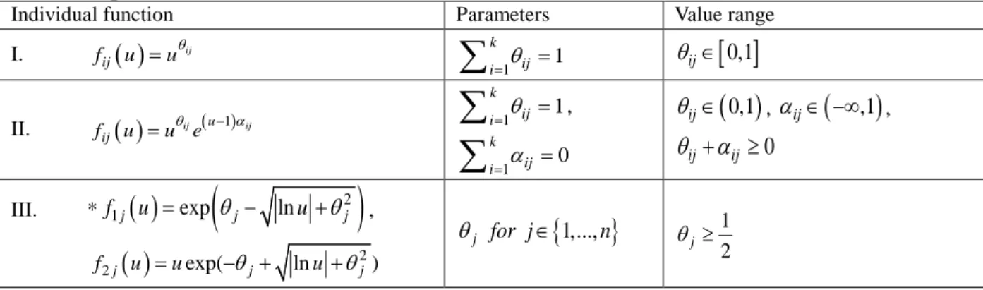
Table 1 Examples of individual functions 397

Individual function Parameters Value range

I.

( )

ij ij f u =uθ 1 1 k ij i=θ =

∑

θ_ij∈

[ ]

0,1 II.

( )

ij (u 1) ij ij f u =u eθ − α 1 1 k ij i=θ =

∑

, 1 0 k ij i=α =

∑

( )

0,1 ij θ ∈ , αij∈ −∞

(

,1

)

, 0 ij ij θ α+ ≥ III. * f1j

( )

u =exp

(

θj− lnu +θj2

)

,

( )

2 2j exp( j ln j) f u =u − +θ u +θ

{

1,...,

}

j for j n θ ∈ 1 2 j θ ≥

*Note: type III individual functions can only be used for the asymmetric copula having two individual copulas 398

(e.g. k=2). 399

400

4.3 Asymmetric copulas constructed by linear convex combinations 401

402

Another way of an algebraic construction of an asymmetric copula is by linear convex combinations of

403

copulas. However, the direct linear convex combination of copulas is not suitable to create asymmetric

404

copulas. Since most fundamental copulas are symmetric, the linear convex combination of these copulas

405

✓I

I

-✓I

I

18

would also only produce symmetric copulas. Wu (2014) has proposed a way to modify the fundamental

406

copulas in order to account for asymmetric properties. In his theorem, a new kind of copula is proposed as

407

(

1,...,

)

(

1,..., 1,1, 1,...,

)

(

1,..., 1,1 , 1,...,

)

h n h h n h h h n

C u u =C u u ₋ u ₊ u −C u u ₋ −u u ₊ u (22)

408

where C(.) is the original n-dimensional base copula. It can be seen that the variable uh is not exchangeable

409

with other variables in the developed copula. This type of copula is also known as flipped copula as specified

410

by Salvadori et al. (2007). Such copulas which have flipped dependence structures are already available in

411

the R package “copula” (e.g. rotCopula()).

412

Therefore, with such amendment, 𝐶𝐶̆_ℎ(. ) can be used to fit data exhibiting unequal tail dependencies

413

along the hth variable. Furthermore, in order to model asymmetric properties in multiple variables, one may

414

use the following equation to construct the copulas:

415

(

₁

)

(

₁

)

0 ,..., n ,..., addition n _h h h n C u u =

∑

₌ p C u u (23) 416

where 𝑝𝑝_ℎ is a weighting factor satisfying the conditions 0≤ 𝑝𝑝_ℎ≤1 and ∑𝑛𝑛_ℎ=0𝑝𝑝_ℎ= 1 . When h=0,

417

𝐶𝐶̆0(𝑢𝑢1, … ,𝑢𝑢𝑛𝑛) =𝐶𝐶(𝑢𝑢1, … ,𝑢𝑢𝑛𝑛). That is, an asymmetric copula is obtained by linear convex combinations of

418

copulas. The compound copula is now a combination of various base copulas with different individual tail

419

dependencies. As in the approach in Section 4.2, a large group of copula families can be selected for the

420

base copula 𝐶𝐶(𝑢𝑢₁, … ,𝑢𝑢_𝑛𝑛). For the case of a bivariate copula 𝐶𝐶(𝑢𝑢₁,𝑢𝑢₂), Eq. (22) can be further expressed as

421

(

)

(

)

1 1, 2 2 1 1, 2 C u u =u −C −u u , (24) 422

(

)

(

)

2 1, 2 1 1,1 2 C u u = −u C u −u , (25) 423

which can also be called the horizontal- and vertical-flipped copulas (Salvadori et al. 2007). Therefore, the

424

constructed asymmetric copula can be generally written as

425

(

1, 2

)

0

(

1, 2

)

1 1

(

1, 2

)

2 2

(

1, 2

)

addition

C u u = p C u u + p C u u + p C u u (26)

426

where 𝑝𝑝₀,𝑝𝑝₁,𝑝𝑝₂≥0 and 𝑝𝑝₀+𝑝𝑝₁+𝑝𝑝₂= 1. Using this formula, we can easily adjust the values of weight

427

factors assigned to each base copula in order to characterize the asymmetry properties of bivariate data along

428

different variables. In other words, the individual copula 𝐶𝐶̆₁(𝑢𝑢₁,𝑢𝑢₂) or 𝐶𝐶̆₂(𝑢𝑢₁,𝑢𝑢₂) can only capture the

19

asymmetry in one variable. As such, we can also point out the differences between the current construction

430

method and Liebscher’s method. That is, the current method constructs asymmetric copulas that present the

431

asymmetric property in one variable each at a time, whereas Liebscher’s method constructs the copulas for

432

variables having asymmetric properties all at a time.

433

4.4 Skewed copula

434 435

Besides the algebraic construction methods, another way of modeling asymmetrically dependent data is

436

utilizing skewed copulas. This approach originated from skewed multivariate distributions and generalizes

437

the original distribution to allow non-zero skewness. The idea is to transform a multivariate distribution to

438

an asymmetric one by introducing a parameter, which can regulate the skewness (Koll et al., 2013). However,

439

there are only few skewed copulas available in the literature. The most popular one is the skew Gaussian 440

copula.

441

Before introducing the skew Gaussian copula, we recall some basics about the Gaussian copula. An

442

n-dimensional Gaussian copula is defined by

443

(

)

(

1

( )

1

( )

)

1,..., 1 ,..., ; Gaussian n n n C u u = Φ Φ− u Φ− u Σ (27) 444

where Φ-1_{(.) denotes the inverse of the standard normal distribution function,} Φ

n(.) represents the n

-445

dimensional normal distribution function, and ∑ stands for the covariance matrix. The Gaussian copula is a

446

member of the elliptical copula family. The function is very like a multivariate normal distribution function

447

and therefore can only be used to model variables having symmetric dependencies. To overcome this

448

limitation, the basic formula is modified to account for asymmetries based on skew Gaussian distribution

449

functions. A general n-dimensional skew Gaussian copula is given by

450

(

)

(

1,

(

)

1,

(

)

)

1 1

1,..., ; , , , skew 1; 1,1, 1 ,..., skew ; ,1, ; , ,

skew Gaussian n n skew n n n

C ₋ u u µ Σ β =F F− u µ β F− u µ β µ Σ β (28)

451

where 𝐹𝐹₁−1_{,𝑠𝑠𝑘𝑘𝑠𝑠𝑠𝑠}(. ) is the inverse of the univariare skew normal distribution SN(μi, 1, βi), 𝐹𝐹_{𝑛𝑛,𝑠𝑠𝑘𝑘𝑠𝑠𝑠𝑠}(. ) is the n

-452

dimensional skew normal distribution with mean parameter μ, shape parameters β and covariance matrix ∑.

453

The density function of a multivariate skew normal distribution for n-dimensional random variables

20 X(x1,…,xn) is given by 455

(

; ,

)

2

(

; ,

)

(

T ; ,

)

n n n f X µ Σ,β = φ X µ Σ Φ β X µ Σ (29) 456

where 𝜙𝜙_𝑛𝑛(∙;𝜇𝜇,∑) and 𝛷𝛷_𝑛𝑛(∙;𝜇𝜇,∑) represent the probability density function and cumulative distribution

457

function of n-dimensional normal distribution with mean μ and covariance ∑ (Azzalini and Dalla Valle,

458

1996). Usually, for the ease of modeling, the mean values are all set at zero. The asymmetric property thus

459

only results from the shape parameters. When β=0, the copula becomes the standard Gaussian copula with

460

no skewness. If β increases, the skewness of the distribution increases. Once β changes its sign, the skewness

461

is reflected in the opposite side of the axis. The asymmetric properties can be characterized by the shape

462

parameters either for the marginals or for the multivariate distribution.

463

From the comparison between Eq. (28) and Eq. (21), it can be seen that the skew copula is in fact a

464

special case of the constructed copulas as given in Section 4.2. Compared to the general form, the skew

465

copula has only one individual copula (k=1) and this individual copula (Ci) and the individual function (fij)

466

are coming from the same family (skew Gaussian distribution). However, it is still interesting to discuss the

467

use of skew copulas since no previous work has been done on its application in the modeling of ocean data.

468

5．Data analysis 469

To demonstrate the advantages of asymmetric copulas over the other models in a real case application, a

470

comparative study is performed based on ocean data from the National Data Buoy Center, US (NDBC,

471

2016). The data were collected at a site in the Aleutian Trench, off the south coast of Alaska (52.785˚N

472

155.047˚W Buoy No. 46066) which has a water depth of 4545 m. The hourly recorded ocean data from the

473

years 2014 and 2015 are extracted for the investigation (2014/1/1 01:00-2015/12/31 23:00). We choose to

474

study three ocean parameters: significant wave height (Hw), average wave period (Ta) and wind speed (Vw).

475

The unit of the measured wave height is in meters, while the units of wave periods and wind speed are

476

second and meter per second, respectively. Here, only non-braked waves are recorded. The record of the

477

ocean data shows a clear seasonal variation as depicted in Fig. 3. The data indicate more severe conditions

478

in winter compared to summer.

21

As the time varying feature of the data record is very obvious, it is not reasonable to consider a

480

simple statistical analysis to all the multivariate data at one time. A data partitioning is necessary to separate

481

different groups of data for the analysis. To simplify the problem, we analyze a specific period of data which

482

are critical and short. On this basis we can assume that all ocean data are quasi stationary for the statistical

483

analysis. In this study, the ocean data covering the most severe period from November to February are

484

chosen for the investigation. Figure 3 shows the variations of the mean and standard deviation of Hw, Ta and

485

Vw over this period. However, the statistical testes are required to check whether the data are significantly

486

different from each other in different months. Here, t-tests are applied to test whether the data of Hw, Ta and

487

Vw are significantly different in different months. The highest p-values for Hw, Ta and Vw are 0.324, 0.187

488

and 0.443 which imply that the hypothesis of data from different months show statistically different means

489

is rejected. Therefore, it is believed that the data within the period from November to February may

490

approximately be represented by the same statistical model. Although the data within this period might not

491

be perfectly homogeneous, the time varying effects associated with Hw, Vw and Ta can be neglected.

492

Therefore, the data set (Hw, Vw, Ta) from the four months winter season in 2014 and 2015 are used for the

493

subsequent statistical analysis. However, it should be pointed out the ocean data at this ocean site for the

494

whole period is not completely collected. It has an amount of missing data in the hourly record. Only 3910

495

out of 5952 observations are collected. The detailed information and a general statistical summary of Hw,

496

Vw and Ta is provided in Table 2. The differences in statistical properties between different ocean data are

497

large. Individual characteristics of the ocean parameters Hw, Vw and Ta have to be investigated separately.

498

499 Jan Feb Mar Apr May Jun Jul Aug Sep Oct Nov Dec

8 7 6 5 4 3 2 1 0 H w ( m ) Dec Nov Oct Sep Aug Jul Jun May Apr Mar Feb Jan 20 15 10 5 0 V w ( m /s )

22 500

501

Figure 3 Monthly box plot of Hw, Vw and Ta over one year

502 503

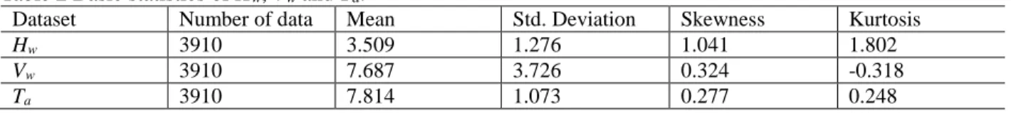
Table 2 Basic statistics of Hw, Vw and Ta.

504

Dataset Number of data Mean Std. Deviation Skewness Kurtosis

Hw 3910 3.509 1.276 1.041 1.802

Vw 3910 7.687 3.726 0.324 -0.318

Ta 3910 7.814 1.073 0.277 0.248

505

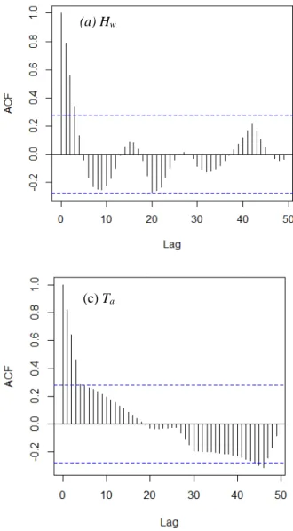
Another issue that needs to be considered before the statistical modeling is the serial correlation. To

506

observe the serial dependence, the autocorrelation functions for Hw, Vw and Ta are plotted in Fig. 4. The

507

figure shows the autocorrelation function values of the time series are not very strong when time lag is about

508

3 hours. In fact, the dependence between the observation and the one 3 hours later can be negligible (e.g.

509

autocorrelation function value is within the rejection region for test of individual autocorrelations, see Fig.

510

4). Therefore, in this study, we generally assume the serial dependence is weak and the collected data can

511

be directly used for statistical analysis. However, it should be realized the time series data need to be

pre-512

processed when serial correlation is very strong. The current analysis only adopts a relaxed assumption in

513

this data pre-processing. Typical steps about how to remove the serial correlations contained in time series

514

data can be found in Vanem (2016).

515 Dec Nov Oct Sep Aug Jul Jun May Apr Mar Feb Jan 11 10 9 8 7 6 5 4 T a ( s )

23 516

517

Figure 4 Autocorrelation function of Hw, Vw and Ta for the selected period

518

As a first step, like in all the copula approaches, marginal distributions are determined for the

519

variables to put up an asymmetric copula. In order to make a fair judgment, a group of distributions are

520

utilized to fit the individual ocean data. These include Weibull, Normal, Lognormal, Rayleigh, Extreme

521

value, Exponential and Gamma distributions. Maximum likelihood method is used to estimate the model

522

parameters for each variable. The Akaike Information Criterion (AIC) is used to select the best models.

523

Table 3 summarizes the calculated statistics for each model. It indicates the best models are Lognormal

524

distribution for Hw, Weibull distribution for Vw and Gamma distribution for Ta. The goodness of fitting of

525

these models to the variables can be seen from Fig. 5. The 95% bounds of the empirical cumulative

526 (a) Hw (b) Vw (c) Ta 0 0 co 0 (D 0 <D (() 0 0 '<I: LL '<I: (_) 0 <( N LL 0 0 <( N ci 0 ₀ 0 0 0 N c:;> 0 10 20 30 40 50 0 10 20 30 40 50 Lag Lag q ID 0 (() 0 LL ~ 0 0 <( N 0 q 0 N ci _I 0 10 20 30 40 50 Lag

24

distribution function are also included. The p-value in the Kolmogorov-Smirnov test shows that the fitted

527

model is a valid option at a significant level of 1% for each of the ocean variables.

528

529

530 531

Figure 5 Distribution fitting to the collected ocean data 532

533

Table 3 Calculated AIC statistics for the marginal distribution model fitting 534

Weibull Normal Lognormal Rayleigh Extreme

value

Exponential Gamma

Hw 125814 128922 119792* 127976 149104 156506 121004

Vw 139494* 151950 151300 187970 162430 228980 151000

Ta 186032 187578 188190 189672 198086 218644 186006*

*The lowest AIC value indicates the best model. 535

536

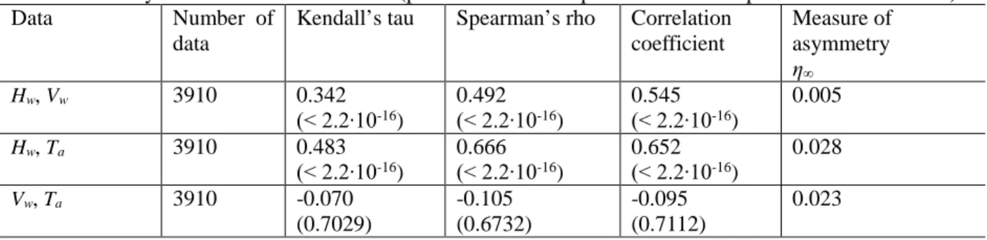
Despite the differences in the individual characteristics, the multivariate statistical properties in

537

between the ocean variables are studied. The dependence measure concepts including Kendall’s tau,

538

Spearman’s rho and correlation coefficient are calculated for each pair of the dataset as summarized in Table

539 p-value=0.0336 p-value=0.0174 p-value=0.0238 0.9 0.8

£0

_7

E 1 o.6 0 5. ., 0.5 .::: .'@ 0.4 E 8 0.3 0.2 0.1 0.9 0.8 £0.1 E " 0.6 -" 2 c.. ., 0.5 -E " 0.4 ,; E 8 0.3 0.2 0.1 0 2 3 4 5 6 7 - -Empirical CDF

··· confidence bounds (95%)

- -Lognonnal 5 6 7 H w 8 9 10 - -Empirical CDF

"""""Confidence bounds (95%)

- -Gamma 8 9 10 II 12 T a 0.9 0.8

£0_

7

E 1 o.6 2 ;o.s .::: ] 0 4 _::, . E 8 0.3 0.2 0.1 - -Empirical CDF

... confidence bounds (95%)

- -Weibull 0"""'~- - - ~ - - - - ~ - - - ~ - - - - ~ 0 5

I

I

10 V w 15 20

25

4. Furthermore, the measure of the asymmetry is computed for the paired data and presented in the table.

540

Here, the calculation of the measure of asymmetry adopts an infinity value for p as following Eq. (5). As

541

can be seen from this table, the dependence measure concepts show similar values. The dependence in (Hw,

542

Vw) and (Hw, Ta) is relatively stronger than that in (Vw, Ta) (as indicated by the value and independence tests).

543

On the other hand, the results of asymmetric measures for (Hw, Ta) and (Vw, Ta) are slightly higher than (Hw,

544

Vw). A test of exchangeability is also conducted for the bivariate data based on pseudo observations. The

545

calculated p-values for (Hw, Ta), (Vw, Ta) and (Hw, Vw) are 0.001, 0.003 and 0.008 according to the method

546

given by Genest et al. (2012). This indicates all the bivariate data show obvious asymmetric dependency. A

547

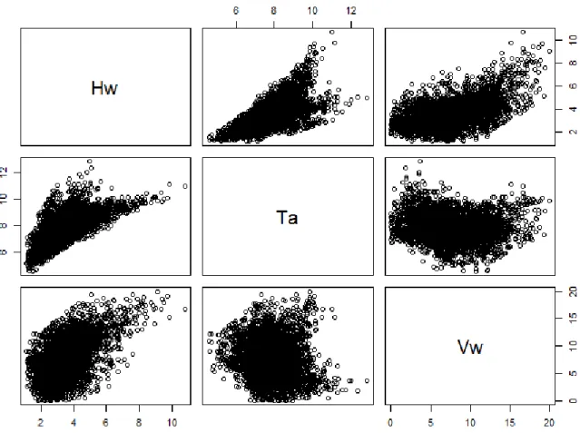
general feeling of these complicated dependencies can be developed using the scatter plot in Fig. 6. It can

548

be seen that all the dependencies between the ocean variables are not perfectly linear. For example, (Hw, Ta)

549

data points are only available in the left upper domain in the scatter plot. Moreover, it should be noticed that

550

the tail dependency of these bivariate data is quite different. (Hw, Ta) data has a very strong tail dependency

551

in the maxima extremes whereas (Hw, Vw) data has a weak tail dependency in the maxima extremes (can be

552

seen as the linearity). The characteristics of tail dependency must also be accounted for in the multivariate

553

data modeling.

554

555

Table 4 Summary of the ocean bivariate data (p-values of the independence tests are provided in the bracket) 556

Data Number of data

Kendall’s tau Spearman’s rho Correlation coefficient Measure of asymmetry η∞ Hw, Vw 3910 0.342 (< 2.2∙10-16₎ 0.492 (< 2.2∙10-16₎ 0.545 (< 2.2∙10-16₎ 0.005 Hw, Ta 3910 0.483 (< 2.2∙10-16₎ 0.666 (< 2.2∙10-16₎ 0.652 (< 2.2∙10-16₎ 0.028 Vw, Ta 3910 -0.070 (0.7029) -0.105 (0.6732) -0.095 (0.7112) 0.023