doi:10.1093/biostatistics/kxy060
Advance Access publication on October 30, 2018
Sparse relative risk regression models
ERNST C. WIT∗Institute of Computational Science, USI, Via Buffi 13, 6900 Lugano, Switzerland
[email protected] LUIGI AUGUGLIARO
Department of Economics, Business and Statistics, University of Palermo, Building 13, Viale delle Scienze, 90128 Palermo, Italy
HASSAN PAZIRA
Bernoulli Institute, University of Groningen, Nijenborg 9, 9747 AG Groningen, The Netherlands
JAVIER GONZÁLEZ†
Amazon Research Cambridge, Poseidon House, Castle Park, Cambridge, UK
FENTAW ABEGAZ
Bernoulli Institute, University of Groningen, Nijenborg 9, 9747 AG Groningen, The Netherlands and Department of Pediatrics and Systems Biology Centre for Energy Metabolism and Ageing, University of
Groningen, University Medical Center Groningen, 9700 AD Groningen, The Netherlands
SUMMARY
Clinical studies where patients are routinely screened for many genomic features are becoming more routine. In principle, this holds the promise of being able to find genomic signatures for a particular disease. In particular, cancer survival is thought to be closely linked to the genomic constitution of the tumor. Discovering such signatures will be useful in the diagnosis of the patient, may be used for treatment decisions and, perhaps, even the development of new treatments. However, genomic data are typically noisy and high-dimensional, not rarely outstripping the number of patients included in the study. Regularized survival models have been proposed to deal with such scenarios. These methods typically induce sparsity by means of a coincidental match of the geometry of the convex likelihood and a (near) non-convex regularizer. The disadvantages of such methods are that they are typically non-invariant to scale changes of the covariates, they struggle with highly correlated covariates, and they have a practical problem of determining the amount of regularization. In this article, we propose an extension of the differential geometric least angle regression method for sparse inference in relative risk regression models. A software implementation of our method is available on github (https://github.com/LuigiAugugliaro/dgcox).
Keywords: dgLARS; Gene expression data; High-dimensional data; Relative risk regression models; Sparsity; Survival analysis.
∗To whom correspondence should be addressed. †The work in this paper was done before joining Amazon.
© The Author 2018. Published by Oxford University Press. All rights reserved. For permissions, please e-mail: [email protected].
1. INTRODUCTION
Advances in genomic technologies have meant that many new clinical studies in cancer survival include a variety of genomic measurements, ranging from gene expression to SNP data. Studying the relationship between survival and genomic markers can be useful for a variety of reasons. If a genomic signature can be found, then patients can be given more accurate survival information. Furthermore, treatment and care may be adjusted to the prospects of an individual patient. Eventually, the genomic signature combined with information from other studies may be used to identify drug targets. We will focus on four recent studies of cancer survival for four different tumors. Our aim is to find a reproducible sparse predictor for cancer survival.
Sparse inference in the past two decades has been dominated by methods that penalize typically convex likelihoods by functions of the parameters that happen to induce solutions with many zeros. The Lasso (Tibshirani,1996), elastic net (Zou and Hastie,2005),l0 (Rippeand others,2012), and the SCAD (Fan and Li, 2001) penalties are examples of such penalties that, depending on some tuning parameter, conveniently shrink estimates to exact zeros. Also in survival analysis, these methods have been introduced.Tibshirani(1997) applied the Lasso penalty to the Cox proportional hazards model.Gui and Li (2005),Sohnand others(2009), andGoeman(2010) suggested important computational improvements to make the calculation of the Lasso estimator in the Cox proportional hazards model more efficient. Although the Lasso penalty induces sparsity, it is well known to suffer from possible inconsistent selection of variables.
Whereas penalized inference is convenient, justification of the penalty is somewhat problematic. Interpreting the solution as a Bayesian MAP estimator with a particular prior on the parameters seems to merely reformulate the problem, rather than solving it. Furthermore, the methods suffer from being not invariant under scale transformations of the explanatory variables. This means that measuring, e.g., height in centimeters or inches can and probably will result in dramatically different answers. Therefore, most penalized regression methods start their exposition by assuming that the variables are appropriately renormalized. This is clearly a merely algorithmic device and simply begs the question of invariance. Clearly the strongest argument in favor of some of these methods are their asymptotic properties. Nevertheless, what this means in the small sample settings encountered in practice is also problematic.
In this article, we will approach sparsity directly from a likelihood point of view. The angle between the covariates and the tangent residual vector within the likelihood manifold provides a direct and scale-invariant way to assess the importance of the individual covariates. The idea is similar to the least angle regression approach proposed byEfronand others(2004). However, rather than using it as a computational device for obtaining Lasso solutions, we view the method in its own right as inAugugliaroand others
(2013). Moreover, the method extends directly beyond the Cox proportional hazard model. In fact, we will focus on general relative risk survival models.
The remaining part of this article is structured as follows. In Section 2, we introduce the relative risk regression model and in Section3, first we derive the differential geometric structure of a relative regression model and then we use it to extend the differential geometric least angle regression (dgLARS) method (Augugliaroand others,2013). In this section, by appealing to the theory of Z-estimation, we derive a robust way of selecting a unique point of the path of solutions defined by dgLARS. In Section4, by simulation studies, we compare the performance of the proposed method to other sparse survival regression approaches, especially in the presence of correlated predictors. In Section5, we return to the motivating cancer survival studies and employ differential geometric Cox proportional hazards modelling to find a genetic signature for cancer survival in skin, colon, prostate, and ovarian cancer. Finally, in Section6we draw some conclusions.
2. RELATIVE RISK REGRESSION MODELS
In analyzing survival data, one of the most important tools is the hazard function, which is used to express the risk or hazard of failure at some timet. Formally, letT be the (absolutely) continuous random variable associated with the survival time and letf(t)be the corresponding probability density function, the hazard function is defined asλ(t)=f(t)/{1−0tf(s)ds}and specifies the instantaneous rate at which failures occur for subjects that are surviving at timet. Suppose that the hazard function can depend on ap-dimensional, possibly time-dependent, vector of covariates, denoted byx(t) = (x1(t),. . .,xp(t)). Relative risk regression models are based on the assumption thatx(t)influences the hazard function through the following relation
λ(t;x)=λ0(t)ψ{x(t);β}, (2.1)
whereβ ∈ B ⊆Rpis ap-dimensional vector of unknown fixed parameters andλ
0(t)is the base line hazard function at timet, which is left unspecified. Finally,ψ:Rp×Rp→Ris a differentiable function, called therelative risk function, and the parameter spaceBis such thatψ{x(t);β}>0 for eachβ ∈B. We also assume that the relative risk function is normalized, i.e.,ψ(0;β) =1. Model (2.1), originally proposed inThomas(1981), clearly extends the usual Cox regression model (Cox,1972) which is obtained whenψ{x(t);β} =exp{βx(t)}, and allows us to work with applications in which the exponential form of the relative risk function is not the best choice. This issue was observed inOakes(1981) and further underlined inCox(1981). As a motivating example for the generalization (2.1), several authors have noted that the linear relative risk functionψ{x(t);β} =1+βx(t)provides a natural framework within which to assess departures from an additive relative risk model when two or more risk factors are studied in relation to the incidence of a disease (see e.g.,Thomas 1981;Prentice and others1983;Prentice and Mason 1996, among the other). Other possible choices for the relative risk functions are the logit relative risk functionψ{x(t);β} = log[1+exp{βx(t)}], proposed byEfron(1977), or the the excess relative risk modelψ{x(t);β} =m=1p {1+xm(t)βm}.
Suppose thatnobservations are available and lettibe theith observed failure time. Assume that we havekuncensored and untied failure times and letDbe the set of indices for which the corresponding failure time is observed; the remaining failure times are right censored. As explained inCox and Oakes (1984), if we denote byR(t)the risk set, i.e., the set of indices corresponding to the subjects who have not failed and are still under observation just prior to timet, under the assumption of independent censoring, inference about theβcan be carried out by the partial likelihood function
Lp(β)= i∈D ψ{xi(ti);β} j∈R(ti)ψ{xj(ti);β} . (2.2)
When the exponential relative risk function is used in model (2.1) and we work with fixed covariates, (2.2) is clearly equal to the original partial likelihood introduced inCox(1972) and discussed in great detail in Cox(1975).
3. SPARSE RELATIVE RISK REGRESSION
In this section, we extend the dgLARS method (Augugliaroand others,2013) to the relative risk regression models. The basic idea underlying the dgLARS method is to use the differential geometrical structure of a Generalized Linear Model (GLM) (McCullagh and Nelder,1989) to generalize the LARS method (Efron
and others,2004). This means that, our first step is relate the partial likelihood (2.2) with the likelihood function of a specific GLM. As originally observed inThomas(1977), and studied in greater detail in
Prentice and Breslow(1978), to solve this problem we shall use the identity existing between the partial likelihood and the likelihood function of a logistic regression model for matched case–control studies. The idea to use this identity to study the differential geometrical structure of a relative risk regression model is not new and was originally used inMoolgavkar and Venzon(1987) to construct approximated confidence regions for the proportional hazards model.
3.1. Differential geometrical structure of the relative risk regression model
The partial likelihood (2.2) can be seen as arising from a multinomial sample scheme. Consider an index i ∈ D and let Yi = (Yih)h∈R(ti) be a multinomial random variable with sample size equal to 1 and cell probabilities πi = (πih)h∈R(ti) ∈ i, i.e., p(y;πi) =
h∈R(ti)π yih
ih . Assuming that the random vectors Yi are independent, the joint probability density function is an element of the set S = i∈D h∈R(ti)π yih ih :(πi)i∈D∈i∈Di
, called the ambient space. We would like to underline that our differential geometric constructions are invariant to the chosen parameterization, which means thatScan be equivalently defined by the canonical parameter vector and this will not change the results. In this article, we prefer to use the mean value parameter vector to specify our differential geometrical description because this will make the relationship with the partial likelihood (2.2) clearer. If we model the expected value ofYihas follows:
Eβ(Yih)=πih(β)=
ψ{xh(ti);β}
j∈R(ti)ψ{xj(ti);β}
, (3.1)
it is easy to see that the partial likelihood (2.2) is formally equivalent to the likelihood function associated with the model space M = i∈Dh∈R(t
i){πih(β)}
yih :β∈B
assuming that for each i ∈ D, the observedyihis equal to one ifhis equal toiand zero otherwise. Let(β)=
i∈D
h∈R(ti)Yihlogπih(β) be the log-likelihood function associated to the model space M and let ∂m(β) = ∂(β)/∂βm. The tangent space TβM of Mat the model point i∈D
h∈R(ti){πih(β)}yih is defined as the linear vector space spanned by thepelements of the score vector, formally,TβM=span{∂1(β),. . .,∂p(β)}. Under standard regularity conditions, it is easy to see thatTβMis the linear vector space of the random variables
vβ =pm=1vm∂m(β)with zero expectation and finite variance. Applying the chain rule, for any tangent vector belonging toTβMwe have that
vβ= p m=1 vm∂m(β)= i∈Dh∈R(ti) p m=1 vm ∂πih(β) ∂βm ∂ih(β)= i∈Dh∈R(ti) wih∂ih(β),
where∂ih(β)=∂(β)/∂πih; the previous expression shows thatTβMis a linear sub vector space of the tangent spaceTβS spanned by the random variables∂ih(β). To define the notion of angle between two given tangent vectors belonging toTβM, sayvβ =mp=1vm∂m(β)andwβ =pn=1wn∂n(β), we shall use the information metric (Rao,1949), i.e.,
vβ;wββ=Eβ(vβwβ)= p
m,n=1
Eβ{∂m(β)∂n(β)}vmwn=vI(β)w, (3.2) wherev=(v1,. . .,vp),w=(w1,. . .,wp)andI(β)is the Fisher information matrix evaluated atβ. As observed inMoolgavkar and Venzon(1987), the matrixI(β)used in (3.2) is not exactly equal to the Fisher
information matrix of the relative risk regression model, however it has the same asymptotic properties for inference. Finally, to complete our differential geometric framework we need to introduce the tangent residual vectorrβ =i∈Dh∈R(t
i)rih(β)∂ih(β), whererih(β)=yih−πih(β), which is an element of
TβSand which measures the difference between a model inMand the observed data.
Even if our differential geometric framework is based on the assumption that we have k untied failure times, it can be extended to cases where tied events occur, such as the approach proposed in Kalbfleisch and Prentice(2002), inCox(1972), inBreslow(1975) or inEfron(1977) for the Cox regres-sion model. Here we will use the correction for tied events proposed inCox(1972). Suppose we have
disubjects failing at timeti. Byi = {i1. . .,idi}we denote the set of indices of the subjects falling atti and byR(ti;di)the set of all possible subsets ofdiindices chosen fromR(ti)without replacement. With a little abuse of notation, the new multinomial random variable is denoted asYi=(Yih)h∈R(ti;di)and by
πi = (πih)h∈R(ti;di)the corresponding cell probabilities; under this setting the new ambient space is the setS =i∈Dh∈R(ti;di)πyih
ih :(πi)i∈D∈i∈Di
. Finally, to complete our adjustment it is sufficient to change model (3.1) with a new model entailing the required adjusted partial likelihood. To this end, by setting Eβ(Yih)=πih(β)= exp{βsh(ti)} j∈R(ti;di)exp{β sj(t i)} , wheresj(ti) =
l∈jxl(ti), it is easy to see that the likelihood function associated with Mis equal to the partial likelihood of the Cox regression model with the correction proposed inCox(1972) when we assume thatyihis equal to one if the sethis equal toiand zero otherwise. The same approach can also be used to handle the other corrections proposed in literature.
3.2. dgLARS method for relative risk regression models
dgLARS is a sequential method developed for constructing a sparse path of solutions indexed by a positive parameterγand theoretically founded on the following characterization of themth signed Rao score test statistic, i.e.: ru m(β)=I−1/ 2 mm (β)∂m(β)=cos{ρm(β)} rβ β, (3.3) where rβ 2β = i∈D
h,k∈R(ti)Eβ{∂ih(β)∂ik(β)}rih(β)rik(β)andImm(β)is the Fisher information for
βm. The quantityρm(β)is a generalization of the Euclidean notion of angle between themth column of the design matrix and the residual vectorr(β)=(rih(β))i∈D,h∈R(ti). Characterization (3.3) gives us a natural way to generalize the equiangularity condition ofEfronand others(2004): two given predictors, say the
mth andnth, satisfy the generalized equiangularity condition at the pointβwhen|ru
m(β)| = |rnu(β)|. Inside the dgLARS theory, the generalized equiangularity condition is used to identify the predictors that are included in the model.
The nonzero estimates are formally defined as follows. For any data set there is a finite sequence of transition points, sayγ(1) ≥ · · · ≥ γ(K) ≥ 0, such that for any fixedγ betweenγ(k+1) andγ(k) the sub vector of the nonzero dgLARS estimates, denoted asβˆAˆ(γ )=(βˆm(γ ))m∈ ˆA, satisfies the following conditions:
ru
m{βˆAˆ(γ )} =smγ, m∈ ˆA (3.4)
|ru
n{βˆAˆ(γ )}|< γ, n∈ ˆ/A (3.5)
wheresm = sign{ ˆβm(γ )}andAˆ = {m : βˆm(γ ) = 0}, called active set, is the set of the indices of the predictors that are included in the current model, called active predictors. In any transition point, say for exampleγ(k), one of the following two conditions occur:
1. there is a non-active predictor, say thenth, satisfying the generalized equiangularity condition with any active predictor, i.e.,
|rnu{βˆAˆ(γ(k))}| = |rmu{βˆAˆ(γ(k))}| =γ(k), (3.6) for anyminA, then it is included in the active set;ˆ
2. there is an active predictor, say themth, such that sign[ru
m{βˆAˆ(γ(k))}] =sign{ ˆβm(γ(k))}, (3.7)
then it is removed from the active set.
Given the previous definition, the path of solutions can be constructed in the following way. Since we are working with a class of regression models without intercept term, the starting point of the dgLARS curve is the zero vector this means that, at the starting point, thep predictors are ranked using|ru
m(0)|. Suppose thata1 =arg maxm|rum(0)|, thenAˆ= {a1},γ(1)is set equal to|rua1(0)|and the first segment of the dgLARS curve is implicitly defined by the nonlinear equationru
a1{ ˆβa1(γ )} −sa1γ =0. The proposed method traces the first segment of the dgLARS curve reducingγ until we find the transition pointγ(2)
corresponding to the inclusion of a new index in the active set, in other words, there exists a predictor, say thea2th, satisfying condition (3.6), thena2is included inAˆand the new segment of the dgLARS curve is implicitly defined by the system with nonlinear equations:
raui{βˆAˆ(γ )} −saiγ =0, ai∈ ˆA,
whereβˆAˆ(γ )=(βˆa1(γ ),βˆa2(γ )). The second segment is computed reducingγand solving the previous system until we find the transition pointγ(3). At this point, if condition (3.6) occurs a new index is included
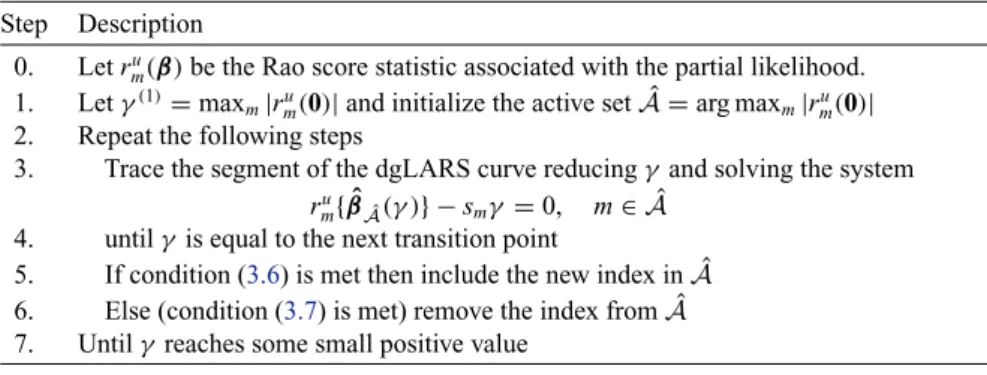
inAˆotherwise condition (3.7) occurs and an index is removed fromA. In the first case, the previous systemˆ is updated adding a new nonlinear equation while, in the second case, a nonlinear equation is removed. The curve is traced as previously described until parameterγ is equal to some fixed value that can be zero, if the sample size is large enough, or some positive value if we are working in a high-dimensional setting, i.e., the number of predictors is larger than the sample size. Table1reports the pseudocode of the developed algorithm to compute the dgLARS curve for a relative regression model. From a computational point of view, the entire dgLARS curve can be computed using the predictor–corrector algorithm proposed inAugugliaroand others(2013); for more details about this algorithm the interested reader is referred toAugugliaroand others(2014,2016) orPaziraand others(2018). The latter extend the dgLARS method to GLM based on the exponential dispersion family proposing an improved predictor–corrector algorithm.
3.3. Tuning parameter selection: derivation of the Generalized Information Criterion
In the previous sections, we have seen how to extend the dgLARS method to relative regression models and how to construct the corresponding path of solutions. In this section, we address the problem of how to select the optimal point of such curve; in other words, the problem of finding the optimalγ-value. The behavior of any penalized estimator, such as Lasso or SCAD, is closely related to the way of selecting
Table 1.Pseudocode of the dgLARS algorithm for a relative risk regression model
Step Description 0. Letru
m(β)be the Rao score statistic associated with the partial likelihood. 1. Letγ(1)=max
m|rum(0)|and initialize the active setAˆ=arg maxm|rmu(0)| 2. Repeat the following steps
3. Trace the segment of the dgLARS curve reducingγand solving the system rum{βˆ
ˆ
A(γ )} −smγ=0, m∈ ˆA 4. untilγis equal to the next transition point
5. If condition (3.6) is met then include the new index inAˆ 6. Else (condition (3.7) is met) remove the index fromAˆ 7. Untilγreaches some small positive value
the value of the tuning parameter because it controls the trade-off between bias and variance. Usually, the tuning parameter is selected using a suitable information criterion which can be written as:
model fit+Cn× model complexity, (3.8)
whereCnis some positive sequence that depends only on the sample size. While minus two times the log-likelihood is commonly used as a measure of model fitting, there are many ways to measure model complexity. For example, this problem is studied for the Lasso estimator inZouand others(2007).
In this article, we propose to select the optimalγ-value of the dgLARS method by using the Generalized Information Criterion (GIC) proposed inKonishi and Kitagawa(1996). For any fixed value of the parameter
γ, dgLARS estimator can be seen as the Z-estimator implicitly defined by the system of estimating equations ∂mp{βˆAˆ(γ )} −smγImm1/2{βˆAˆ(γ )} = i∈D ∂mi,p{βˆAˆ(γ )} −γ smImm1/2{βˆAˆ(γ )} |D| = i∈D φi,m{βˆAˆ(γ )} =0, m∈ ˆA, wherep(β) =
i∈Di,p(β)is the log-partial likelihood function. To the best of our knowledge, the approach developed inKonishi and Kitagawa(1996) is the only one providing a rigorous definition of model complexity for Z-estimators. Using definition (3.8), the GIC measure for the dgLARS estimator applied to the relative risk regression model is defined as
GIC(Cn)= −2p{βˆ(γ )} +Cntr
R−1{βˆ(γ )}Q{βˆ(γ )}
, (3.9)
whereR{βˆ(γ )}andQ{βˆ(γ )}are| ˆA| × | ˆA|matrices with generic elements
Rmn{βˆ(γ )} = − 1 |D| i∈D ∂φi,m{βˆ(γ )} ∂βn and Qmn{βˆ(γ )} = 1 |D| i∈Dφi,m{βˆ(γ )}∂ni,p{βˆ(γ )},
respectively.
For the case of the Cox regression model, i.e.,ψ{x(t);β} = exp{βx(t)}, the log-partial likelihood function is equal to p(β)= i∈D ⎡ ⎣βxi(t i)−log j∈R(ti) exp{βxj(ti)} ⎤ ⎦. (3.10)
As shown inCox(1972), we know that
∂mp(β)= i∈D {xim(ti)−Ai,m(β)}, (3.11) whereAi,m(β)= j∈R(ti)exp{β xj(t i)}xim(ti)/ j∈R(ti)exp{β xj(t
i)}, and themth element of the Fisher information matrix is equal to
Imn(β)= − ∂2 p(β) ∂βm∂βn = i∈D ∂Ai,m(β) ∂βn = i∈D
{Ci,mn(β)−Ai,m(β)Ai,n(β)}, (3.12) where Ci,mn(β) = j∈R(ti)exp{β xj(t i)}xim(ti)xin(ti)/ j∈R(ti)exp{β xj(t i)}. Using (3.11) and (3.12), after straightforward algebra we have that
Rmn(β)= 1 |D| Imn(β)+ smγ 2Imm1/2(β) ∂Imm(β) ∂βn , (3.13) where ∂Imm(β) ∂βn = i∈D
Ci,mmn(β)−Ci,mm(β)Ai,n(β)−2Ai,m(β)
∂Ai,m(β) ∂βn , andCi,mmn(β)= j∈R(ti)exp{β xj(t i)}x2im(ti)xin(ti)/ j∈R(ti)exp{β xj(t i)}. Finally, Qmn(β)= 1 |D| i∈D ∂mi,p(β)∂ni,p(β)− smγImm1/2(β)∂np(β) |D| . (3.14)
The information criterion (3.9) is obtained evaluating the expressions (3.10), (3.13), and (3.14) at the point ˆ
βAˆ(γ ).
4. SIMULATION STUDY
In this section, we compare the method introduced in Section3.2with three popular algorithms: the coor-dinate descent method developed bySimonand others(2011), named CoxNet, the predictor–corrector developed byPark and Hastie(2007), named CoxPath, and the gradient ascent algorithm proposed by Goe-man(2010), named CoxPen. These algorithms are implemented in theRpackagesglmnet,glmpath,
andpenalized, respectively. Given the fact that these methods have only been implemented only for
Cox regression model, our comparison will focus on this kind of relative risk regression model. In the following of this section, dgLARS method applied to the Cox regression model is referred to as thedgCox
model.
4.1. Comparison with other methods: the scale invariance
Letp(β)be the partial log-likelihood function, then the Lasso estimator is defined as solution of the problem max β p(β)−γ p m=1 |βm|, (4.1)
whereγis a non-negative tuning parameter used to control the amount of sparsity in the resulting estimates; whenγis large some elements of the resulting Lasso estimates will be exactly equal to zero whereas when
γgoes to zero the sparsity is reduced since more predictors will be included in the estimated model. To better understand how the scale of the predictors influences the behavior of the Lasso estimator letxim =cmzim, with n i=1zim =0 and n i=1z 2
im= 1, then problem (4.1) is equivalent to the following reparameterized Lasso problem
max ζ p(ζ)−
p
m=1
γm|ζm|, (4.2)
whereζm = cmβm and γm = γ /cm is a tuning parameter specific for the mth regression coefficient. Problem (4.2) reveals that the scale factor of each predictor, i.e., the quantitycm, influences the behavior of the Lasso estimator by changing the scale of the tuning parameter. For example, an increase of the factorcmimplies a reduction of the parameterγmconsequently, with high probability, themth predictor will included in the estimated model even if it does not influence the true relative risk function. The previous example shows that the ability of the Lasso estimator to select a set of predictors is not invariant under scale transformation of the predictors. dgLARS implicitly overcomes this theoretical limitation by using the Rao score test statistic and characterization (3.3) for variable selection. As consequence of the elementary properties of the Rao score test statistic, the variable selection property of the dgLARS method is scale invariant. For more details the reader is referred toAugugliaroand others(2016).
To study the practical effect, we perform a simulation study involving a Cox regression model where the survival timetiis drawn from an exponential distribution with parameterλi = exp(βxi)andxiis sampled from ap-variate normal distribution N(0,I), whereIdenotes the identity matrix. The censorship is randomly assigned to the survival times with probabilityπ =0.5. In our study, the sample sizenis fixed to 100,pis fixed to 10 andβmis equal to 0.5, form=1, 2, 3; the remaining 7 regression coefficients are 0.
To evaluate how the variable selection behavior is related to the scale of the predictors, we rescale in each simulation run the predictors with no effect to have Euclidean norm equal tok. In our study
k varies from 1 to 4. Then we compute the path associated to dgCox, CoxNet, CoxPath, and CoxPen methods, respectively. For each point of a given path, denoted asβˆ(γ ), we compute the False Positive Rate [FPR(γ )], i.e., the ratio between the number of false predictors selected by βˆ(γ ) and the total number of false predictors, and the True Positive Rate [TPR(γ )], i.e., the ratio between the number of true predictors selected byβˆ(γ )and the total number of true predictors. These quantities are used to compute the Receiver Operating Characteristic (ROC) curve and the corresponding Area Under the Curve (AUC). Finally, the four average AUCs are computed and studied as function of the Euclidean norm of the predictors with regression coefficient equal to zero. Figure1 clearly confirms what we previously discussed, i.e., the variable selection behavior of the dgLARS method is scale invariant while the ability of the Lasso estimator to select the true model decreases as thekis increasing.
Fig. 1. Average area under the ROC curves seen as function of the Euclidean norm of the predictors with regression coefficient equal to zero.
4.2. Global comparison with other path-estimation methods
We simulated 100 datasets from a Cox regression model where the survival timesti(i=1,. . .,n) follow an exponential distributions with parameterλi=exp(βxi), andxiis sampled from ap-variate normal distribution N(0,); the entries ofare fixed to corr(Xm,Xn)=ρ|m−n|withρ ∈ {0.3, 0.9}. The censorship is randomly assigned to the survival times with probabilityπ ∈ {0.2, 0.4}. The number of predictors is equal to 100 and the sample size is equal to 50 and 150. The first value is used to evaluate the behavior of the methods is a high-dimensional setting. Finally, we setβm =0.2 form=1,. . .,s, wheres∈ {5, 10}; the remaining parameters are set equal to zero.
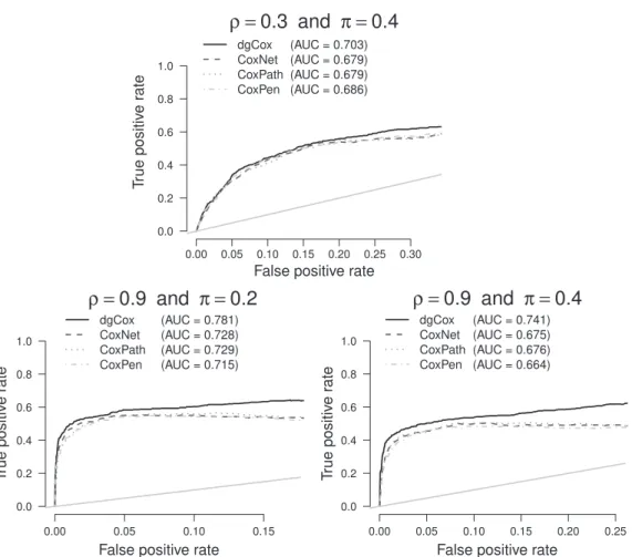
To remove the effects coming from the information measure used to select the optimal point of each path of solutions, we evaluated the global behavior of the paths by considering the ROC curves, which were computed as described in Section4.1. For the sake of brevity, in Fig.2we show only the results for the simulation study with sample size equal to 50; the complete list of figures is reported in the supplementary materialavailable atBiostatisticsonline. In this figure, we compare the ROC curves of our method with the three implementations of the lasso regularized Cox proportional hazards regression across six scenarios. In scenarios whereρ=0.3, CoxNet, CoxPath, and CoxPen exhibit a similar performance, having overlapping curves for both levels of censoring, whereas dgCox method appears to be consistently better with the largest AUC. A similar performance of the methods has been also observed for the other combinations of theρandπvalues. In scenarios where the correlation among neighboring predictors is high, i.e.,ρ =0.9, the dgCox method is clearly the superior approach for all levels of censoring. As shown in the figures reported in thesupplementary materialavailable atBiostatisticsonline, a similar result is obtained when we increase the sample size.
4.3. Tuning parameter selection comparisons
As seen in Section3.3, the behavior of any penalized method is closely related to the information criterion used to select the optimal point of the path of solutions. The simulation study reported in this section is intended to examine the finite sample performance of a number of model information criteria applied to the
Fig. 2. Results from the simulation study withs= 5 and sample size equal to 50; for each scenario, we show the averaged ROC curve for dgCox, CoxNet, CoxPath, and CoxPen algorithm. The average AUC is also reported. The 45◦diagonal is also included in the plots.
dgCox model. The measures that we considered in our study are the Akaike Information Criterion (AIC), the Bayesian Information Criterion (BIC), the GIC proposed inFan and Tang(2013) (FAN13), which uses
Cn=log(log|D|)logpand complexity term| ˆA(γ )|, and two possible versions of the GIC measure (3.9), withCn=2, as originally proposed, andCn=log|D|, imitating the BIC. All the considered criteria are based on using the partial log-likelihood as measure of model fit.
The simulation study in this section follows a similar data generation mechanism as discussed in Section 4.2; we fix the censoring probabilityπ = 0.2, the sample sizesn ∈ {50, 200}andp∈ {50, 100, 1000}. This scenario also covers the high-dimensional setting. The level of sparsity in the true model varies: for the firstd = {2, 8, 32}predictors we fix the coefficients to 0.5, whereas the remaining coefficients are set to zero. The same correlation structureas in Section4.2is considered withρ=0.9. For each scenario, we simulate 500 data sets and let the dgCox method computes the entire path of solutions. Then, we use the considered information criteria to select the optimalγ-value.
For the sake of brevity, in Table2we report only the results of the simulation study with sample size equal ton=50; the remaining results are reported in thesupplementary materialavailable atBiostatistics
online. To evaluate the behavior of the considered criteria we use the median number of variables included
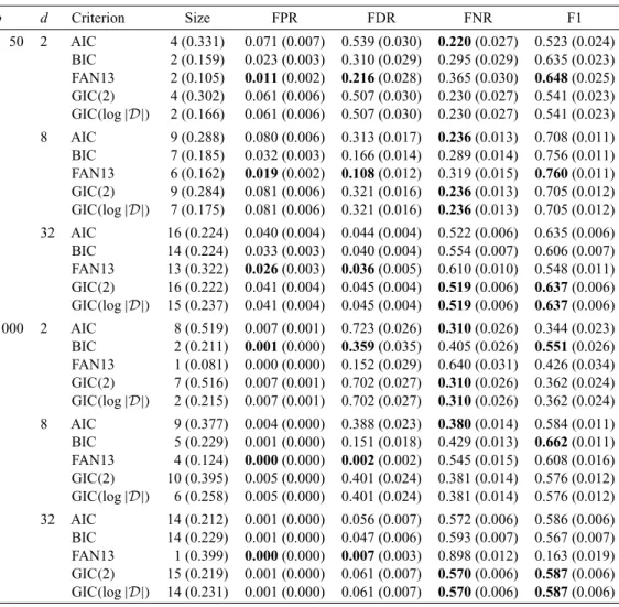
Table 2.Results from the simulation studies when n=50; for each scenario we report the median number of variables included in the final model (Size), the mean of the false positive rate (FPR), the false discovery rate (FDR), the false negative rate (FNR), and F1-score (F1). Standard errors are in parentheses. Bold values identify the best information criterion for each scenario
p d Criterion Size FPR FDR FNR F1 50 2 AIC 4 (0.331) 0.071 (0.007) 0.539 (0.030) 0.220(0.027) 0.523 (0.024) BIC 2 (0.159) 0.023 (0.003) 0.310 (0.029) 0.295 (0.029) 0.635 (0.023) FAN13 2 (0.105) 0.011(0.002) 0.216(0.028) 0.365 (0.030) 0.648(0.025) GIC(2) 4 (0.302) 0.061 (0.006) 0.507 (0.030) 0.230 (0.027) 0.541 (0.023) GIC(log|D|) 2 (0.166) 0.061 (0.006) 0.507 (0.030) 0.230 (0.027) 0.541 (0.023) 8 AIC 9 (0.288) 0.080 (0.006) 0.313 (0.017) 0.236(0.013) 0.708 (0.011) BIC 7 (0.185) 0.032 (0.003) 0.166 (0.014) 0.289 (0.014) 0.756 (0.011) FAN13 6 (0.162) 0.019(0.002) 0.108(0.012) 0.319 (0.015) 0.760(0.011) GIC(2) 9 (0.284) 0.081 (0.006) 0.321 (0.016) 0.236(0.013) 0.705 (0.012) GIC(log|D|) 7 (0.175) 0.081 (0.006) 0.321 (0.016) 0.236(0.013) 0.705 (0.012) 32 AIC 16 (0.224) 0.040 (0.004) 0.044 (0.004) 0.522 (0.006) 0.635 (0.006) BIC 14 (0.224) 0.033 (0.003) 0.040 (0.004) 0.554 (0.007) 0.606 (0.007) FAN13 13 (0.322) 0.026(0.003) 0.036(0.005) 0.610 (0.010) 0.548 (0.011) GIC(2) 16 (0.222) 0.041 (0.004) 0.045 (0.004) 0.519(0.006) 0.637(0.006) GIC(log|D|) 15 (0.237) 0.041 (0.004) 0.045 (0.004) 0.519(0.006) 0.637(0.006) 1000 2 AIC 8 (0.519) 0.007 (0.001) 0.723 (0.026) 0.310(0.026) 0.344 (0.023) BIC 2 (0.211) 0.001(0.000) 0.359(0.035) 0.405 (0.026) 0.551(0.026) FAN13 1 (0.081) 0.000 (0.000) 0.152 (0.029) 0.640 (0.031) 0.426 (0.034) GIC(2) 7 (0.516) 0.007 (0.001) 0.702 (0.027) 0.310(0.026) 0.362 (0.024) GIC(log|D|) 2 (0.215) 0.007 (0.001) 0.702 (0.027) 0.310(0.026) 0.362 (0.024) 8 AIC 9 (0.377) 0.004 (0.000) 0.388 (0.023) 0.380(0.014) 0.584 (0.011) BIC 5 (0.229) 0.001 (0.000) 0.151 (0.018) 0.429 (0.013) 0.662(0.011) FAN13 4 (0.124) 0.000(0.000) 0.002(0.002) 0.545 (0.015) 0.608 (0.016) GIC(2) 10 (0.395) 0.005 (0.000) 0.401 (0.024) 0.381 (0.014) 0.576 (0.012) GIC(log|D|) 6 (0.258) 0.005 (0.000) 0.401 (0.024) 0.381 (0.014) 0.576 (0.012) 32 AIC 14 (0.212) 0.001 (0.000) 0.056 (0.007) 0.572 (0.006) 0.586 (0.006) BIC 14 (0.229) 0.001 (0.000) 0.047 (0.006) 0.593 (0.007) 0.567 (0.007) FAN13 1 (0.399) 0.000(0.000) 0.007(0.003) 0.898 (0.012) 0.163 (0.019) GIC(2) 15 (0.219) 0.001 (0.000) 0.061 (0.007) 0.570(0.006) 0.587(0.006) GIC(log|D|) 14 (0.231) 0.001 (0.000) 0.061 (0.007) 0.570(0.006) 0.587(0.006)
in the final model (Size), the average false positive rate (FPR), the false discovery rate (FDR), the false negative rate (FNR), and F1-score (F1) to investigate the performance of the model selection criteria in identifying the true model. The results in Table2show that there is a clear trade-off between FNR and FPR. Therefore, it can be more informative to compare a summary measure, such as the F1-score. Summarizing, we found that in very sparse contexts, i.e., the true number of effects is small (d p), FAN13 performs well in terms of F1-score. The two GIC measures perform well whendincreases, slightly beating FAN13. The traditional AIC and BIC criteria do not perform as well: the reason could be that the penalized partial likelihood setting violate the usual assumptions for these methods in that model fit should be measured as a maximum likelihood, not as a penalized partial likelihood.
5. FINDING GENETIC SIGNATURES IN CANCER SURVIVAL
In this section, we test the predictive power of proposed method in four recent studies. In particular, we focus on the identification of genes involved in the regulation of colon cancer (Lobodaand others, 2011), prostate cancer (Rossand others,2012), ovarian cancer (Gilletand others,2012), and skin cancer (Jönssonand others,2010). The set-up of the four studies was similar. In the patient a cancer was detected and treated. When treatment was complete a follow-up started. In all cases, the expression of several genes were measured in the affected tissue together with the survival times of the patients, which may be censored if the patients were alive when they left the study. Although other socio-economical variables, such us age, sex, etc. are available, our analysis only focuses on the impact of the gene expression levels on the patients’ survival.
A table containing a brief description of the four datasets used in this section is reported in the supplementary materialsavailable at Biostatisticsonline. In the four scenarios, the number of predic-torspis larger than the number of patientsn. The dimensionality is especially high in the cases of the colon and skin cancer where the expression of several thousands of genes were measured. In the prostate and ovarian cancers the number of genes is 162 and 306, which will also help us to study the performance of the dgLARS method when the number of variables is just a few orders of magnitude larger than the number of observations.
In genomics, it is common to assume that just a moderate number of genes affect the phenotype of interest. To identify such genes in this survival context, we estimate a Cox regression model using the dgLARS method described in Section3. To this end, we randomly select a training sample that contains the 60% of the patients, and we save the remaining data to test the models. We calculate the paths of solutions in the four scenarios and we select the optimal number of components by means of the GIC(log|D|) criterion derived in Section3.3. For the colon, prostate, ovarian, and skin cancer studies we find gene profiles consisting of, respectively, 38, 24, 43, and 23 genes.
In order to illustrate the prediction performance of the dgLARS method, we classify the test patients into a low-risk group and a high-risk groups by splitting the test sample into two subsets of equal size according to the estimated individual predicted excess risk. The first two plots in Fig.3show the Kaplan– Maier survival curves estimates for the low- and high-risk groups together with the original training survival curve for the Colon and Ovarian studies, respectively. To test the groups separation we use the non-parametric Peto & Peto modification of the Gehan–Wilcoxon test (Peto and Peto,1972). For all four studies, the differences between the low- and high-risk groups are significant at the traditional 0.05 significance level.
Alternatively, survival ROC curves (Heagertyand others,2000) can be used to describe how well the selected model is predicting the order of survival of the patients in each of the studies. It can be interpreted as a traditional ROC curve with respect to predicting the survival of the patients. The final two plots in Fig.3show the survival ROC curves for the relatively small ovarian cancer study and the large colon cancer study. The results show that dgCox combined with GIC is better than other sparse survival methods in predicting the survival order. The results for the other two datasets are even more in favor of the dgCox method and are reported in thesupplementary materials available at Biostatis-ticsonline. Both results suggest that the reported gene profiles are predictive for determining survival and it demonstrates the power of dgLARS as a tool in medical analysis for massive gene screening studies.
To gain some biological understanding of the process of cancer regulation we performed an enrichment analysis of the 21 genes that have been found to be relevant in the regulation of the skin cancer. For the sake of brevity the enrichment analysis is reported in thesupplementary materialavailable atBiostatistics
online.
Fig. 3. Top plots: the Kaplan–Meier survival curves for colon and ovarian studies ontrainingdata together with the curves associated to the low- and high-risk groups in thetestsample, showing dgCox’s ability being able to detect low-and high-risk individuals. Bottom plots: survival ROC curves for the same two studies, demonstrating how dgCox combined with GIC has a better predictive performance than other sparse survival methods.
6. CONCLUSIONS
In this article, we have extended the dgLARS method to relative risk regression model using the relationship exiting between the partial likelihood function and a specific GLM. The advantage of this approach is that the estimates are invariant to arbitrary changes in the measurement scales of the predictors. Unlike SCAD or1 sparse regression methods, no prior rescaling of the predictors is therefore needed. The proposed method can be used for a large class of survival models, the so called relative risk models. We have implementations for the Cox proportional hazards model and the excess relative risk model.
In this article, we have also proposed a new information criterion to select the optimal point in the path of solutions defined by applying dgLARS method to a relative risk regression model. As our method
involves shrinkage of the parameters, the issue of the underlying degrees of freedom of the sparse models is a complex one. For this reason, we used the approach developed inKonishi and Kitagawa(1996), which provides a rigorous definition of model complexity for Z-estimators. We showed that the proposed measure works well in a simulation study and is only beaten the method fromFan and Tang(2013) when the true underlying model is extremely sparse.
A software implementation of our method is available on github (https://github.com/LuigiAugugliaro/ dgcox) and can deal with the classicaln>psetting, but also with the high-dimensional setting, such as, for example, a skin cancer study withp=30 807 predictors andn=54 observations. We have considered four recent cancer survival studies, where we look for a genetic “survival signature.” Due to the large number of predictors, the studies are unsuitable for traditional survival regression methods. Instead, the results we find go beyond univariate importance and by means of an enrichment study can be linked to potentially relevant biological explanations.
SUPPLEMENTARY MATERIALS
Supplementary materialis available athttp://biostatistics.oxfordjournals.org.
ACKNOWLEDGMENTS
The authors gratefully acknowledge the editor and two referees, whose comments have improved the quality of this work.
Conflict of Interest: None declared.
FUNDING
The authors have received funding for collaboration through the EU COST Action CA15109 (COSTNET). REFERENCES
AUGUGLIARO, L., MINEO, A. M.ANDWIT, E. C. (2013). Differential geometric least angle regression: a differential geometric approach to sparse generalized linear models.Journal of the Royal Statistical Society Series B75, 471–498.
AUGUGLIARO, L., MINEO, A. M.ANDWIT, E. C. (2014). dglars: an R package to estimate sparse generalized linear models.Journal of Statistical Software59, 1–40.
AUGUGLIARO, L., MINEO, A. M.ANDWIT, E. C. (2016). A differential geometric approach to generalized linear models with grouped predictors.Biometrika103, 563–577.
BRESLOW, N. E. (1975). Covariance analysis of censored survival data.Biometrics30, 89–99.
COX, D. R. (1972). Regression models and life-tables.Journal of the Royal Statistical Society Series B34, 187–220. COX, D. R. (1975). Partial likelihood.Biometrika62, 269–276.
COX, D. R. (1981). Discussion of paper by D. Oakse entitled “Survival times: aspects of partial likelihood”. International Statistical Review49, 258.
COX, D. R.ANDOAKES, D. (1984).Analysis of Survival Data. Monographs on Statistics and Applied Probability. London: Chapman and Hall.
EFRON, B. (1977). The efficiency of Cox’s likelihood function for censored data.Journal of the American Statistical Association72, 557–565.
EFRON, B., HASTIE, T., JOHNSTONE, I.ANDTIBSHIRANI, R. (2004). Least angle regression.The Annals of Statistics32, 407–499.
FAN, J.ANDLI, R. (2001). Variable selection via nonconcave penalized likelihood and its oracle properties.Journal of the American Statistical Association96, 1348–1360.
FAN, Y.ANDTANG, C. Y. (2013). Tuning parameter selection in high dimensional penalized likelihood.Journal of the Royal Statistical Society Series B75, 531–552.
GILLET, J. P., CALCAGNO, A. M., VARMA, S., DAVIDSON, B., ELSTRAND, M. B., GANAPATHI, R., KAMAT, A. A., SOOD, A. K., AMBUDKAR, S. V., SEIDEN, M. V.and others. (2012). Multidrug resistance-linked gene signature predicts overall survival of patients with primary ovarian serous carcinoma.Clinical Cancer Research18, 3197–3206. GOEMAN, J. J. (2010). L1 penalized estimation in the Cox proportional hazards model.Biometrical Journal52, 70–84. GUI, J.ANDLI, H. (2005). Penalized Cox regression analysis in the high-dimensional and low-sample size settings,
with applications to microarray gene expression data.Bioinformatics21, 3001–3008.
HEAGERTY, P. J., LUMLEY, T.ANDPEPE, M. S. (2000). Time-dependent ROC curves for censored survival data and a diagnostic marker.Biometrics56, 337–344.
JÖNSSON, G., BUSCH, C., KNAPPSKOG, S., GEISLER, J., MILETIC, H., RINGNÉR, LILLEHAUG, J. R., BORG, A.AND
LØNNING, P. E. (2010). Gene expression profiling-based identification of molecular subtypes in stage IV melanomas with different clinical outcome.Clinical Cancer Research16, 3356–3367.
KALBFLEISCH, J. D.ANDPRENTICE, R. L. (2002).The Statistical Analysis of Failure Time Data, Wiley Series in Probability and Statistics. Hoboken, New Jersey: John Wiley & Sons, Inc.
KONISHI, S.ANDKITAGAWA, G. (1996). Generalised information criteria in model selection.Biometrika83, 875–890. LOBODA, A., NEBOZHYN, M. V., WATTERS, J. W., BUSER, C. A., SHAW, P. M., Huang, P. S., L. Van’t Veer, R. A. Tollenaar, Jackson, D. B., Agrawal, D.and others. (2011). EMT is the dominant program in human colon cancer.BMC Medical Genomics,4, 9.
MCCULLAGH, P.ANDNELDER, J. A. (1989).Generalized Linear Models, 2nd edition. London: Chapman & Hall. MOOLGAVKAR, S. H.ANDVENZON, D. J. (1987). Confidence regions in curved exponential families: application to
matched case-control and survival studies with general relative risk function.The Annals of Statistics15, 346–359. OAKES, D. (1981). Survival times: aspects of partial likelihood.International Statistical Review49, 235–252. PARK, M. Y.ANDHASTIE, T. (2007). L1-regularization path algorithm for generalized linear models.Journal of the
Royal Statistical Society Series B69, 659–677.
PAZIRA, H., AUGUGLIARO, L.ANDWIT, E. C. (2018). Extended differential geometric LARS for high-dimensional GLMs with general dispersion parameter.Statistics and Computing28, 753–774.
PETO, R.ANDPETO, J. (1972). Asymptotically efficient rank invariant test procedures.Journal of the Royal Statistical Society Series A135, 185–207.
PRENTICE, R. L.ANDBRESLOW, N. E. (1978). Retrospective studies and failure time models.Biometrika65, 153–158. PRENTICE, R. L.ANDMASON, M. W. (1996). On the application of linear relative risk regression models.Biometrics42,
109–120.
PRENTICE, R. L., YOSHIMOTO, Y.ANDMASON, M. (1983). Relationship of cigarette smoking and radiation exposure to cancer mortality in Hiroshima and Nagasaki.Journal of National Cancer Institute70, 611–622.
RAO, C. R. (1949). On the distance between two populations.Sankhy¯a9, 246–248.
RIPPE, R. C. A., MEULMAN, J. J.ANDEILERS, P. H. C. (2012). Visualization of genomic changes by segmented smoothing using anL0penalty.PLoS One7, e38230.
ROSS, R. W., GALSKY, M. D., SCHER, H. I., MAGIDSON, J., WASSMANN, K., LEE, G. S. M., KATZ, L., SUBUDHI, S. K., ANAND, A., FLEISHER, M., KANTOFF, P. W.and others. (2012). A whole-blood RNA transcript-based prognostic model in men with castration-resistant prostate cancer: a prospective study.The Lancet Oncology13, 1105–1113.
SIMON, N., FRIEDMAN, J. H., HASTIE, T.ANDTIBSHIRANI, R. (2011). Regularization paths for Cox’s proportional hazards model via coordinate descent.Journal of Statistical Software39, 1–13.
SOHN, I., KIM, J., JUNG, S. H. AND Park, C. (2009). Gradient lasso for Cox proportional hazards model. Bioinformatics25, 1775–1781.
THOMAS, D. C. (1977). Addendum to the paper by Liddell, McDonald, Thomas and Cunliffe.Journal of the Royal Statistical Society Series A140, 483–485.
THOMAS, D. C. (1981). General relative-risk models for survival time and matched case-control analysis. Biometrics37, 673–686.
TIBSHIRANI, R. (1996). Regression shrinkage and selection via the lasso.Journal of the Royal Statistical Society Series B58, 267–288.
TIBSHIRANI, R. (1997). The lasso method for variable selection in the Cox model.Statistics in medicine16, 385–395. ZOU, H.ANDHASTIE, T. (2005). Regularization and variable selection via the elastic net.Journal of the Royal Statistical
Society Series B, 301–320.
ZOU, H., HASTIE, T.ANDTIBSHIRANI, R. (2007). On the “degrees of freedom” of the LASSO.TheAnnals of Statistics35, 2173–2192.
[Received May 13, 2017; revised September 20, 2018; accepted for publication September 24, 2018]