A new method based on Type-2 fuzzy neural network for accurate wind power forecasting under uncertain data

Elsevier required licence: © 2018. This manuscript version is made available under the CC-BY-NC-ND 4.0 license

http://creativecommons.org/licenses/by-nc-nd/4.0/

1

A New Method Based on Type-2 Fuzzy Neural Network

1

for Accurate Wind Power Forecasting under Uncertain

2

Data

3

4

Amir Sharifian*,M. Jabbari Ghadi#, Sahand Ghavidel#, Li Li#, Jiangfeng Zhang#

5

*Department of Electrical Engineering, Ahrar Institute of Technology and Higher Education, P.O.Box

6

41931-63584, Rasht, Iran.

7

#

Faculty of Engineering and Information Technology, University of Technology Sydney, PO Box 123,

8

Broadway, NSW 2007, Australia

9

*_{Email: [email protected]}

₁₀

#

Email: {mojtaba.jabbarighadi, sahand.ghavideljirsaraie}@student.uts.edu.au, {li.li,

11

Jiangfeng.Zhang}@uts.edu.au

12

13

Abstract

14

Nowadays, due to some environmental restrictions and decrease of fossil fuel sources, renewable energy

15

sources and specifically wind power plants have a major part of energy generation in the industrial

16

countries. To this end, the accurate forecasting of wind power is considered as an important and influential

17

factor for the management and planning of power systems.

18

In this paper, a novel intelligent method is proposed to provide an accurate forecast of the medium-term

19

and long-term wind power by using the uncertain data from an online supervisory control and data

20

acquisition

(

SCADA) system and the numerical weather prediction (NWP). This new method is based on

21

the particle swarm optimization (PSO) algorithm and applied to train the Type-2 fuzzy neural network

22

(T2FNN) which is called T2FNN-PSO. The presented method combines both of fuzzy system’s expert

23

knowledge and the neural network’s learning capability for accurate forecasting of the wind power. In

24

addition, the T2FNN-PSO can appropriately handle the uncertainties associated with the measured

25

2

parameters from SCADA system, the numerical weather prediction and measuring tools.

1

The proposed method is applied on a case study of a real wind farm. The obtained simulation results

2

validate effectiveness and applicability of the proposed method for a practical solution to an accurate wind

3

power forecasting in a power system control center.

4

Index Terms

5

Type-2 fuzzy neural network, PSO algorithm, Medium-term and long-term wind power forecasting,

6

uncertain information.

7

*Corresponding Author: Amir Sharifian; Postal address: Department of Electrical Engineering, Ahrar

8

Institute of Technology and Higher Education, P.O. Box 41931-63584, Rasht, Iran.

9

Phone: +98-13-33424373, Fax: +98-13-33424256, E-mail: [email protected]

10

11

1. I

NTRODUCTION

12

Nowadays, the utilization of thermal power plants has faced lots of limitations due to some

13

environmental restrictions and deep concerns about the air pollution as well as depletion of fossil fuel

14

resources. That is why in recent years, the development of renewable energy resources particularly wind

15

power plants has played a key role in the electricity energy production in many counties [1]. Wind power

16

plants have many advantages because of their relatively little impact to environment, lack of pollution, and

17

being renewable.

18

However, one major problem about high penetration of wind power plants into power grids is the

19

uncertainties associated with the forecasting of wind power in different time horizons. Considering high

20

fluctuations of these parameters during different hours, accurate forecasting of wind power is considerably

21

complicated. Based on power system operation requirements, the forecasting can be divided into three time

22

horizons: short-term (few seconds to 30 min), medium-term (30 min to 24 h) and long-term (1 to 7 days).

23

The wind power forecasting in different time periods has an important role in the planning, management

24

and operation of power systems [1].

25

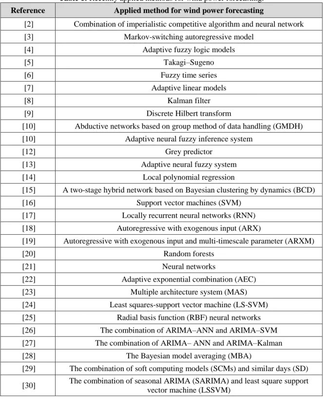
Recently, a large number of methods have been presented to forecast the wind power. These methods

26

are divided into three parts including physical forecasting methods, statistical forecasting methods and

27

3

combined forecasting methods. A comprehensive explanation of these methods is provided in [1], where it

1

is mentioned that advantage of each of these presented methods depends on the wind farm conditions.

2

However, among these methods, combined forecasting methods are more useful and also have higher

3

accuracy than others. In [2], the authors present a method for medium-term and long-term output power

4

forecasting of wind turbines as a function of measured parameters by the SCADA system, and the

5

forecasted parameters are obtained from the numerical weather prediction (NWP) (i.e. air pressure,

6

humidity, wind speed and direction, and temperature). The recently applied methods for wind power

7

forecasting are summarized in Table 1.

8

As it can be seen in Table 1, no research has been done for wind power forecast which considers

9

simultaneously uncertainties associated with measured parameters from the SCADA system, the forecasted

10

parameters and measuring tools.

11

An innovative method based on the artificial intelligence is employed for solving many different

12

problems in power systems instead of performing heavy and time-consuming calculations. These

13

techniques are more practical and suitable for online applications. One of the most popular and practical

14

artificial intelligence techniques is the Type-2 fuzzy neural network (T2FNN) which combines the

15

linguistic interception feature of the Type-2 fuzzy set and the learning capacity of the neural network

16

[31,34-35]. Moreover, this network can handle the uncertainty associated with input parameters.

17

In this paper, a novel intelligent method based on T2FNN estimation and the particle swarm

18

optimization (PSO) algorithm is proposed for the medium-term and the long-term wind power forecasting

19

under the uncertain data. The presented approach combines the Fuzzy system’s export knowledge and

20

neural network’s learning capability to forecast the wind power, thus termed T2FNN-PSO. In addition, the

21

T2FNN-PSO can appropriately handle the uncertainties that are associated with input parameters and

22

measuring tools. The performance of proposed method is evaluated by using the obtained data from a real

23

wind farm. This method is implemented for two periods of time (medium-term and long-term). The

24

simulation results demonstrate that the suggested method is accurate and practical for wind power

25

forecasting.

26

4

Table 1: Recently applied methods for wind power forecasting. Reference Applied method for wind power forecasting

[2] Combination of imperialistic competitive algorithm and neural network [3] Markov-switching autoregressive model

[4] Adaptive fuzzy logic models

[5] Takagi–Sugeno

[6] Fuzzy time series

[7] Adaptive linear models

[8] Kalman filter

[9] Discrete Hilbert transform

[10] Abductive networks based on group method of data handling (GMDH) [10] Adaptive neural fuzzy inference system

[12] Grey predictor

[13] Adaptive neural fuzzy system

[14] Local polynomial regression

[15] A two-stage hybrid network based on Bayesian clustering by dynamics (BCD)

[16] Support vector machines (SVM)

[17] Locally recurrent neural networks (RNN) [18] Autoregressive with exogenous input (ARX)

[19] Autoregressive with exogenous input and multi-timescale parameter (ARXM)

[20] Random forests

[21] Neural networks

[22] Adaptive exponential combination (AEC) [23] Multiple architecture system (MAS) [24] Least squares-support vector machine (LS-SVM) [25] Radial basis function (RBF) neural networks [26] The combination of ARIMA–ANN and ARIMA–SVM [27] The combination of ARIMA– ANN and ARIMA–Kalman [28] The Bayesian model averaging (MBA)

[29] The combination of soft computing models (SCMs) and similar days (SD) [30] The combination of seasonal ARIMA (SARIMA) and least square support

vector machine (LSSVM)

1

In summary, the contributions of this paper can be listed as follows:

2

1- To present a novel intelligent method based on the T2FNN estimation and PSO algorithm for

3

accurate wind power forecasting.

4

2- To effectively handle the uncertainty of measured parameters of the SCADA system and the

5

forecasted parameters from NWP and measuring tools by T2FNN.

6

5

3- To apply a new training method based on PSO algorithm for tuning parameters of the T2FNN.

1

The rest of paper is presented as follows:

2

Section 2 describes the methodology of the T2FNN-PSO for the wind power forecasting. Section 3

3

introduces the structure and training approach of the proposed T2FNN-PSO. Section 4 explains simulation

4

results and the discussion; and finally, the conclusion is presented in Section 5.

5

2.

M

ETHODOLOGY FOR WIND POWER FORECASTING

6

Environmental restrictions besides the increase of fossil fuels price have encouraged power system

7

operators to employ renewable energies and specifically wind power during the last decade. On the other

8

hand, an accurate wind power forecasting can play an influential role in both of the operation and planning

9

of power systems. According to [2], the power forecasting of a wind farm can be obtained based on the

10

data obtained from the SCADA system and the NWP (i.e. air pressure, humidity, wind speed and direction,

11

temperature). Duo to the chaotic feature of these parameters, the accurate forecasting of generating power

12

of a wind turbine in a practical case is a complex obligation. In addition, this subject becomes more

13

complex when the uncertainties with these parameters are considered in the system model. In our previous

14

work [31], we compared the efficiency and performance of the proposed T2FNN with a multi-layer

15

perceptron (MLP) and radial basis function (RBF) neural networks. The obtained results show a better

16

performance of the proposed T2FNN in terms of accuracy, handling uncertainty and computational costs.

17

Therefore, in this paper, the proposed T2FNN is used to forecast the generated wind power.

18

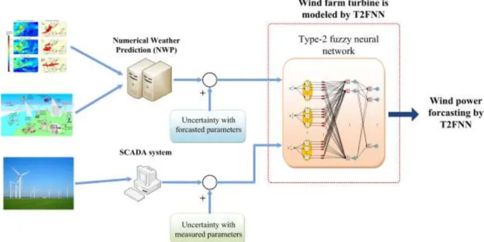
In this section, details of our new method based on T2FNN-PSO estimation for forecasting of the

19

generated wind power are designated. The structure of the proposed approach is illustrated in Fig. 1. As it

20

can be seen, each turbine in the wind farm is modeled by using the T2FNN-PSO. The T2FNN-PSO is able

21

to estimate the value of the wind power by using its input parameter. The values of measured parameters by

22

the SCADA system and the NWP are selected as inputs of T2FNN [2]. It’s obvious that due to the natural

23

noise and uncertainties with measured and forecasting tools, the obtained values from the NWP and the

24

SCADA system are associated with uncertainties. Therefore, it is necessary to apply a T2FNN-PSO in

25

6

Figure 1: Block Diagram of the proposed method based on T2FNN-PSO.

In order to reach a promising estimate for the value of wind power, it is essential to utilize a correct and

1

accurate training algorithm for tuning T2FNN parameters. In this paper, a new method based on the PSO

2

algorithm is applied to train the T2FNN.

3

2.1.

N

UMERICAL WIND PREDICTION MODEL

4

Nowadays, the weather forecast has a non-negligible impact on the medium-term (i.e. less than 1

5

hour~24 hours) and long-term (i.e. more than 24 hours) wind power forecasting. NWP focuses on

6

collecting current weather observations and processing these data with supercomputers for forecasting the

7

future status of weather. Therefore, having the accurate status of the current weather is as vital as the

8

numerical models processing the data. Current weather observations serve as input to the numerical models

9

through a process known as data assimilation to produce the outputs of temperature, wind speed, and

10

hundreds of other meteorological elements from the oceans to the top of the atmosphere. The NWP models

11

use physical conversion of energy equations and this allows more realistic downscaling of the data. In fact,

12

high-resolution NWP plays the key role for the wind power forecast [2].

13

Recently, based on available computational systems, NWP models become more popular in many wind

14

power estimation studies; where several NWP models such as the weather research and forecasting (WRF),

15

conductor-like screening model (COSMO), fifth-generation Penn State/NCAR Mesoscale model (MM5),

16

7

and RAMS (i.e. reliability, availability, maintainability, and safety) are applied [1]. Also, various methods

1

of extrapolation such as the logarithmic law and the wind shear power law have been proposed by other

2

researchers to provide appropriate wind information at the height of wind turbine hub (i.e. approximately

3

50 m) using the meteorological data that are gathered at 10 m above the ground (according to the world

4

meteorological organization (WMO) approval) [32]. Needless to say, the usage of extrapolation laws may

5

create considerable deviations in accurate assessment of the wind power forecasting, specifically for long-

6

term timescales [33].

7

In this paper, the forecast data obtained from NWP are utilized as a part of input patterns for the

8

proposed model to forecast wind power in medium-term and long-term timescales. In other words, our

9

model is basically a post-processing neural network model for NWP. The reason lies in the fact that the

10

validated data related to the NWP is only available for a certain period of time ahead, and NWP models do

11

not have high accuracy for long period of times. Therefore, it is not possible to solely rely on the NWP

12

model for the long-term forecast of the wind power. To this end, the SCADA and the historical data play a

13

supplementary role for the NWP data. This structure of input data can improve the accuracy of NWP data

14

for the medium-term power forecasting and also compensate the low efficiency of NWP data during the

15

long-term forecasting.

16

3.

P

ROPOSED

T

YPE

-2

F

UZZY

N

EURAL

N

ETWORK

17

The neural networks have a desirable performance in terms of recognizing input patterns; however they

18

are weak for explaining how they make their decisions. On the other hand, the Type-2 fuzzy systems can

19

explain the rules of complex systems and imprecise information, and can handle the uncertainties

20

associated with system structure, process and measured variables. However, they are unable to

21

automatically acquire the rules which they apply to make these decisions. Therefore, in this paper, these

22

two intelligent techniques are combined to overcome limitations of individual techniques. The combined

23

system is named the T2FNN system. The T2FNN has been applied successfully in many applications

24

including cognitive simulation, process control, medical diagnosis, financial trading, and engineering

25

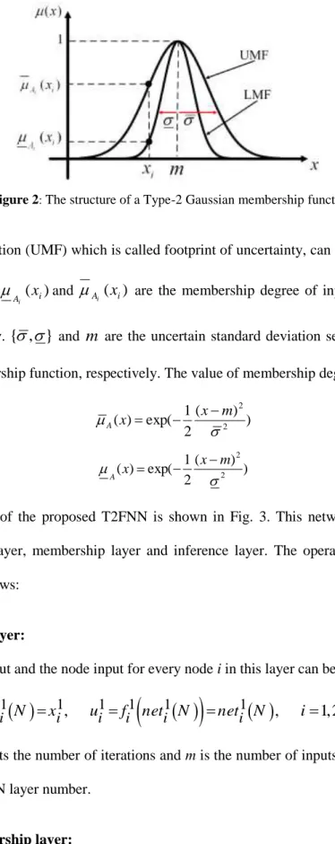
design [31]. The structure of a Type-2 fuzzy Gaussian membership function is shown in Fig. 2.

26

As shown in Fig. 2, the bounded region between lower membership function (LMF) and upper

27

8

Figure 2: The structure of a Type-2 Gaussian membership function.

1

membership function (UMF) which is called footprint of uncertainty, can handle the uncertainty associated

2

with the system. _A (xi) i



and _A

(

x

_i

)

i



are the membership degree of input variable

x

i to the UMF and

3

LMF respectively.

{



,



}

and

m

are the uncertain standard deviation set and the mean of Type-2 fuzzy

4

Gaussian membership function, respectively. The value of membership degree can be written as follows:

5

) ) ( 2 1 exp( ) ( ₂ 2  _A x   xm (1) ) ) ( 2 1 exp( ) ( ₂ 2   x x m A    (2)

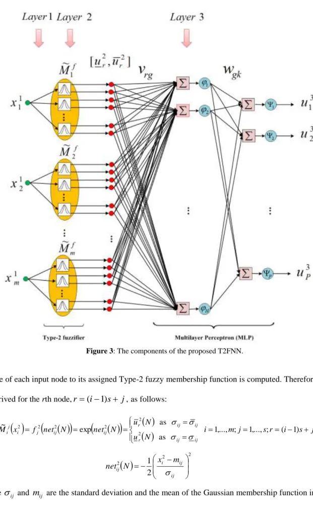
The structure of the proposed T2FNN is shown in Fig. 3. This network is composed of three layers

6

including input layer, membership layer and inference layer. The operation of each layer of T2FNN is

7

described as follows:

8

Layer 1-Input layer:

9

The node output and the node input for every node i in this layer can be described as follows:

10

 



 



 

1 1

_,

1 1 1 1

_,

_1,2,...,

i i i i i i

net

N



x

u



f

net

N



net

N

i



m

₍₃₎

where N represents the number of iterations and m is the number of inputs. The superscripts of all symbols

11

denote the T2FNN layer number.

12

Layer 2- membership layer:

13

In this layer, each node performs a Type-2 fuzzy membership function. Outputs of this layer are

14

fuzzified input nodes which are called linguistic variables. On the other hand, the value of membership

15

9

Figure 3: The components of the proposed T2FNN.

1

degree of each input node to its assigned Type-2 fuzzy membership function is computed. Therefore, it can

2

be derived for the rth node,r (i1)s j,as follows:

3

 



 





 



 

 

N i m j s r i s j u N u N net N net f x M u ij ij r ij ij r ij ij j i j i r                1,..., ; 1,..., ; ( 1) as as exp ~ 2 2 2 2 2 2 2    

 

2 2 2 2 1            ij ij i ij m x N net  (4)

where



_ij and

m

_ij are the standard deviation and the mean of the Gaussian membership function in the jth

4

10

Layer 3- inference layer:

1

This layer is the main part of T2FNN which gives a mapping from input nodes (linguistic variable) to

2

the output (crisp values). The output of kth node can be written as follows:

3

p k u v v w w u r s m r rg g g H g gk k k k , 1, , 2 1 0 1 0 3  _             _  





  





(5)

4

where

u

_r2

,

r



1

,

2

,...,

m



s

is the rth output node in the layer 2. H is the number of neurons in the hidden

5

layer of neural network. The number of neurons in the hidden layer is carefully chosen to provide best

6

results in training phase of the system. Also,



_g and



k are the activation functions for hidden and output

7

layers respectively. v0g and w0kare the bias on the hidden unit g and bias on the output unit k. vrg is the

8

weight connecting the input neuron r to hidden neuron g.wgkis the weight connecting the hidden neuron g

9

to output neuron k.

10

The T2FNN requires the adjustment of its parameters in all the layers such that the desired output can

11

be obtained. These parameters consist of



_ij



{



_ij

,



_ij

}

,

m

_ij,

v

_rgand

w

_gk which are adjusted by using the

12

training algorithm. There are several algorithms such as gradient descent, Levenberg Marquardt and

13

resilient back-propagation for training intelligent systems. Selecting an efficient training algorithm is

14

essential for a desirable performance of the T2FNN. In this paper, a new training method is used based on

15

PSO algorithm to obtain a better training of the T2FNN. Details of the proposed method are described in

16

the next sections.

17

3.1.

S

ETTING OF CONTROLLING PARAMETERS FOR PROPOSED ALGORITHM

18

As aforementioned, the proposed model is composed of two parts: a Type-2 fuzzifier and a MLP neural

19

network. Controlling parameters should be determined for the proposed model are including the number

20

and the type of the fuzzy membership function for input variables and their corresponding average (m) and

21

standard variance (σ) values in case of Type-2 fuzzifier; and weights of neurons in case of the MLP neural

22

network.

23

To this end, the number and the type of the fuzzy membership function (FMF) for input variables are

24

determined based on the knowledge of an expert person. In order to reach optimized values for these

25

11

parameters, considering the small scale of the search space, the trial and error approach and the extensive

1

search have been employed. Authors have tested different types of membership function (e.g. triangular,

2

trapezoidal, piecewise linear, Gaussian, etc.) to reach the best type of FMF. Such the approach has been

3

applied for the number of FMFs. Finally, the value 3 has been determined as the best value for this

4

parameter. It should be mentioned that having more than three membership functions can provide a higher

5

level of accuracy; however, it causes exponential development of the system and subsequently a more

6

complicated network; on the other hand, having values less than three results in loose of accuracy. In fact, a

7

tradeoff has been settled by authors to reach a high quality result with a reasonable computational cost.

8

In case of neurons weight for the structure of the MLP neural network, average (m) and standard

9

variance (σ) values for membership functions, the PSO algorithm is utilized to reach optimized values for

10

these parameters. Obviously, classical methods like gradient descent, Levenberg Marquardt and resilient

11

back-propagation could not offer a high quality performance when the number of variables in each pattern

12

of the input data is large (i.e. 486 for the presented network).

13

14

3.2.

A

PPLICATION OF

PSO

ALGORITHM FOR TRAINING THE PROPOSED

T2FNN

15

PSO is an optimization algorithm that was first developed in 1995 by Eberhart and Kennedy [36]. The

16

results obtained in [37] shows that the training method based on the PSO algorithm has better performance

17

than other training algorithms because of using less c

omputational

time to get higher training accuracy.

18

Therefore, in this paper, the PSO algorithm is applied to train the proposed T2FNN.

19

According to the previous section, the parameters of proposed T2FNN that should be adjusted by using

20

the PSO algorithm in the training phase include



_ij



{



_ij

,



_ij

}

,

m

_ij ,

v

_rgand

w

_gk. The optimization

21

problem proposed in training phase is to search the optimal values of T2FNN parameters by using the PSO

22

algorithm. This results in minimization of the sum of the squared differences between the desired output

23

and actual output. Hence, the objective function can be written as:

24





2 1 ) , , , (



   n i i e i d gk rg ij ij m v w y y J



(6)

where n is the total number of training patterns and i represents the pattern index.

y

_dand yeare the desired

25

output and the actual output, respectively. This objective function needs to be optimized (minimized).

26

12

During the training process, in each of iterations, the value of objective functionis reduced. This iterative

1

process is ended when a given number of iterations are reached or the value of objective function reaches a

2

predetermined value.

3

3.3.

T

RAINING OF

T2FNN

TO PREDICT THE WIND POWER

4

In this section, the training process of proposed T2FNN-PSO is explained. In order for the proposed

5

T2FNN-PSO to be applied for estimating the wind power, a correct training procedure of the network is

6

necessary by employing an accurate training data. In this paper, same as [2], the obtained data from

7

Summerside wind farm in Prince Edward, Canada (i.e. detailed in Section 3.4) is used for training and

8

testing the proposed T2FNN-PSO [38, 39]. 81 obtained parameters from the NWP and SCADA system are

9

selected as inputs of T2FNN-PSO. These parameters are described as follows:

10

 24 parameters for the wind speed forecasting of the next 24 hours.

11

 48 parameters for the wind speed of the previous 48 hours.

12

 3 parameters for the average forecasted values of humidity, temperature and air pressure of the next

13

24 hours.

14

 6 parameters for the average forecasted values of humidity, temperature and air pressure of the

15

previous 48 hours.

16

13

The output of T2FNN-PSO is the forecasted value of the wind power for a specified time period. These

1

parameters are used for training and testing the proposed T2FNN-PSO. Fig. 4 illustrates the training

2

diagram of the T2FNN-PSO.

3

3.4.

S

UMMERSIDE WIND FARM

:

LOCATION

,

SPECIFICATIONS

,

WIND PATTERN

4

The Summerside Wind Farm is located in the St. Eleanor neighborhood of Summerside, Prince Edward

5

Island, Canada. Location of wind farm is shown on the map of Canada and Prince Edward Island in Fig .5.

6

7

Figure 5: Location of Summerside wind farm on maps of (a) Canada, (b) Prince Edward Island [41].

8

14

Isolated ridges and the nearby Atlantic Ocean provide this region with a wealth of wind energy

1

resources. Prince Edward Island has a world-class wind regime, at the northwest tip of the province where

2

wind speeds have been measured for three decades, the average wind speed is 8.0 meters per second at 50

3

meters height. At the eastern tip of Prince Edward Island, the wind is proved to be almost the strongest.

4

Wind map for the location of wind farm on hub-height of turbine is depicted in Fig. 6. In fact, a glance at

5

the color-coded Wind atlas of Prince Edward Island shows that many areas of the province boast a wind

6

regime that is unparalleled in much of North America.

7

This wind farm consists of 4 Vestas V90/3000 wind turbines with a combined nominal capacity of 12

8

MW. The wind farm coordinates are 46°26'15"N & 63°47'59"W. Summerside's $30 million dollar wind

9

farm became operational in December 2009 and has been a valuable asset to the city since then.

10

Over the course of the year, the temperature typically varies from -11 °C to 23°C and is rarely below -

11

19°C or above 27°C. The warm season lasts for 3.4 months, from June 9 to September 20, with an average

12

13

Figure 6: Wind resource map of the Prince Edward Island on hub-height of Vestas V90/3000 [42]

14

15

daily high temperature above 17°C. The hottest day of the year is August 1, with an average high of 23°C

1

and low of 17°C. The cold season lasts for 3.4 months, from December 7 to March 20, with an average

2

daily high temperature below 2°C. The coldest day of the year is January 30, with an average low of -11°C

3

and high of -4°C. Moreover, Fig. 7 shows wind, wave and weather statistics of the wind farm.

4

5

Figure 7: Report from local weather station at East Point/PEI in Prince Edward Island [40]

6

16

The predominant average hourly wind direction at Summerside Automatic Weather Reporting System

1

varies throughout the year. The wind is most often from the north for 4.0 weeks, from April 6 to May 4,

2

with a peak percentage of 31% on March 20. The wind is most often from the south for 3.4 months, from

3

May 4 to August 17, with a peak percentage of 44% on July 15. The wind is most often from the west for

4

7.6 months, from August 17 to April 6, with a peak percentage of 54% on January 11 [42].

5

It should be stated that Fig. 7 shows the percentage of hours in which the mean wind direction is from

6

each of the four cardinal wind directions (north, east, south, and west), excluding hours in which the mean

7

wind speed is less than 1 mph. The lightly tinted areas at the boundaries are the percentage of hours spent

8

in the implied intermediate directions (northeast, southeast, southwest, and northwest).

9

4.

R

ESULTS AND

D

ISCUSSION

10

In this section, the proposed approach based on T2FNN-PSO algorithm for wind power forecasting

11

which has been simulated in the MATLAB software is presented. The proposed method has been applied to

12

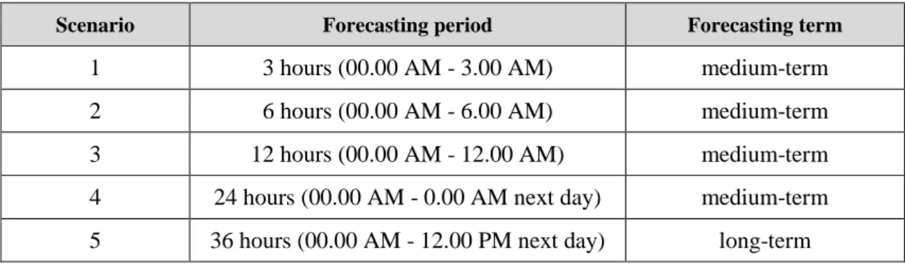
five different case studies (four case studies for medium-term forecasting and one case study for long-term

13

forecasting). The selected five case studies are detailed in Table 2.

14

As described in the previous section, there are 81 parameters in the T2FNN-PSO input data that are

15

obtained from the NWP and SCADA system. In this section, firstly, a T2FNN-PSO network should be

16

designed, and then this network is trained by input patterns including 81 parameters.

17

The design and training approach of the proposed T2FNN-PSO are explained in the following steps:

18

Step 1: The minimum and maximum variations of 81 input operating parameters are determined.

19

Step 2: For each of the 81 input parameters, three sets of Type-2 fuzzy are specified as “S”, “M” and

20

“L”. Here, Gaussian membership functions are selected for input parameters as shown in Fig. 8. It should

21

Table 2. The selected five different case studies for wind power forecasting

Scenario Forecasting period Forecasting term

1 3 hours (00.00 AM - 3.00 AM) medium-term

2 6 hours (00.00 AM - 6.00 AM) medium-term

3 12 hours (00.00 AM - 12.00 AM) medium-term 4 24 hours (00.00 AM - 0.00 AM next day) medium-term 5 36 hours (00.00 AM - 12.00 PM next day) long-term

17

Figure 8: Membership functions of the input parameters.

be noted that, the number of membership functions and UMF and LMF variances are specified using expert

1

knowledge.

2

Step 3: In this step, after designing the Type-2 fuzzifier, the neural network is designed. Here, a single

3

layer perceptron neural network is applied and trained by using the proposed PSO based training method.

4

Noteworthy that in case of utilizing a sole neural network, there is no option to consider uncertainties

5

associated with the input data. Moreover, the MLP neural network with several hidden layers should be

6

used because of the non-linear feature of the wind power forecasting problem. Needless to say, a single

7

layer MLP neural network is only capable of offering an acceptable performance for linear problems.

8

However, as one of the novelties of the paper, authors applied a Type-2 fuzzifier to the initial data before

9

entering to the neural network as input patterns. In fact, algorithm makes the initial input data fuzzy and

10

then the fuzzified data are applied to the neural network. This obligation provides several advantages for

11

the proposed method.

12

First, Type-2 fuzzifier performs as a mapping and therefore it converts the non-linear problem of the

13

wind power forecasting to a completely linear one. Therefore, it is possible to solve the linearized problem

14

using a MLP neural network without adding hidden layers. Second, it is capable of considering

15

uncertainties associated with the input data by employing Type-2 fuzzifier. Third, it greatly reduces the

16

computational cost by applying the proposed method to the given problem because of the high-speed and

17

efficient performance of single layer MLP neural networks without any hidden layers.

18

The proposed neural network has 486 neurons in its input layer; while number of output neurons is as

19

same as the number of scheduling hours for each case study. In the proposed structure, the outputs of Type-

20

2 fuzzifier are as inputs of the MLP neural network, and there are three Type-2 fuzzy membership

21

functions for each of parameters in the input patterns of the neural network. Considering the fact that Type-

22

18

2 fuzzifier has been utilized in this paper, there are two membership values (i.e. upper function and lower

1

function) corresponding to each of these three functions. Therefore, number of the fuzzified input values

2

corresponding to each parameter of input patterns will be 2×3=6.

3

As it has been mentioned, 81 parameters have been considered as the input variables of the neural

4

network. Accordingly, the number of neurons for the input layer of MLP neural networks can be calculated

5

as 81×6=486. Further details and mathematical expression of the number of neurons for the neural network

6

are provided in [31]. The time series of the wind farm are recorded from August 01 to August 31 for three

7

consecutive years from year 2013 to 2015 with one-hour interval [39, 40]. Therefore, the input data

8

includes 2232 patterns (i.e. for 24 hours × 31 days × 3 years). The forecasting data is given for up to 36

9

hours ahead at one-hour interval in cases of short-term and long-term forecasting. As mentioned, 75% of

10

the data set has been allocated to the learning procedure and the rest of patterns are used to evaluate the

11

performance of the fuzzy-neural network during the test procedure. Case studies related to 14-15th August,

12

2015 are shown in this paper to demonstrate the effectiveness of proposed method. Although it is possible

13

to consider the data recorded from one or several complete years as the input, the pattern related to a

14

specific month from several consecutive years has been employed to train fuzzy-neural network. This issue

15

prevents the problem of overtraining during training procedure of fuzzy-neural network due to a large

16

number of input data. However, because the diverse patterns of meteorological data in the location of wind-

17

farm during different seasons or even months, the trained network could not provide acceptable

18

performance with high accuracy.

19

A linear transfer function is used for the neurons in the output layer. The T2FNN-PSO training is

20

completed around 32s and the final root-mean-square error (RMSE) is completed about 0.015. It should be

21

noted that the simulation is performed on a personal computer with 2.93 GHz Pentium Dual-Core processor

22

and 2GB of random-access memory (RAM), running on MATLAB 7.10 software.

23

In order to evaluate the efficiency of trained T2FNN-PSO for the different case studies, it has been

24

verified by the testing sets of patterns. Performance of the proposed T2FNN-PSO is evaluated by values of

25

the mean absolute percentage error

(

MAPE) and the RMSE. These indexes can be computed as follows:

26

27

19

Table 3:The values of the MAPE and the RMSE for five case studies.

Number of case study Value of RMSE Value of MAPE

1 3.38 % 0.88 % 2 5.87 % 1.46 % 3 9.14 % 2.34 % 4 12.04 % 2.71 % 5 13.75 % 3.55 %

1

2 1 1

RMSE (actual Target(p) estimated Target(p))

N p

N _





 (6)

1

1 actual Target(p) estimated Target(p) MAPE 100 actual Target(p) N p N _   



₍₇₎

where N is the number of testing patterns. Table 3 shows the values of MAPE and RMSE (percentage of

2

full capacity) for five case studies. The obtained results confirm the accuracy of trained T2FNN-PSO for

3

five case studies. The scatter diagram for the wind power for five case studies is illustrated in Fig. 9. Each

4

point in this diagram is shown by (x, y) = (actual wind power, forecasted wind power). As it can be seen,

5

scattering level of the points in the proximity to “Exact fit line” illustrates T2FNN-PSO’s accuracy for

6

wind power estimation. Moreover, it can be observed that this accuracy has been maintained acceptable for

7

20

Figure 9: The scatter diagram for five case studies.

1

2

The cumulative distribution functions (CDF) of absolute percentage error (APE) for values of wind

3

power predictions are illustrated in Fig. 10.

4

21

Figure 10: CDF of APE curve for five case studies.

1

As can be seen in Fig. 10, about 99% of the total test patterns have APE of less than 5% in the case

2

study 1(i.e. 3h forecasting). Moreover, in the case study 2, about 97% of the total test patterns have APE of

3

less than 5%. This value for the other case studies is 90.6%, 88.2%, 81.5% of the total test patterns.

4

5

22

Figure 11: Comparison between the estimated and actual wind power for all case studies.

1

2

As shown in Fig. 10, it can be concluded that for all the case studies, small values of APEs (i.e. less than

3

5%) are more frequent (about 85%) than large APEs. The obtained results from simulations show that the

4

proposed T2FNN-PSO gives satisfactory estimation of wind power for all case studies. In order to evaluate

5

the sensitivity of algorithm to input parameters, the estimation of wind power for same scenarios has been

6

done when only the wind speed from the NWP model is used. In fact, nine other input variables of neural

7

network has been omitted. Results for considered scenarios are shown in Table 4.

8

Table 4:The values of the MAPE and the RMSE for five case studies NWP without auxiliary

parameters.

Number of case study Value of RMSE Value of MAPE

1 3.43 % 0.89 % 2 6.44 % 1.52 % 3 10.01 % 2.55 % 4 12.62 % 2.92 % 5 14.85 % 3.89 %

9

23

Obviously, the quality of obtained solutions are degraded without using auxiliary parameters. In this

1

regard, it should be mentioned that most of wind power prediction approaches use scaling curves to transfer

2

data obtained by NWP (i.e. measured at the height of 10 meters from ground) to the hub axis of wind

3

turbine. Utilizing these curves for wind speed, air pressure, humidity and other factures cause significant

4

error in estimating wind power. However, our approach compensate this deficiency by simultaneous using

5

of NWP data and SCADA system. Moreover, comparing to large number of previous researches in

6

literature which use only wind speed for power prediction, using several meteorological data can provide

7

more accurate predictions.

8

9

5.

C

ONCLUSION

10

In this paper, a novel intelligent method based on a hybrid T2FNN-PSO algorithm is presented for the

11

medium-term and long-term wind power forecasting under uncertain data. The proposed method can

12

effectively handle the uncertainties associated with the initial data obtained from the SCADA system, NWP

13

and measuring tools by using Type-2 fuzzy sets as Type-2 fuzzifier. The Type-2 fuzzifier layer transforms

14

noisy and uncertain input parameters to reliable linguistic variables. A new training method employing

15

PSO algorithm has been proposed for a fast and accurate offline training of the T2FNN-PSO.

16

The reliability and performance of the proposed approach have been verified by using the data of a real

17

wind farm. The simulation results show that the proposed T2FNN-PSO method can estimate the wind

18

power for all case studies with a reasonable accuracy. Moreover, the very simple structure of the proposed

19

method leads to reducing the computational time for training phase in online systems. Hence, this method

20

is a practical solution and can be applied for accurate wind power forecasting in power system control

21

centers.

22

24

References

1

[1] J. Jung, R.P. Broadwater, Current status and future advances for wind speed and power

2

forecasting, Renewable and Sustainable Energy Reviews, 31 (2014) 762–777.

3

[2] M. Jabbari, S. Hakimi, H. Afrakhte, A. Baghramian, A novel heuristic method for wind farm power

4

prediction: A case study, Electrical Power and Energy Systems, 63 (2014) 962–970.

5

[3] Pinson P, Christensen LEA, Madsen H, Sørensen P, Donovan MH, Jensen LE. Regime-switching

6

modelling of the fluctuations of offshore wind generation. J Wind Eng Ind Aerodyn 2008;

7

96(12):2327–47.

8

[4] Kariniotakis G, Nogaret E, Stavrakakis G. Advanced short-term forecasting of wind power

9

production. In: European wind energy conference EWEC’97, Ireland; 1997.

10

[5] Damousis IG, Dokopoulos P. A fuzzy model expert system for the forecasting of wind speed and

11

power generation in wind farms. In: 22nd IEEE international conference on power industry

12

computer applications (PICA), Sydney, NSW; 2001.

13

[6] Ramírez-Rosado IJ, Fernández-Jiménez LA. Next-day wind farm electric energy generation

14

forecasting using fuzzy time-series. In: International conference on modeling, identification, and

15

control, Innsbruck, Austria; 2003.

16

[7] Kariniotakis G, Nogaret E, Dutton AG, Halliday JA, Androutsos A. Evaluation of advanced wind

17

power and load forecasting methods for the optimal management of isolated power systems. In:

18

European wind energy conference EWEC’99, Nice, France; 1999.

19

[8] Bossanyi EA. Short-term wind prediction using Kalman filters. Wind Eng 1985; 9(1):1–8.

20

[9] Alpay S, Bilir L, Ozdemirny S, Ozerdem B. Wind speed time series characterization by Hilbert

21

transform. Int J Energy Res 2006;30(5):359–64.

22

[10] Abdel-Aal RE, Elhadidy MA, Shaahid SM. Modeling and forecasting the mean hourly wind speed

23

time series using GMDH-based abductive networks. Renew Energy 2009; 34(7):1686–99.

24

[11] Potter CW, Negnevistky M. Very short-term wind forecasting for Tasmanian power generation.

25

IEEE Trans Power Syst 2006;21(2):965–72.

26

[12] El-Fouly THM, El-Saadany EF, Salama MMA. Grey predictor for wind energy conversion systems

27

output power prediction. IEEE Trans Power Syst 2006; 21(3):1450–2.

28

[13] Negnevitsky M, Johnson P, Santoso S. Short term wind power forecasting using hybrid intelligent

29

systems. In: IEEE power engineering society general meeting, Tampa, FL; 2007.

30

[14] Sanchez Ismael. Short-term prediction of wind energy production. Int J Forecast 2006;

31

25

[15] Fan Shu, Liao JR, Yokoyama R, Chen Luonan, Lee Wei-Jen. Forecasting the wind generation using

1

a two-stage hybrid network based on meteorological information. IEEE Trans Energy Convers

2

2009;24(2):474–82.

3

[16] Jursa R. Wind power prediction with different artificial intelligence models. In: European wind

4

energy conference EWEC’07, Milan, Italy; 2007.

5

[17] Barbounis TG, Theocharis JB, Alexiadis MC, Dokopoulos PS. Long-term wind speed and power

6

forecasting using local recurrent neural network models. IEEE Trans Energy Convers

7

2006;21(1):273–84.

8

[18] Mario JD, Cros D, Riquelme J. Short-term wind power forecast based on ARX models. J Energy

9

Eng 2007; 133(3):172–80.

10

[19] Yamaguchi A, Ishihara T, Sakai K, Ogawa T, Fujino Y. A physical–statistical approach for the

11

regional wind power forecasting. In: European wind energy conference EWEC’07, Milan, Italy; 2007.

12

[20] Fugon Lionel, Juban Jérémie, Kariniotakis G. Data mining for wind power forecasting. In:

13

European wind energy conference EWEC’08, Brussels, Belgium; 2008.

14

[21] Kusiak A, Zheng H-Y, Song Z. Wind farm power prediction: a data-mining approach. Wind Energy

15

2009; 12(3):275–93.

16

[22] Marti I, Kariniotakis G, Pinson P, Sanchez I, Nielsen TS, Madsen H., et al. Evaluation of advanced

17

wind power forecasting models – results of the Anemos Project. In: Proceedings of the 2006

18

european wind energy conference and exhibition; 2006.

19

[23] Bouzgou H, Benoudjit N. Multiple architecture system for wind speed prediction. Appl Energy

20

2011;88:2463–71.

21

[24] Qian Z, Kin Keung L, Dongxiao N, Qiang W. Wind park power forecasting models and

22

comparison. In: Proceedings of the 2012 fifth international joint conference on computational

23

sciences and optimization (CSO); 2012. p. 27–31.

24

[25] Xiao Q, Cong J, Jun W. Online clustering for wind speed forecasting based on combination of RBF

25

neural network and persistence method. In: Proceedings of the 2011 chinese control and decision

26

conference (CCDC); 2011. p. 2798–802.

27

[26] Shi J, Guo J, Zheng S. Evaluation of hybrid forecasting approaches for wind speed and power

28

generation time series. Renew Sustain Energy Rev 2012; 16:3471–80.

29

[27] Liu H, Tian H-q, Li Y-f. Comparison of two new ARIMA–ANN and ARIMA–Kalman hybrid

30

methods for wind speed prediction. Appl Energy 2012; 98:415–24.

31

[28] Li G, Shi J, Zhou J. Bayesian adaptive combination of short-term wind speed forecasts from

32

neural network models. Renew Energy 2011; 36:352–9.

33

26

[29] Haque AU, Mandal P, Kaye ME, Meng J, Chang L, Senjyu T. A new strategy for predicting short-

1

term wind speed using soft computing models. Renew Sustain Energy Rev 2012; 16:4563–73.

2

[30] Guo Z, Zhao J, Zhang W, Wang J. A corrected hybrid approach for wind speed prediction in Hexi

3

Corridor of China. Energy 2011; 36:1668–79.

4

[31] Sharifian A, Sharifian S. A new power system transient stability assessment method based on

5

Type-2 fuzzy neural network estimation. Int J Electr Power Energy Syst 2015; 64:71–87.

6

[32] Charabi Y.Arabian summer monsoon variability: teleconexion to ENSO and IOD. Atmospheric

7

Research 2009; 105–117.

8

[33] Kariniotakis GN, Pinson P. Uncertainty of short-term wind power forecasts a methodology for

9

on-line assessment. In: International Conference on Probabilistic Methods Applied to Power Systems,

10

Ames, IA 2004.

11

[34] Mohammadzadeh A, Ghaemi S. Synchronization of chaotic systems and identification of

12

nonlinear systems by using recurrent hierarchical type-2 fuzzy neural networks. ISA Transactions

13

2015; 58:318–329.

14

[35] Lou C.W, Dong M.C. A novel random fuzzy neural networks for tackling uncertainties of electric

15

load forecasting Original Research Article. Int. J Electr. Power Energy Syst. 2015; 73:34-44.

16

[36] Kennedy J,Eberhart R. Particle swarm optimization. IEEE Conf Neural network 1995; 4:1942-8.

17

[37] Kayacan E, Khanesar M.A. Chapter 8 – Hybrid Training Method for Type-2 Fuzzy Neural

18

Networks Using Particle Swarm Optimization. Fuzzy Neural Networks for Real Time Control

19

Applications 2016; 133–160.

20

[38] Vestas company site [On-line]. http://www.vestas.com/

21

[39] National Climate Data and Information Archive, [On-line]. Available:

22

http://www.climate.weatheroffice.gc.ca/

23

[40]Real time wind & weather report [On-line]. Available: https://www.windfinder.com/

24

[41] Web Mapping Service developed by Google [On-line]. https://maps.google.com/

25

[42] Weather Spark [On-line]. https://weatherspark.com/

26