N
EURAL
N
ETWORK
B
ASED
I
MAGE
R
EPRESENTATION FOR
S
MALL
S
CALE
O
BJECT
R
ECOGNITION
A thesis submitted in fulfilment of the requirements for the degree of Doctor of Philosophy
HIEU MINH BUI
M.Eng. in Electronic and Computer Engineering – RMIT University, Vietnam B.Eng. in Electronic and Communication Engineering – Danang University of Technology,
Vietnam
School of Engineering
College of Science, Engineering and Health RMIT University
ii
D
ECLARATION
I certify that except where due acknowledgement has been made, the work is that of the author alone; the work has not been submitted previously, in whole or in part, to qualify for any other academic award; the content of the thesis is the result of work which has been carried out since the official commencement date of the approved research program; any editorial work, paid or unpaid, carried out by a third party is acknowledged; and, ethics procedures and guidelines have been followed.
Hieu Minh Bui November 14th, 2018
iii
A
CKNOWLEDGEMENTS
To mark the completion of my PhD thesis, I would like to express my appreciation to many people and organizations who had contributed to transform my life from a crowd follower into an independent thinker.
The first word I want to reserve for the AusAid program of the Australian government. Their scholarship for me to study master program in RMIT university has been a turning point in my life. In fact, it was the foundation that launched me up to the PhD candidature.
Next, I would like to specially thank my supervisors Prof Margaret Lech, Dr Eva Cheng, Dr Katrina Neville, Dr Richardt Wilkinson, and Prof Ian Burnett, who have given me continuous support to all problems related to my PhD. Their help has made the challenging PhD candidature become feasible and much less stressful.
Finally, I want to thank my parents, who gave me all the physical power, mental power, and the necessary freedom to make choices for my life and push them forward.
iv
L
IST OF
P
UBLICATIONS
Journal papers
:
[1] H. M. Bui, M. Lech, E. Cheng, K. Neville, and I. S. Burnett, "Object Recognition Using Deep Convolutional Features Transformed by a Recursive Network Structure," IEEE Access, vol. 4, pp. 10059-10066, 2016.
Conference papers
:
[1] H. M. Bui, M. Lech, E. Cheng, K. Neville, and I. S. Burnett, "Using gray-scale images for object recognition with convolutional-recursive neural network," in 2016 IEEE Sixth International Conference on Communications and Electronics (ICCE), 2016, pp. 321-325. [2] H. M. Bui, M. Lech, E. Cheng, K. Neville, R. Wilkinson, and I. S. Burnett, "Randomized dimensionality reduction of deep network features for image object recognition," in Recent Advances in Signal Processing, Telecommunications & Computing (SigTelCom), 2018 2nd International Conference on, 2018, pp. 136-141.
v
T
ABLE OF
C
ONTENTS
Declaration... ii Acknowledgements ... iii List of Publications ... iv Table of Contents ... vList of Figures ... viii
List of Tables ... x
Abstract ... 1
Introduction ... 3
1.1 Preview ... 3
1.2 Background and Problem Statement ... 3
1.3 Thesis Aim ... 6
1.4 Thesis Research Questions ... 6
1.5 Thesis Scope ... 6
1.6 Thesis Contributions ... 7
1.7 Thesis Structure ... 8
Literature review ... 9
2.1 Preview ... 9
2.2 Object Recognition Pipeline ... 9
2.3 Feature extraction – the road to machine learning ... 12
2.3.1 Preprocessing and generic enhancement ... 12
2.3.2 Evolution of object recognition features ... 15
2.3.3 Machine learning ... 17
vi
2.5 Classifiers ... 36
2.6 Benchmark datasets ... 38
2.7 Summary ... 40
Impact of colour in object recognition ... 42
3.1 Preview ... 42
3.2 Effect of Disregarding Colours ... 42
3.2.1 The evolution of image features ... 43
3.2.2 Image object classification framework ... 44
3.2.3 Gray-scale feature extraction ... 45
3.2.4 Classification ... 48
3.3 Summary ... 54
Neural networks and transfer learning ... 55
4.1 Preview ... 55
4.2 Neural Networks ... 55
4.2.1 Going deep to find a good representation ... 56
4.2.2 Transfer learning ... 58
4.2.3 The AlexNet-RNN feature extractor ... 60
4.2.4 Classification ... 62
4.3 Summary ... 70
Dimensionality reduction and feature encoding ... 71
5.1 Preview ... 71
5.2 Dimensionality reduction for DNN features ... 71
5.2.1 Dimensionality Reduction With Random Orthogonal Projection ... 71
5.2.2 Dimensionality reduction by mimicking t-SNE ... 85
5.3 Fisher Vector using Infinite Gaussian Mixture ... 89
5.3.1 Image coding and the generative model... 89
vii
5.3.3 Object recognition using Fisher vector ... 99
5.3.4 Extend the dictionary size ... 101
5.4 Summary ... 106
Conclusions and future work ... 108
6.1 Preview ... 108
6.2 Findings Regarding the Research Questions ... 108
6.3 Research Summary and Conclusion ... 109
6.4 Future Research Directions ... 110
viii
L
IST OF
F
IGURES
Figure 1.1 - A typical recognition system [3]. ... 4
Figure 2.1 - Representation of a digital image. ... 10
Figure 2.2 - A toy example for classification; not linearly separable (left); and linearly separable (right). ... 11
Figure 2.3 - Effects of popular enhancing techniques on data (visualized using random data generated by two Gaussians). ... 14
Figure 2.4 - Locality of texture in an image (sample from ImageNet [28]). ... 15
Figure 2.5 - Example of expected clusters of object images (samples from ImageNet [28]). 17 Figure 2.6 - Visualization of a Gaussian distribution in 2-dimensional space. ... 19
Figure 2.7 - Visualization of 3 Gaussian clusters (with different mean vectors and covariance matrices) in 2-dimensional space. ... 19
Figure 2.8 - Conceptual idea of an autoencoder. ... 22
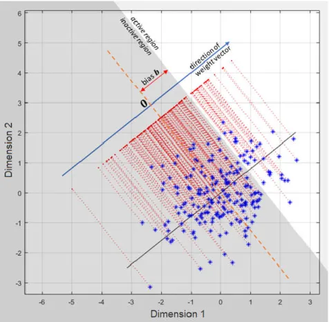
Figure 2.9 – Visualizing the operation of a neuron in 2D space. ... 27
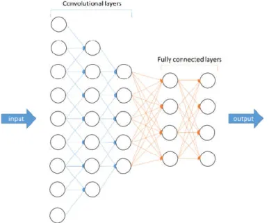
Figure 2.10 - A typical structure of a deep neural network for object recognition purpose. .. 28
Figure 2.11 - Structure of ZF Net (top) and visualization of features learned by neurons in its layers in accordance with the input (bottom), reproduced from [95]. ... 30
Figure 3.1 - COIL20 object library. ... 43
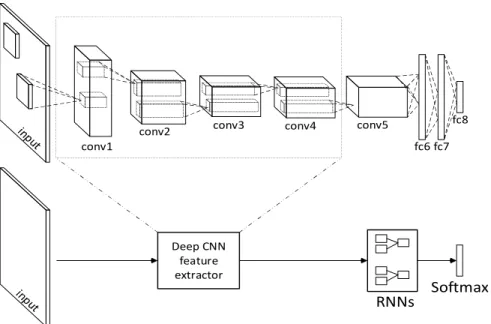
Figure 3.2 - Convolutional-Recursive object recognition system. ... 46
Figure 3.3 - Structure of Convolutional NN (left) and Recursive NN (right). ... 47
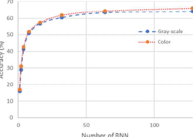
Figure 3.4 - Performance of RGB and gray-scale images versus number of RNNs used. ... 49
Figure 3.5 - Objects in the W-RGBD data set. ... 50
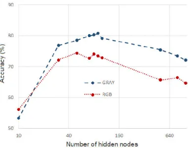
Figure 3.6 - Performance of RGB and gray-scale images versus number of hidden nodes used. ... 52
Figure 3.7 – Object recognition accuracy of RGB and gray-scale images in Caltech101 dataset versus number of RNNs used. ... 53
Figure 3.8 – Sample images in Caltech101 dataset with cluttered background ... 54
Figure 4.1 - Structures of AlexNet (top) and the structure of the proposed system with AlexNet applied as feature extractor (bottom). ... 59
Figure 4.2 - Structure of the CNN layer (top) and the RNN layer (bottom). ... 60
ix Figure 4.4 - Recognition accuracy for features extracted from several selected layers of
AlexNet-2014. ... 65
Figure 4.5 - Example images from ImageNet and W-RGBD dataset. ... 69
Figure 5.1 - Histogram of pairwise cosine distance between filters in each layer of the pre-trained AlexNet. ... 75
Figure 5.2 – Evolution of histogram of pairwise cosine distance between filters in each layer of AlexNet during training. ... 76
Figure 5.3 - Structure of QR-based recognition pipeline with pre-trained AlexNet employed as feature extractor. ... 78
Figure 5.4 – Low-dimensional embedding using neural network guided by t-SNE. ... 87
Figure 5.5 – 2D t-SNE visualization of 3 image features selected randomly from CNN net output (left) and the result of mimic mapping using a 34-node neural network (right)... 87
Figure 5.6 – Example of indistinguishable objects in the Washington-RGBD dataset. ... 89
Figure 5.7 - Example of expressing images using sparse terms (images form ImageNet2012). ... 91
Figure 5.8 - Cluster size of SIFT features when fitting a GMM using the EM algorithm. ... 92
Figure 5.9 - Cluster size of cv-5 features when fitting a GMM using the EM algorithm. ... 92
Figure 5.10 - Cluster size of fc6 features when fitting a GMM using the EM algorithm. ... 93
Figure 5.11 - Illustration of data encoding using hard-assigned Mixture Model residuals. ... 94
Figure 5.12 – Illustration of encoding data using sparse coding residuals. ... 98
Figure 5.13 – Histogram of pair-wise cosine distance between bases learnt by sparse coding. ... 102
Figure 5.14 - Modeling error versus dictionary size (left) and corresponding sparsity level (right) using Matching Pursuit on different k-means approaches... 105
x
L
IST OF
T
ABLES
Table 2.1 - Popular preprocessing techniques. ... 14
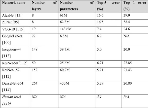
Table 2.2 - Summary of well-known deep neural networks in ImageNet recognition (10-crop, single-model evaluation). ... 33
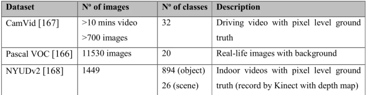
Table 2.3 – Notable datasets available for research in visual object recognition and semantic image segmentation. ... 38
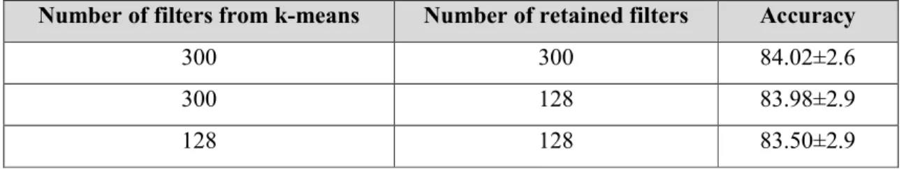
Table 3.1 - Comparison to other methods (Accuracy = mean ± standard deviation). ... 51
Table 3.2 - Improved accuracy with feature selection on gray-scale images. ... 51
Table 4.1 - Effect of using RNN on recognition accuracy (applied on activations of layer 4 of AlexNet-2014. ... 64
Table 4.2 - Performance difference between of features from AlexNet-2014 and AlexNet-2012 across layers. ... 65
Table 4.3 - Performance comparison of the proposed method with previous works. ... 67
Table 4.4 - Object classification accuracy using AlexNet-2014 with 128 RNNs and activation from layer 4. ... 69
Table 5.1 - Layer structure of the AlexNet [98]. ... 73
Table 5.2 - Classification result on Caltech101 dataset using pre-trained AlexNet as feature extractor. ... 81
Table 5.3 - Classification result on Caltech256 dataset using pre-trained AlexNet as feature extractor. ... 82
Table 5.4 - Classification result on Caltech 101 with original images’ aspect ratio. ... 83
Table 5.5 - Classification result on Caltech 256 with original images’ aspect ratio. ... 83
Table 5.6 - Recognition accuracy of state-of-the-art approaches on Caltech101 dataset. ... 85
Table 5.7 - Recognition accuracy of state-of-the-art approaches on Caltech256 dataset. ... 85
Table 5.8 - Classification results on the W-RGBD dataset using mimicking low-dimensional embedding. ... 88
Table 5.9 - Classification results on the Pascal 2007 dataset in comparison with other approaches. ... 100
Table 5.10 - Classification results on the Caltech-101 dataset in comparison with other approaches. ... 101
Table 5.11 - Comparison of modeling accuracy between sparse coding (SC) and matching pursuit (MP) using the same set of 200 sparse bases. ... 102
xi
List of Abbreviations
Abbreviation Description 2D/3D 2/3 Dimension
ANOVA Analysis of variance
BoF Bag of Features
BoW Bag of Word
CLIQUE Clustering in Quest
CNN Convolutional Neural Network
CPU Central Processing Unit
cv-i ith convolutional layer (in deep network)
DBN Deep Belief Nets
DBSCAN Density-based spatial clustering of applications with noise
DNN Deep Neural Network
EM Expectation–Maximization
EMK Efficient Match Kernel
fc-i ith fully-connected layer (in deep network)
FIM Fisher Information Matrix
FNN Feedforward Neural Network
FNN Fully-connected Neural Network
FV Fisher Vector
GAN Generative Adversarial Networks
GB Gigabyte
GMM Gaussian Mixture Model
GPU Graphical Processing Unit
HPM Hierarchical Matching Pursuit
ICA Independent Component Analysis
LASSO Least Absolute Shrinkage & Selection Operator
L-BFGS Low memory Broyden–Fletcher–Goldfarb–Shanno optimization
LRN Local Response Normalization
MHz Mega-hertz
xii
Abbreviation Description
MLP Multi-Layer Perceptron
NVIDIA a company specializing in graphical computing hardware (http://www.nvidia.com)
ORB Oriented FAST and Rotated BRIEF
PCA Principal Component Analysis
RAM Random-access memory
RBM Restricted Boltzmann Machine
RCNN Recursive Convolutional Neural Network
R-CNN Region-based Convolutional Neural Network
ReLU Rectifier Learning Unit
RGB Red Green Blue
SC Sparse Coding
SCFV Sparse Coding Fisher Vector
SCG Scaled Conjugate Gradient
SGD Stochastic Gradient Descent
SIFT Scale-Invariant Feature Transform
SP Spatial Pooling
SPM Statistical Parametric Mapping
SPP Spatial Pyramid Pooling
SRP Sparse Random Projection
SURF Speeded Up Robust Features
SVM Support Vector Machines
t-SNE t-distributed Stochastic Neighbour Embedding
VLAD Vector of Locally Aggregated Descriptors
1
A
BSTRACT
Object recognition can be abstractedly viewed as a two-stage process. The features learning stage selects key information that can represent the input image in a compact, robust, and discriminative manner in some feature space. Then the classification stage learns the rules to differentiate object classes based on the representations of their images in feature space. Consequently, if the first stage can produce a highly separable features set, simple and cost-effective classifiers can be used to make the recognition system more applicable in practice. Features, or representations, used to be engineered manually with different assumptions about the data population to limit the complexity in a manageable range. As more practical problems are tackled, those assumptions are no longer valid, and so are the representations built on them. More parameters and test cases have to be considered in those new challenges, that causes manual engineering to become too complicated. Machine learning approaches ease those difficulties by allowing computer to learn to identify the appropriate representation automatically. As the number of parameters increases with the divergence of data, it is always beneficial to eliminate irrelevant information from input data to reduce the complexity of learning. Chapter 3 of the thesis reports the study case where removal of colour leads to an improvement in recognition accuracy.
Deep learning appears to be a very strong representation learner with new achievements coming in monthly basic. While training the phase of deep structures requires huge amount of data, tremendous calculation, and careful calibration, the inferencing phase is affordable and straightforward. Utilizing knowledge in trained deep networks is therefore promising for efficient feature extraction in smaller systems. Many approaches have been proposed under the name of “transfer learning”, aimed to take advantage of that “deep knowledge”. However, the results achieved so far could be classified as a learning room for improvement. Chapter 4 presents a new method to utilize a trained deep convolutional structure as a feature extractor and achieved state-of-the-art accuracy on the Washington RGBD dataset.
Despite some good results, the potential of transfer learning is just barely exploited. On one hand, a dimensionality reduction can be used to make the deep neural network representation even more computationally efficient and allow a wider range of use cases. Inspired by the structure of the network itself, a new random orthogonal projection method for the dimensionality reduction is presented in the first half of Chapter 5. The t-SNE mimicking
2 neural network for low-dimensional embedding is also discussed in this part with promising results.
In another approach, feature encoding can be used to improve deep neural network features for classification applications. Thanks to the spatially organized structure, deep neural network features can be considered as local image descriptors, and thus the traditional feature encoding approaches such as the Fisher vector can be applied to improve those features. This method combines the advantages of both discriminative learning and generative learning to boost the features performance in difficult scenarios such as when data is noisy or incomplete. The problem of high dimensionality in deep neural network features is alleviated with the use of the Fisher vector based on sparse coding, where infinite number of Gaussian mixtures was used to model the feature space. In the second half of Chapter 5, the regularized Fisher encoding was shown to be effective in improving classification results on difficult classes. Also, the low-cost incremental k-means learning was shown to be a potential dictionary learning approach that can be used to replace the slow and computationally expensive sparse coding method.
3
I
NTRODUCTION
1.1
P
REVIEW
Object recognition is one of the key areas in computer vision, which aims to help computer to see the world in a way similar to the capability of a human. Consequentially, the design of a computer object recognition system bears much resemblance to the biological structure of the visual system. In a human, the snapshot of the world starts at the reception layer of the human visual system in the retina, which consists of millions of photoreceptor cells, each converting light intensity into neural signals to be sent to higher layers [1]. Correspondingly, the first visual reception layer for a computer is the image sensor, which comprises millions of pixels performing a similar function to the photoreceptor cells on the retina. In both regimes, a moment of the world is represented by a set of a very lager number of points arranged in a spatial order, each containing information about the light intensity exposed at the respective small local region.
At the end of the visual system, in almost any circumstance, a human can simultaneously extract a lot of useful information about the world being seen, including which objects are present. The target for computer vision is to build a similar function on a computer to make it do object recognition. Unfortunately, human knowledge about the brain is also very limited. Therefore, for computer vision, the scope of useful information has to be limited for each target application. On one hand this is to reduce the computational complexity, and on the other hand, to keep a clear and tractable application design. Nevertheless, in both scenarios, the vision system needs to extract the key image descriptors,e.g. an object label, a colour profile, a posture, etc. This amount of information is extremely small compared to the set of pixels at the starting point. Intuitively, in the process of recognition, the task of either human visual system or the computer involves reducing the amount of information. Reduction always involves loss, so the question is how to make the loss selective, while presenting the remaining data in a consistently useful way.
1.2
B
ACKGROUND AND
P
ROBLEM
S
TATEMENT
Visual object recognition has been around for more than 50 years, been through many turn overs [2]. The diversity of recognition methods is large, but in the coarse view, they all follow
4 a similar pipeline structure as shown in Figure 1.1. The feature learning phase identifies the representative information (features) from input images to form a new representation which best separates the object classes. This stage could be subdivided into a feature extraction step, that identifies important image information, and an optional feature encoding step, that transforms the identified information in a more efficient way. The classification phase hypothesizes the object models in the feature space and defines the hyper plains to separate them. Together, if the feature learning phase can form a good representation for the image which highlighted the discriminative features, then the task for the classification phase will be easy. In turn, the overall efficiency is largely dependent on the efficiency of the first stage.
Figure 1.1 - A typical recognition system [3].
There has been a large number of different approaches to extract key information from image targeting object recognition, ranging from manual design to automatic learning. However, the performance of deep learning approaches, which started in 2011 had surpassed all previous methods and continuously set new records in different classification tasks. In particular, deep neural networks have been shown to be able to pick up the most relevant details that benefit the target application, while maintaining a great extent of invariance and robustness thanks to the power of back propagation that passes down the system error to every processing stage and allows for the finest adjustments. Deep neural networks excel in large scale visual tasks. In addition, it has also shown to have a great generalization capability to transfer from one domain to the other. The power of deep learning is reinforced daily with the development of new dedicated high-performance hardware. However, on the down side, that dedicated hardware is an obstacle that restricts the use of deep learning in many applications. More than that, a deep neural network requires a very large amount of training data, that may be not available in many cases. In turn, a new trend is to utilize pre-trained deep models to improve recognition in smaller application spaces. Fine tuning the network parameters with small adjustment steps is a popular choice to adapt the network to a new distribution. However, such approaches have not shown much improvement due to the limitation of training data.
5 There are mainly two regimes of methods for classification problems, discriminative approaches and generative approaches. Discriminative approaches try to model the conditional probability ( | ) of the output provided the input, while the generative approaches model the joint probability ( , ) of the input and the output. In simple terms, if the task is to differentiate a car and a motorbike, then the discriminative approach tries to find the details that exist on one type of the object but not on the other, e.g. a car has 4 wheels, but a bike only has two. Our capability to imagine the occluded part of an object in an image is an example of generative learning, where we use the pre-learned model of the object to supplement information about the missing pieces. Contrarily, generative approaches try to model what the car looks like and what the motorbike looks like. Consequently, discriminative approaches need to process a smaller amount of information and can make more aggressive assumptions on the data. This possibly explains the preference of the research community toward discriminative approaches, and to explain why they are more efficient. However, generative approaches hold the potential to deal better with incomplete data, where some details are not available for discriminative approaches to work. In fact, all images of objects are incomplete in general due to the loss occurring when projecting a 3D object onto a 2D plane of the camera sensor. Therefore, a sustainable image representation is expected to take advantage of both of those regimes.
In small-scale settings, apart from the recognition accuracy, the computational cost and memory footprint may be more relevant. These concerns can be addressed by reducing irrelevant information from the image representation. There are many techniques available for dimensionality reduction, but they were designed for general purpose data, and may not be the optimal choice for deep image features. As deep neural networks for large scale object recognition all have similar structure in general, it is expected that image features extracted by these networks have some generic properties that one can exploit to simplify the post extraction processing, including dimensionality reduction. In addition, by using deep neural network features, one is ready with a clean and compact set of image information for the discrimination purpose. The remaining task is how to handle these features in a cost-effective way while preserving and possibly enhancing the classification result on the target domain. As a result, this thesis will investigate the use of deep neural network features in different settings and explores the potential of improving these features using traditional techniques with the aid of human knowledge.
6
1.3
THESIS AIM
The thesis aim is to optimize an image object recognition system based on the deep neural network features to achieve high classification accuracy, and low computational and data requirements. In order to achieve these goals, the thesis investigates two types of object recognition methods. The first method is where the objective is to achieve a low computational cost, and the second method is where, the objective is to achieve a high classification accuracy. To achieve a low computational cost, research is conducted to find an appropriate transformation that will map deep neural network features to a lower dimensional space using low computational cost transformation techniques. To achieve a high recognition accuracy, this study investigates subspaces and new representations that allow for the efficient separation of the object classes while keeping the cost within prescribed limits.
1.4
T
HESIS
R
ESEARCH
Q
UESTIONS
1. Does retaining more information from an object image improve the recognition accuracy? How to determine which information is relevant?
2. How to learn a large dictionary of objects represented by high dimensionality data? Is there an alternative that surpasses the k-means technique in both processing speed and discriminative power?
3. Which properties of deep neural networks can be exploited to improve the efficiency of object recognition based on the network activation features?
4. How can the power of the discriminative learning and the generative learning approaches be combined to improve the quality of the object recognition features?
1.5
T
HESIS
S
COPE
This research focuses on improving the feature extraction stage of the object recognition systems. While multiple means can be used to present an image object, the topics discussed in this research are only concerned with the recognition of object labels in 2D static images. Multi-modal recognition such as 3D representations, depth masks and thermal maps are not considered.
7 This thesis investigates image object recognition methods in cases where both, the amount of training images and the computational resources are limited. The research presented in this thesis is not aimed as designing a universal state-of-the art recognition algorithm applicable to an arbitrary input domain. Instead, the focus is to utilize recent advancements in the large-scale recognition technology to improve the recognition performance in an application involving relatively small numbers (no more than a few hundreds) of classes. Such applications are typical in many fabrication, sorting, storage and retail processes.
There is a large research overlap between object localization (determining the location of a given object in an image) and object recognition (assigning a label to the object depicted by an image) tasks. The research presented in this thesis is only concerned with the object recognition task.
1.6
THESIS CONTRIBUTIONS
This thesis describes a number of original methods and experiments designed and conducted by the author. The main contributions of the thesis can be summarized as follows:
Providing a comprehensive and self-contained literature review of computer visual object recognition research. The review is focused on very recent deep learning techniques and the transfer approaches to apply deep learning in small scale applications.
Investigating the differences between image object recognition based on gray-scale images and object recognition based on colour images. Proposing a number of useful practical enhancements to improve the recognition accuracy, while keeping the computational cost low when using gray-scale images as input to the object recognition pipeline.
Proposing a new low computational- and low data-cost image object recognition approach, that utilizes a pre-trained deep neural network to generate activation features and a random recursive network to optimize these features before using them to train the classifier for object recognition.
Proposing a new computationally efficient feature dimensionality reduction method using randomization inspired by the deep neural network properties.
Proposing a new high-accuracy hybrid discriminative-generative feature encoding method to enhance deep neural network features.
Proposing a new low-cost dictionary learning for high dimensional data with the potential to be used for encoding deep neural network features.
8
1.7
THESIS STRUCTURE
This thesis consists of six chapters, which discuss the research context of the visual object recognition field and the experiments conducted by the author in order to provide answers to the abovementioned research questions. The thesis is organized as follows:
Chapter 1 describes the research background and the research problem. This is followed by the thesis aims, research questions, thesis scope, thesis contributions and the thesis structure.
Chapter 2 provides an overview of the visual object recognition literature. It discusses the advantages and limitations of the existing techniques and identifies research gaps addressed in the thesis.
Chapter 3 describes an experiment where the author compares the object recognition based on gray-scale images against the object recognition based on colour images. The results show that in specific settings, the application of the gray-scale images significantly improves the recognition accuracy compared to the approach with colour images, with a lower computational cost.
Chapter 4 describes a low computational cost approach using a recursive random network to optimize the deep neural network features. The experimental results show that this relatively simple and low-cost approach produces very good image object representations and achieves state-of-the-art recognition accuracy performance on the Washington RGBD dataset.
Chapter 5 describes two further approaches proposed by the author with the aim to achieve either low computational cost, or better recognition accuracy. Both methods are applied on the deep neural network features. To achieve low computational cost, a simple yet effective feature dimensionality reduction method is proposed. This approach uses randomization inspired by the deep neural network properties, and as such it is shown to work better than other randomized alternatives at a similar computational cost. To achieve better recognition accuracy, a hybrid discriminative-generative feature encoding method is proposed to enhance the deep neural network features. The test results show that this method achieves good overall accuracy while being more robust to noise compared to other methods.
Chapter 6 concludes the thesis. Thesis findings are summarized in the context of the initial research questions. Thesis limitations and potential future research directions are also outlined.
9
L
ITERATURE REVIEW
2.1
P
REVIEW
This chapter provides an overview of the visual object recognition literature, discusses the advantages and limitations of the existing techniques, and identifies research gaps addressed by this thesis.
Visual understanding is the key factor for a human to interact with the surrounding world. A big part of that understanding is the capability to identify objects. In turn, there is a great interest to equip computers with a similar ability. Knowledge in mathematics and neuroscience is utilized the most in converting images from pixel space to feature space that better reveals the identification of objects. Along that journey so far, various approaches had been proposed, and various test cases were also built to test those inventions. It turns out that the most successful model to date is the one that mostly resemblesthe structure of the human brain itself.
2.2
O
BJECT
R
ECOGNITION
P
IPELINE
Animals are gifted with the ability to sense the world through the visual system, which provides the most complete description about the physical matter of their surroundings at every moment. Humans, in turn have utilized that gift to the largest extent that contributed to development of civilization. Visual cognition consists of multiple parts, and recognition is one of the most important branches. The ability to identify different objects is a fundamental need for humans to interact with the world. With advancement of technology, it is expected that machines can be used to replace humans in many scenarios. As a result, it is necessary to equip machines with the capability to identify different objects using visual means or expressing in technical term the capability to do visual object recognition.
The visual system in humans contains several parts. Information starts being collected at the densely distributed photoreceptor cells in the retina of the eyes, passing through multiple parts of the visual cortex in the brain with hundreds of millions of neural cells connected [4] and being converted into cognitive information that describes the scene in sight [5]. It is not clearly understood by neuroscientists how the brain works, but it is clear that our brain has ability to extract the critical details that explain the objects in order to identify them [6]. For example, to
10 differentiate a dog and a table, we immediately know that the dog may be furry, but the table is not. We can convert a furry representation acquired by our eyes into the semantic representation of the animal, and we can also do the reversed process by imagining the appearance of a dog when being fed by just the word “dog”. We want to train the machine for similar capabilities. We want them to be able to pick out the key information from some input. We want them to learn rules on those key details to decide whether a certain kind of object is present. Sometimes, we also want the computer to model the appearance of the object such that it can visualize the object provided by some high-level semantic stimuli. In formal terms, we identify key information through a feature extraction process, we learn decision rules by training classifiers, and we hypothesize the objects by learning generative models.
Visual object recognition on computers deals with images. On digital cameras, images are captured by a sensor with millions of pixels, which is a resemblance of the retinal photoreceptors in our eyes. In the past, with black-white images, each pixel was expressed as a single number. However, today cameras with colours required at least 3 numbers per pixel, such as the example shown in Figure 2.1. Sometimes, with extra modality such as depth, thermality, more numbers are needed to depict the image value at each location. This results in a very large representation for each snapshot, which makes it very difficult to learn the rule to separate different images. The first step in doing recognition on computers is thus to compress the information for tractable processing.
Figure 2.1 - Representation of a digital image.
In reality, objects are rarely placed in an isolated scene. In other words, an image of an object usually contains other objects and a background. In digital representation, every pixel in an image is just a set of numbers, therefore there is no known way to teach a computer to focus just on the object and ignore the other elements. That application specific “attention” will be another target for the computer to learn in doing object recognition. It means that the
11 recognition system has to learn to select the important information of the image and remove the irrelevant information with respect to the aimed object recognition task. In short, that information must be representative of one kind of object but not to all other kinds.
In addition, most objects in general are 3-dimensional (3D) structures. In contrast, most images captured by digital cameras are 2-dimensional representations. The process to convert from a 3D space data point into a 2D image is always lossy, and thus every image is an incomplete representation of the object. Depend on the capturing condition such as lightning, viewing angle, motion speed, camera’s specifications, images of the same object can be very different compared to each other. Further, there is also the possibility for an object to be partially occluded by another object, or deformed by various external causes, which make the variance between images become even wider. Thus, the recognition system must be able to choose the information that is not dependent on those changes to allow for a robust and stable performance across different settings. In technical terms, this process is called invariance learning.
Figure 2.2 - A toy example for classification; not linearly separable (left); and linearly separable (right).
A conceptual object recognition process was shown in Figure 1.1. Suppose that all useful information had been collected through the feature extraction stage as described, then the remaining step is classification, which is learning the rules to separate representation of different objects in the feature space and assigning the appropriate label for each cluster. A toy example for 2D data space is shown in Figure 2.2, where two categories of samples are to be classified. A simple line is enough to separate two sample sets in the right part of the figure, but a line is not enough to differentiate two sets in the left part of the figure. It is intuitively clear that a good feature extraction that produce a linearly separable feature space will benefit the recognition system significantly in both computational cost and performance. There are
12 two broad types of classifiers in literature, linear and non-linear. A linear classifier learns hyper planes to separate data classes. The non-linear classifier basically consists of a linear classifier and a mechanism to map data from original feature space into a new linearly separable space. Linear classifiers are significantly lower-cost to train and use. Therefore, it is always preferable to have a linearly separable the feature space. That is the utmost purpose of feature extraction stage and should be the main focus in doing computer object recognition.
2.3
F
EATURE EXTRACTION
–
THE ROAD TO MACHINE
LEARNING
2.3.1
P
REPROCESSING AND GENERIC ENHANCEMENT
Due to variance in capturing conditions, various irrelevant information can be incorporated into the image. Some of this redundancy can be easily removed with simple preprocessing techniques. An object of fixed size in reality can be captured with practically any size in images, thus the size is normally one part of redundancy. Resizing and warping expose the image to different resolutions in which different patterns can be revealed to alleviate the effect of physical size. For some algorithms such as neural networks, it is also necessary to have input images of fixed size. In many cases, the object of interest occupies only a small region on the image, thus cropping can reduce the effect of background information and irrelevant clutter and boost the feature quality. Multiple crops can be used to represent one input image, and the crop can be made either randomly or selectively [7].
In addition, noise is another big issue in image processing as it distorts visual patterns in the image, such as edges, colours, and smoothness. It has been shown that adding some intentional noise can totally ruin the function of an algorithm [8]. The noise deposited from the capturing condition can be partially removed with simple techniques such Gaussian filtering and sharpness enhancement [9]. Normalization and centralization are also helpful in dealing with noise and variation. Images can be centralized by subtracting the expected value of the distribution, which is normally approximated as the mean image computed from selected samples. This centralization was shown to be very critical to many feature extraction approaches such as Principal Component Analysis (PCA) [10], Independent Component Analysis (ICA) [11], and neural networks [12].
13 Apart from enhancing image quality, preprocessing techniques also serve the purpose of enriching the training dataset and reducing variance. Normally, the more data, the better approximation can be guessed about the model. However, labeled data is difficult to collect, thus generating more data from the collected data is a big demand. To generate more data, multiple crops of the image with different settings of translation, scale and rotation can be used. Additionally, even though it is usually beneficial to reduce the effect of noise prevalent in the image, sometime adding noise to the image can help to improve the robustness of the algorithms. Noise can take on many different forms, including simple salt-and-pepper noise, topological distortion, or intensity jittering. Many of these techniques to generate more data had been used successfully in the training of AlexNet [13], which made the most important breakthrough in deep learning and image classification of this decade.
Some generic data processing techniques can also be used effectively for images. Several dominant approaches such as L2-normalization and statistical whitening are listed in Table 2.1. L2-normalization equalizes all data vectors in Euclidean length, which provides a fair comparison for classification purposes. Also by equalizing the Euclidean length, the technique effectively reduce the dimension of the data space by 1, namely from D-dimensional space to (D-1)-dimensional space This technique is particularly useful in retouching image representation right before classification, and was shown to be able to improve the classification performance significantly [14]. If assuming that variance in data can be explained by a number of independent components, then a decorrelation process will try to find those components and express each of their contributions in the data through orthonormal projection. The PCA algorithm [10], which was popularly used for unsupervised dimensionality reduction, is a very well-known realization of this idea. As the decomposition is unsupervised, the decorrelated data retains the original significance of each component. However, for many tasks including classification, some minor variance can contribute a lot in differentiating data clusters. In the situation that the joint distribution of the data and its label is unknown, it is statistically safer to match the contribution of each independent component in the final representation. Whitening is the technical term for this process, where the variance in the direction of each component is scaled to be equal. The work in [15] clearly demonstrated the effect of whitening in object recognition, and one of my work also reassured this phenomenon [16].
14 Table 2.1 - Popular preprocessing techniques.
Technique Formula
With = ( ) = (1), … , ( ), … , ( ) ∈ are data vectors (observations)
and = ( ) ∈ are the corresponding processed data vectors L2
Normalization
( ) =
( )
∑ ( )
Decorrelation Doing eigenvalue decomposition on the covariance matrix of X:
( ) = =
Decorrelation transform: ( )= ( ) Statistical
whitening
Doing eigenvalue decomposition on the covariance matrix of X:
( ) = =
Whitening transform: ( )= ( )
Figure 2.3 - Effects of popular enhancing techniques on data (visualized using random data generated by two Gaussians).
Figure 2.3 visualizes effect of L2-normalization and whitening on data in 2-dimensional space, with the transformation of each data point shown in dotted line. Original data in the leftmost plot is randomly generated. The middle plot shows the L2-normalized data (in red), which located on a circle of unit radius around the origin. In high dimensional data, this unit circle is
15 converted into a hyper-sphere. The rightmost plot shows the whitened data (in purple), where the whole data set was projected onto orthogonal bases (equivalently rotated to be statistically independent) and scaled to have unit variance in each dimension.
2.3.2
E
VOLUTION OF OBJECT RECOGNITION FEATURES
In the early days of computer vision, objects were assumed to consists of several atomic structures, e.g. cubes, cylinders, spheres, and researcher aimed to extract these 3D primitives from images for template matching [17], [18]. Surely it is difficult to use such blocks to represent arbitrary object, not to mention the infeasibility of inferring 3D structure of the object from 2D images.
Considering objects in 2D images, assuming that colour images were not popular in the old days and the image quality was low, then the shape of the object should be the choice for representative features. The silhouette of the object is the first choice, which can be extracted using edge detecting algorithms such as presented in [9]. In many situations, edges are the dominant cues to be used for recognition such as the example presented in the MPEG7 dataset [19] and the MNIST dataset [20]. When the edge is long and continuous, such as a contour around the object, then many curve analysis algorithms can be used to study these edges, including Fourier transform based techniques [21], [22], [23], [24], affine invariant transforms [25], and curve fitting techniques [26], [27]. Nevertheless, objects are different not just in shape. A bed and a book may have the same shape of a rectangular cuboid, but they should not be assigned the same category. Therefore, the texture content of the object must also be considered.
16 The distribution of texture in an object image is normally local and interrupted. For example, in a picture of a car, there are regions of glass texture on the windows, regions of painted metal texture on the body, and rubber texture on the wheels, not to mention a variety of other textures from background. It will be more convenient and efficient to divide the image into smaller patches to analyze these textures. As can be seen in Figure 2.4, it would be much easier to describe the image as a combination of texture patches (yellow paint, transparent glass, black rubber, shiny metal) than to describe everything together in one descriptor.
As inspired by neuroscience, a model for the operation of neural cells in the early stage of the visual cortex is presented in [29], popularized as the Gabor filter and was used very successfully as a texture analysis tool [30, 31]. These filters are normally applied densely and thoroughly on the image to record the response of local image patches to the filters. As there are various patterns in image patches, other types of filters are proposed such as Gaussian filters and Laplacian filter. One example also built filter banks utilizing the combined advantages from these filters and gained particular success in texture representation [32]. In a gray-scale image, the effect of applying those filters is to measure the change of intensity (also called gradient) in various directions and scale. On that trend, the very successful SIFT descriptor [33] was developed based on the scale-space difference-of-Gaussian, followed by many of its variants and enhancements [34, 35]. Later on, the use of SIFT was extended for colour images, where the image channels were considered separately, and descriptors were then computed on each channel accordingly [36, 37]. Usually, the Bag of Features (BoF) model [38] is used to concatenate these local descriptors into a global image representation for classification purpose.
However, as the scale of object recognition systems became larger, the amount of data increased, and the range of objects boomed up, and these hand-crafted features gradually lost their appeal. Intuitively, the features to differentiate a dog and a chair cannot provide good performance when used to separate a dog and a cat, as the difference in texture between a dog and a cat is very subtle. Meanwhile, it would be impractical to manually engineer a dedicated feature for each kind of object. Consequently, methods to learn features from data is in demand to build application specific feature sets.
17
2.3.3
M
ACHINE LEARNING
2.3.3.1
U
NSUPERVISED LEARNINGIn the computer world, everything is expressed as sets of numbers and thus any object can be modeled as a sample in its data space. Without the loss of generality, assume that X =
X( ), X( ), … , X( ) ∈ × is the collection of data points sampled from a distribution in -dimension space. For the classification problem, if all X( ) belong to the same category, then they are expected to locate in a small proximity in the given space, surrounding a special point that defines the ideal representative sample of the group. For example, if the task is to differentiate 3 classes including chicken, dog and glass, then there should be a local region in some feature space for each of the three classes, as illustrated in in Figure 2.5. To make the clustering process semantic and consistent, each local region in the feature space must carry the essential information that defined the group, embedded as the feature values in the feature space. The main challenges are how to choose the feature space, how to learn those local regions, and how to efficiently represent data with respect to those learnt regions.
Figure 2.5 - Example of expected clusters of object images (samples from ImageNet [28]).
Unsupervised learning represents methods that let a computer automatically figure out the internal structure of data without using hints about the semantic meaning of the samples. Generally, image features, both local and global, can be considered as data points in a certain (usually high dimensionality) space. Unsupervised learning tries to model this space in term of a distribution in order to represent data efficiently and systematically.
18 Considering the data space as a multi-dimensional volume, one can start to slice it into blocks, search for meaningful blocks (usually with dense occurrence of samples), and group them together. The intuition behind the dense block search is that there is at least one cluster in
( − 1) dimension subspace associated with every cluster in dimensions space. CLIQUE [39] and DBSCAN [40] are two popularly used algorithms of this trend that had interested researchers for years. Many improved versions of these approaches were also developed [41, 42]. A more complete review of clustering techniques can be found in [43, 44]. However, due to the intensive search, these approaches became intractable as the number of dimensions of data increases and many blocks tend to be involved in multiple different semantic groups. In addition, as data clusters in general are not in a well-defined shape to be constructed by these dense blocks, methods based on these blocks started to run out of fashion.
If the data collection is considered as generated by a fixed cause under the effect of noise, then the Gaussian model is a simple, yet efficient mathematic expression to describe the data. In fact, it is widely known that most of the processes in nature and science generate data that converge one way or another into a normal distribution [45]. However, there is likely no evidence to show that the multi-dimensional data is governed by a single fixed cause, so a Gaussian mixture is more suitable to explain the data space in general. Accordingly, it has been claimed that a Gaussian Mixture can be used to model any data space up to arbitrary precision provided a large enough number of mixtures is used [46, 47]. This observation enables a versatile approach in space modeling that can be used for different kinds of data, including high dimensionality data such as image features.
Suppose that the underlying distribution is indeed a Gaussian one, then the probability density function for is given in (2.1).
p X( ) μ, Σ = 1
(2π) (det (Σ)) e
( ) ( )
19 Figure 2.6 - Visualization of a Gaussian
distribution in 2-dimensional space.
Figure 2.7 - Visualization of 3 Gaussian clusters (with different mean vectors and covariance matrices) in 2-dimensional
space.
Where the parameters to be learned (μ ∈ and Σ ∈ × ) are the mean vector and covariance matrix of the distribution , respectively. The visualization of is given in Figure 2.6, in which samples drawn from the distribution circulate around the representative mean. In the scenarios of visual object recognition, this representation can be linked to the intuition that each image of an object contains the essential details that depict the model of the category (the mean), fused with some instance-wise variance (caused by noise, viewpoint, light and capturing condition) that deviates it from the ideal model. For example, if the object to be modeled is a red rose, then one dimension could be the colour with the mean located at the red value, and the other dimension could be the shape with the mean showing a lot of curves. In that regard, the probability density function allows representing each data point as a probability of how likely it is a red rose via the projection of how red its colours is and how curved its texture is. The mean vector is an ideal model of the red rose, and the covariance matrix explains how different rose samples scatter around the mean in the colour-curviness feature space. Depending on application, each dimension of the feature space can be considered independently (diagonal covariance matrix) or jointly (full covariance matrix).
In practice, there are usually many objects to be presented within one recognition system. Consequently, a natural intuition is to model the distribution using the mixture model of
20 Gaussian clusters (of different means and covariance matrices), each of them corresponding to one category. The visualization for a mixture of 3 clusters is shown in Figure 2.7. Usually, these clusters are learnt using the Expectation Maximization (EM) algorithm [48] that tries to maximize the likelihood of the data with respect to the proposed distribution model. Recently, there has been an increasing interest in using variational learning to estimate probabilistic models [49], [50], which has also been applied to learn Gaussian mixtures [51, 52].
Sometimes, considering only the mean is enough to represent the data. One very successful and cost saving variant of such approaches is the k-means approach. This method only considers variance but not the covariance of the independent variables, therefore it eliminated the needed computation cost to learn the covariance matrix. The objective function controlling the process of updating the cluster centroids is given in (2.2).
ℒ = X( )− μ
( ) ∈
(2.2)
Each sample ( ) will be hard assigned to one cluster represented by the mean . The most popular method to optimize the function in (2.2) is the Lloyd algorithm first published in [53], with some improved initialization introduced in [54]. Mathematically, k-means treat all dimensions in the space as equally important and tries to form clusters such that all members of each cluster are close to each other in the Euclidean distance metric. For complicatedly entangled distributions of clusters, an ensemble of k-means runs can be used to look at the same data from different angles, to figure out the pattern base on the co-occurrence matrix [55]. On the plus side, k-means requires relatively inexpensive computational cost. On the minus side, the hard assignment of each data point to exactly one centroid tends to reduce the effectiveness of the algorithm [56] compare to the soft assignment possessed by the Gaussian model. Additionally, the k-means method omits the dependency between the dimensions of data in each cluster, which may be important in some scenarios.
If the feature is global, then the learnt model can be used directly as a classifier for the recognition purpose. However, as discussed previously, it is more convenient to extract features from local patches rather than the image as a whole. Consequently, the image will be described by a set of local descriptors. While the BoF model can be used to form a global descriptor for each image, it is usually helpful to do an additional step to encode these local features to gain various benefits, including compactness, sparsity, and discrimination.
21 Encoding in the Bag of Words model (BoW) involves expressing each data point using one anchor point and gathers all coded descriptors into a set for the global expression. The anchor points can be the centroids learnt by clustering algorithms, e.g. k-means or Gaussian Mixture Model. Most of the time, an anchor point is called a word, and thus the set of anchor points are referred to as a dictionary (or codebook). With as the number of dimensions in data space and as the number of anchor points in the codebook, depending on the application scenarios and computational budget, the dictionary can be under-complete ( < ), complete ( = ), or over-complete ( > ). From neuroscience, it is widely agreed that V1 region in the visual cortex of our brains performs an operation similar to sparse coding using an over-complete dictionary [57] ,[58].
Vector quantization is one of the simplest yet efficient coding schemes, which tries to express each data point as a scaled version of the closest word. The algorithm minimizes the objective function given in (2.3).
ℒ = X( )− Bc (2.3)
Where ∈ is the coding vector of sample ( ), is a one-out-of-K vector with only one non-zero component. Most of the time, the non-zero element has the value of 1. Practically, this is the nearest neighbour search problem, and thus it will not work well with clusters of large variance.
Assigning each sample to exactly one code word is the weakness of vector quantization, thus a straight forward improvement is to encode each sample using multiple code words. If the whole dictionary is used, it is the original Gaussian Mixture Model. If a small number of code words is used, the approach is widely regarded as a sparse coding problem, which aims to minimize (2.4). (|ci| represents the -norm of vector ci)
ℒ = X( )− Bc + λ|c | (2.4)
In the sparse coding problem, vector may contain a number of non-zero components, and that number is constrained by the sparsity regulation parameter . There are many approaches to estimate the coding vectors in (2.4), notably including the unconstrained feature-sign search algorithm proposed in [59] that alternatively learns both and ; and the locality
22 constrained linear coding algorithm introduced in [60] which bears the same intuition as the k-nearest neighbour search [61].
Apart from the centroid based methods, auto-encoders (auto-associators) were also used very successfully in encoding high dimensionality data points. The idea is to encode the data vector such that it can be reconstructed with least error compared to the original version [62], as visualized in Figure 2.8. In the many cases, the autoencoder can be implemented as a feed forward neural network and trained to minimize the Euclidian distance between the original input and the reconstructed input. Normally, the encoded data vector is constrained to have shorter representation length compared to its original form in order to produce compact codes. However, there is also the case where the encoder expands the representation to show interesting patterns [63]. Other constraints, such as sparsity can also be used to acquire different useful characteristics for the output representation [64]. The Restricted Boltzmann Machine (RBM) is also a very successful implementation of the autoencoder idea [65], which became the construction block of the ground breaking Deep Belief Nets (DBNs) [66].
Figure 2.8 - Conceptual idea of an autoencoder.
Feature space can be made to represent the whole image (global feature) or a part of the image (local feature). As from the hand-crafted design, SIFT [33] and SURF [34] are examples of local descriptors as they only encode a small image patch in the representation. On the other hand, the HoG descriptor [67] is an example of a global feature. To perform recognition, the system usually needs the complete description of the object, then there is a need to convert a set of local descriptors into an object-wise representation. One of the simplest yet efficient approaches is to assign descriptors into clusters and count the frequency (histogram encoding),
23 as in the Bag of visual Words (BoW) model [38]. However, as BoW ignores the spatial information of the local descriptors, additional spatial pooling is normally required [68]. The Fisher vector [69] is a much more elegant way to combine local features into global representation. In the Fisher vector approach, the local descriptors are assumed to be generated by a probabilistic model, and the method encodes data via the gradient of logarithmic probability versus each parameter used in the generative model. Based on the Fisher kernel, image representations with the Fisher vector, allows for performing of classification in kernel space using linear classifiers and eliminates the need of complicated kernel classifiers [70]. With = { , , … , } as the set of local descriptors extracted from an image and ( ) is the probabilistic model that generated X, the gradient vector is expressed in (2.5), and the Fisher vector is described in (2.7) which was derived through the use of the Fisher Information Matrix shown in (2.6). As analyzed in [71], the Fisher vector approach inherits advantages from many popular image coding approaches including BoW, VLAD [72], Super Vector [73], and Match Kernel [74].
=1∇ log ( ) (2.5)
= ~ [∇ log ( ) ∇ log ( )′] (2.6)
= ℎ = ′ (2.7)
The Gaussian Mixture Model, as the universal estimator [75], is normally used as the generative model for Fisher encoding. The parametrized GMMs was also proposed to cope better with a high dimensionality dataspace [76], [77]. Before the boom of deep learning in recent years, the Fisher vector was one of the traditional feature coding methods that provided top performance in image recognition on hand-crafted features such as SIFT [71], [78]. Following the deep learning scheme, there is work to stack Fisher layers into deep structures which produced competitive and complementary results to neural network rivals [79]. However, the generic low dimensionality hand-crafted features were quickly overcome by the high dimensionality deep neural network features in multiple benchmarks, which pushed the Fisher encoding method out of preference. There were studies to apply Fisher encoding to deep neural network features [80], [81], but the improvement was marginal while the computational cost was increased tremendously.
24 Despite various successes, unsupervised learning cannot perform well in the situation where the images contain a lot of irrelevant information including background clutter, noise, and geometric distortion. As humans, we naturally have the capability to look at the whole picture and then focus on important image regions and discard the remaining information. However, current computer systems cannot use the same approach due to the overwhelming number of pixels contained in a high-resolution image. On large-scale images, all algorithms to date have to slice the image into patches and deal with them separately to make the computational cost affordable. Without the hint about which object is present in the image, it is almost impossible to tell the difference between visually similar patches of one image from the others [82]. The semantic details about the image have to be used to guide the learning process, and the approaches with the image label included are collectively assigned to the group of supervised learning.
2.3.3.2
S
UPERVISED LEARNINGRegarding information theory, information is normally considered to be the details that are needed to reconstruct the signal [83]. While the idea is essentially for sending messages between terminals, it is not suited well to classification problems. For example, if the target purpose is to differentiate between a number of cars of the same model, then the information about the shape of the car is totally unnecessary, because they all look identical except possibly the number plate. Any effort to encode the shape will result in a waste of resources. Suppose that the input to be used for the classification system is the car image, then unsupervised learning may try to record every subtle difference between images for the main purpose of reconstructing the images with least error. On the other hand, the supervised learning for classification purpose will only focus on the details that have relation to the label of the image. This selective process reduces the amount of information to be considered, thus reducing the effects of irrelevant details, simplifying the system and cuting down the cost. In fact, all known classifiers have to rely on the label to figure out the decision hyper-planes to differentiate classes. The question to ask is where in the classification pipeline to start using the supervised learning, as the too early involvement may result in overfitting, and too late involvement may lead to an over complicated model.
Clustering based approaches in unsupervised learning can be redesigned to involve the class labels. The simplest approach is to supervisedly prune the learnt visual words to reduce the dictionary size in the way such that the smallest amount of mutual information is removed [84],
![Figure 2.5 - Example of expected clusters of object images (samples from ImageNet [28])](https://thumb-us.123doks.com/thumbv2/123dok_us/9213424.2805432/29.918.269.645.569.825/figure-example-expected-clusters-object-images-samples-imagenet.webp)