Decoupling Machine Intelligence from Application in IoT devices

(1)

Borys Plyenkov

School of Electrical Engineering

Thesis submitted for examination for the degree of Master of Science in Technology.

Espoo 24.2.2019

Supervisor

Prof. Valeriy Vyatkin

Advisor

(2)

(3)

Author Borys Plyenkov

Title Decoupling Machine Intelligence from Application in IoT devices

Degree programme Master’s Programme in Automation and Electrical Engineering

Major Control, Robotics and Autonomous Systems Code of major ELEC0007

Supervisor Prof. Valeriy Vyatkin

Advisor MSc Edgar Ramos

Date 24.2.2019 Number of pages 66+3 Language English

Abstract

Currently, the most prominent model for developing intelligent applications for IoT devices is to have intelligence embedded into the application. This model is charac-terized by strong coupling between application logic and intelligence implementations in the code of the intelligent application. Alternatively, the intelligence can be taken out of the application and turned into a cloud service that application logic can utilize via standardized Web APIs. This model is characterized by weak coupling between application logic code and intelligence implementation. Strong coupling model makes lifecycle management of intelligence difficult. To update intelligence, usually the whole application must be updated. Cloud based weak coupling model also has multiple faults like the need for constant connectivity to the central cloud or data privacy concerns.

In this thesis, local on-device weak coupling model for building intelligent ap-plications and its prototype implementation are presented. The model is based on the concept of intelligent layer. Intelligent layer is a layer between operating system and application layer that provides intelligent services to the processes in application layer. Presented prototype implementation is called intelligence layer service. It is able to serve limited type of machine learning models represented by Open Neural Network Exchange (ONNX) format.

Keywords Artificial Intelligence, Machine Intelligence, Machine Learning, IoT, ONNX, PMML, Neural Networks, Machine Learning Model

(4)

Preface

I would to like to thank my supervisor, Prof. Valeriy Vyatkin, and my advisor Edgar Ramos, for guiding me in writing this thesis. Without Edgar’s Intelligent Layer framework this thesis would have never emerged out of Ericsson’s R&D Nomadic lab in Finland. Nomadic lab’s R&D section and people working there are truly remarkable. I would also like to thank my former colleague Victor Morales for giving initial push for this work.

Otaniemi, 24.2.2018

(5)

Symbols and abbreviations

Symbols

Z Set representing domain of raw data

X Feature space

Y Label space

H Hypothesis space

Rd d-dimensional real vector space

Operators

x·y Dot product between two real space vectors x and y

◦ Function composition operator

Abbreviations

AI Artificial Intelligence

DSL Domain Specific Language

IoT Internet of Things

IPC Interprocess Communication

IR Intermediate Representation

MI Machine Intelligence

ML Machine Learning

NN Neural Network

ONNX Open Neural Network Exchange

(8)

quality report in Helsinki Metropolitan area. (b)Tracking of a bus in real-time. Service provided by HSL. (c) Devices installed by Fortum as part of their SmartLiving program, in apartment houses in the city of Espoo Finland. . . 12 2.1 Graph diagram of Rosenblatt’s perceptron. . . 27 2.2 Logistic loss function 7 as a function ofh fory= −1 in(a) andy= 1

in (b). . . 29

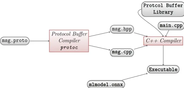
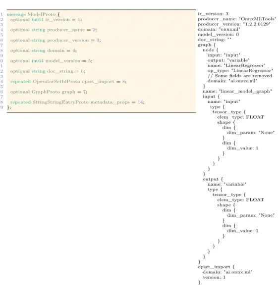
3.1 Process of producing C++ code from protocol buffer definition file and using it in a C++program to read ONNX file that represents ML model. 39 3.2 Snippet from ONNX proto definition of a top-level model container.

Right side shows textual representation of complete deserialized ONNX model. . . 41

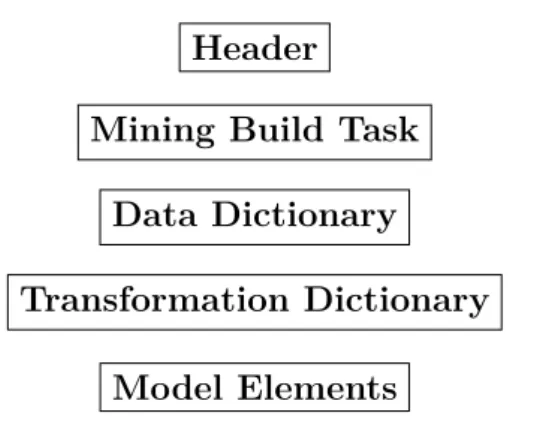
3.3 Structure of PMML model’s XML document. . . 44

4.1 Architecture of IL service daemon. . . 49

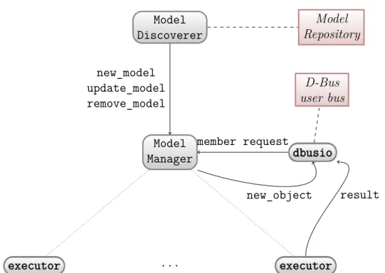
4.2 Actor model-based design of intelligence layer. Arrows represent

message sending. Dotted lines represent creation of executor actors by model manager. Dashed lines represent access to external resource like file system and D-Bus user bus. . . 54 5.1 Textual representation of input denotation for ResNet model’s input.

Left side is snippet that represents input of the graph. On the right side the key-value pairs of the ModelProto meta_data field are presented related to the IMAGE type. . . 57 5.2 Textual representation of output denotation for ResNet model’s output.

Left side is snippet that represents input of the graph. On the right side the key-value pairs in the meta_data field are presented related to CATEGORICAL_PROBABILITY type.. . . 58

5.3 Snippet from command line terminal showing the use of busctl and

the picture of cat that was used for testing. . . 59 5.4 Using IL service with D-Feet. . . 60

List of Tables

2.1 Common machine learning models for IoT. . . 21 2.2 Description of common machine learning models from Table 2.1. . . . 22 3.1 Libraries that claim to support ONNX format either internally or via

converters. . . 43 3.2 Models that are supported by PMML format. . . 45

(9)

Listings

3.1 Declarative MXNet code for training Rosenblatt’s perceptron with two synapses, for a binary classification problem using gradient descent method. . . 32 3.2 Imperative MXNet code for training Rosenblatt’s preceptron with two

synapses for a binary classification problem using gradient descent method. . . 34 3.3 Python code, showing how scikit-learn library can be used to train

linear model to predict closing price of Etherium crypto-currency based on the closing price of Bitcoin crypto-currency. . . 36 3.4 Snippet from protocol buffer definition of a ONNX Tensor. Used to

show basic constructs of PB message definition. . . 38 3.5 Definition of OperatorSetIDProto message, used to specify operator

set. . . 41

3.6 Snippet from XML Schema specification. . . 46 3.7 PMML document representing linear model for predicting closing prise

of Ethereum cryptocurrency based on the price of Bitcoin cryptocur-rency. . . 46 3.8 Python code to convert linear regression model to PMML file presented

(10)

government agencies [2] to develop strategic initiatives of applying AI in different domains, to create new types of intelligent systems, to provide new and improve current services, enhance and automate processes, and extract value from the massive amount of data that is being collected and stored in big datacenters all over the world. Internet of Things (IoT) is not an exception to the trend, especially considering massive amount of data that is forecasted by many to be produced by IoT devices and systems.

1.1 What is IoT today?

By reviewing the literature on IoT, it is difficult to form a clear and definite under-standing of what IoT represents, because the IoT concept is usually linked to some of its building blocks and not to the complete system of all required building blocks. Adding to the confusion are companies that are re-branding their products under IoT name for marketing purposes. [3]

Based on the definition of IoT provided in [3], the building blocks that form a conceptual framework of IoT are:

• Global connectivity infrastructure, like Internet network, that enables

con-nectivity and interoperability between computing devices.

• Physical objects or things, that are equipped with sensor and actuators, from the environment around us or on us, like assembly line on a factory floor, power grid, buses, cars, thermostats, light bulbs, mobile phones, watches, hearing aid equipment or household appliances, and their virtual representation in the cyber-space. These virtual representations are usually referred to as cyber-twins, digital twins or device shadows.

• Technologies that enable autonomy and self-management of things. It is

expected that the thing will continue to operate in the sensible manner even after connectivity to other things or global network infrastructure is lost or if one of the objects will start to malfunction. Self-management is the form of initial configuration and life-cycle management in terms of onboarding devices and receiving software updates without end-user interaction.

• Effective human-to-thing and thing-to-thing interfaces that allow physical things embedded with electronics to cooperate with other things, humans and virtual things located in cloud.

• Solutions that enable the coexistence and cooperation of heterogeneous compute devices and networking technologies.

• Services associated to things. For example, camera connected to Internet providing intrusion detection service or thermostat proving a service of heating

(11)

control and energy consumption optimization. The services might be combined so that thermostat can communicate to intrusion camera to detect the presence of the owner and adjust temperature accordingly. At the same time it might monitor the geolocation of owner by requesting location from owner’s phone or watch. This is an example of service composition in the application domain. The use-cases of IoT are smart homes, smart factories [4], smart electrical grids, smart cities and event smart labs [5]. IoT applied in the industrial or enterprise environment is usually named Industrial Internet of Things (IIoT) to differentiate it from consumer market IoT. Some of the use-cases have overlapping objectives. For example, the energy consumption optimization is crucial service throughout the domain of different human activities.

Tangible example of IoT related to smart city use-case are air quality monitoring

stations around Helsinki Metropolitan area Figure 1.1 (a). The information from

these sensors can be viewed by citizens during their subway trip to work or from the

Web using Web-Browser1_{. Another example, again from Helsinki Metropolitan area,}

are open APIs provided by Helsinki Regional Transport Authority (HSL in Finnish Helsingin Seudun Liikenne) that allow, among other things, to programmatically track real-time geolocation and other information about public transport on the

roads in Helsinki Metropolitan area Figure1.1(b). By using these APIs it is possible

to write application that gathers traffic data or allows user of the application to

make real time decisions like choosing an optimal route to work2_.

Staying with the smart-city use-case, major Finnish energy company Fortum is installing small mobile phone size devices to the households in the city of Espoo Finland that use AI based control system to ensure stable temperature in apartments

and make the heating more sustainable Figure 1.1 (c). The service provided by

Fortum also allows people, who have the device installed, to monitor humidity and temperature in their apartments using a Web-Browser or mobile phone application. All these activities are part of Fortum’s SmartLiving program.

One example of IIoT is open data access provided by Finnish national electricity transmission grid operator FINGRID. Near real-time time grid operation measure-ments are available in machine readable form. The list of all available open data is long, next only two representative examples are mentioned: frequency of the power

system, power production from different source of energy like nuclear or hydro3_.

Above real-world examples, that are in common use today, are all about collecting and presenting data from sensors connected to the Internet. But, as it was mentioned previously, IoT is not just a platform to collect and visualize data from different sources. It is also about, of what to do with the collected data, extracting valuable information out of it, using sensors measurements to achieve some goal and many other things that are presented in the list above. Every example of the use-case presented is prefixed with word smart, hinting that IoT systems are expected to be embedded with intelligence.

1_{More information available at} _{https://www.hsy.fi/en/residents/theairyoubreathe/}

Pages/default.aspx

2_{More information about APIs is available at}_{https://www.hsl.fi/en/opendata} 3_{Open data sets and APIs are available at}_{https://data.fingrid.fi/en/}

(12)

(b)

(c)

device

(a)

Figure 1.1: IoT use-cases around us: (a) Screen in the metro wagon showing air

quality report in Helsinki Metropolitan area. (b) Tracking of a bus in real-time.

Service provided by HSL. (c)Devices installed by Fortum as part of their SmartLiving

program, in apartment houses in the city of Espoo Finland.

1.2 Artificial Intelligence in IoT

One easy to understand application of artificial intelligence in IoT is Machine Learning (ML) applied to automated data analysis, also known under the name of data mining or big data. A challenging problem, that has a potential to be solved by IoT machine learning is collection of heterogeneous data from many different sensors and devices, all connected to the same global network connectivity infrastructure, turning data into valuable information from which long-term knowledge and proactive decision making can be deduced.

Until recently, the state-of-the-art approach of doing IoT machine learning was to collect data from the IoT devices, forward it and process it in the central cloud, either real-time or after data is collected. In other words, performing ML model training, historical analytics or real-time analytics in the cloud where data and compute power are highly available and distributed over many nodes. From the need to handle these large amounts of data, not always produced by IoT devices, emerged software for doing computation in such distributed systems like Hadoop and Spark and later followed extensions to those systems that enable applying machine learning in these highly distributed environments.

It was realized that the cloud approach is not applicable for use-cases where data-privacy, real-time actuation response, intermittent connectivity to cloud, bandwidth constrained data transport, are to be considered. Autonomous car would not send data to cloud for processing to decide does it see a red light or not, the latency is simply too high and will not allow the car to make a timely decision regardless of

(13)

the connection quality to the cloud. Also, it would not make sense to send all of the telemetry data generated by the car without any pre-processing, the volume is simply too great, and the value of sending all the data is usually not enough to justify bandwidth and storage capacity usage. That is the reason of why the current state-of-the-art in IoT machine learning is to combine massive capabilities of the cloud with the ability to pre-process the data already on the edge devices or do the inference based on the measurements locally. It might also be the case that security concerns or national regulation prohibit sending data for processing and storage to a cloud, hence making edge processing the most acceptable option. [6]

The data analysis applications, that are using machine learning techniques, are usually trained in the cloud or in the local computing infrastructure of developers and data scientists. After training and tuning process, the application is deployed to production environment, meaning edge device or a cloud compute instance using cloud-based management system or by some other means, for example integrating machine learning code into the application code.

How to distribute the intelligence so that it can be implemented in one environment and then deployed to various other environments is import subject that will be studied in this thesis.

1.3 Goals and Scope of the Thesis

In this thesis, the deployment of trained machine learning models to IoT devices is explored. IoT devices that are considered in this thesis are at least capable of executing Linux operating system. An example of such a device might be a mobile phone, IoT board with Intel processor for embedded applications or even a personal computer.

A prototype application was developed, in an attempt to decouple the code responsible for application logic like user interface from implementation of intelligence. The work is based on the concept of Intelligence Layer (IL) framework proposed in [7]. The prototype is called intelligence layer service. One of the tasks of intelligence layer, as presented in [7], is to provide intelligence as a local service to the applications

that need it. The concept of IL is not restricted to just being a platform for

serving intelligence to client applications, but in this thesis machine learning models’ description and serving aspects of IL framework are explored.

Decoupled trained ML model can be represented by a programming code in the form of a library or package for some specific programming language. Other approach is to have a compute instance in a central cloud, executing model code on HTTP request from the client program and replying with execution result. Third option is to use standardized Intermediate Representation (IR) format to represent a ML model. Special service will read a model file, turn it into runnable code and expose it to client processes via some Interprocess Communication Protocol (IPC). In this work, the third approach is explored.

Standardized IR format describes machine learning model in a library and platform independent way. Two state-of-the-art platform-independent model description

(14)

The main benefits from decoupling the intelligence from application using stan-dardized IR format, is to allow machine learning solution providers and data scientists, to use any existing machine learning library, that supports the standardized format, to develop their models and then export them in the standardized format to central model repository.

Users wanting to integrate the intelligence into their IoT environment production code, will be able to buy or download the model from the central repository and use it in their IoT environment to perform intelligent tasks. The user can use any machine learning library or runtime that is capable to translate standardized IR into library’s or run-time’s native IR format and execute the computations on a target device. This will allow the user to choose the computation platform that is most suitable for his task and compute requirements.

This approach has also a potential to make a deployment of machine learning models easier and democratize the machine learning space by not bounding model producers and consumers into specific libraries, run-times or cloud services. The approach can also allow model users to switch between different models and model providers if they choose to do so, without major changes to their code.

The major contribution and goal of this work is to study the possibility of decoupling the intelligence from applications and research state-of-the-art solutions that enable this decoupling.

1.4 Structure of the thesis

Chapter 2 and Chapter 3 provide a general background information related to

machine learning. Chapter 2 covers the theory behind artificial intelligence and

machine learning. It also has as subsection covering the most frequently used machine learning models in IoT data analyzing applications.

Chapter 3 presents practical aspects of machine learning like what state-of-the-art libraries are used to create machine learning applications and two current state-of-the-art formats for distributing machine learning models: Open Neural Network Exchange (ONNX) and Portable Model Markup Language (PMML). Some examples are provided showing how machine learning code, for simple ML problems,

looks like. It is assumed that reader is relatively familiar with Python and C++

programming language and examples are not explained in detail.

Chapter 4describes a prototype implementation of IL machine learning model serving concept. The software architecture of the IL service implementation is presented and implementation details of the architecture are explained.

In Chapter 5 results of using IL service implementation from Chapter 4 for serving computationally demanding image classification ML model are described. In the chapter a quick comparison between PMML and ONNX IR formats is provided and motivation for using ONNX as a model format for the prototype implementation is explained. It is also explained, how ONNX model must be modified in order to prepare it for successful provisioning to the device executing IL service.

(15)

2 Machine Intelligence and Machine Learning

Machine learning is a subset of AI techniques and methods for building artificially intelligent systems [8]. In recent years, one particular class of function-based ma-chine learning methods called deep learning was used successfully to solve artificial intelligence tasks that were difficult to solve using classical function-based machine learning techniques or other traditional model-based AI methods, like rule

based-or represent-and-reason methods [9, 10]. Solutions to problems related to object

recognition and localization in images or natural speech recognition were improved significantly by applying deep learning techniques, and new applications in different domains emerge all the time [11]. Even more impressive are combination of model-and function-based techniques as shown by current artificial champion AlphaGo in

the game of Go [10, 12]. These recent advances in AI created a lot of interest in

general public outside the scientific community, in research community, industry and government to apply machine learning and AI to various application domains.

In this chapter, fundamental ideas related to artificial intelligence and machine learning are presented. First, the concepts of machine intelligence and intelligent agent are considered. After that, it is presented how to formally specify machine learning problem. Some classical machine learning models and basic building blocks of a deep learning models are also covered.

2.1 Machine Intelligence

The original big goal of AI was to create a machine that is capable of achieving human level of intelligence, reaching the human’s level of performance in cognitive

tasks [10]. Machine Intelligence (MI) is limited AI. The objective of MI is not

to reach human level of intelligence, but to solve tasks that are considered intelligent. Classifying a piece of text as a funny story can be considered as machine intelligence. Many orders of magnitude more difficult task for a machine, of writing a funny story is outside of the scope of machine intelligence. Automation of tasks currently done by humans like controlling a vehicle in the real-world environment, doing customer support via phone or chat are also examples of domains where machine intelligence is in the process of being applied or is already part of the production service [13].

It is not easy to define machine intelligence precisely because definition of in-telligence itself is difficult. The Oxford English Dictionary defines inin-telligence as a faculty of understanding. The word faculty, in the context of intelligence, means natural or acquired ability to do something. Expanding the definition by including meaning of faculty one gets:

Intelligenceis natural or acquired ability to understand.

If in front of the definition above word machine is added, then it is better to replace word natural with intrinsic. There is nothing natural in computer program or current state-of-the-art electronic computing hardware created by humans. Natural things are created by nature. Things created by humans are artificial.

(16)

Living beings act based on their reflexes and understanding to survive, spread and achieve some objectives and machines can be programmed to do the same. Based on presented chain of reasoning the machine intelligence can be defined as:

Machine Intelligenceis an intrinsic or acquired ability of a computing machine or a computer program to understand and carry out actions to achieve objectives and

goals of its creator.

In the definition above, creator is considered to be a person or a group of people that designed and implemented machine intelligence. The intrinsic ability might be represented by a model or function suitable for a specific problem. The process of acquiring ability to understand is learning. Learning might represent fitting a curve to available training data or finding model parameters. The learned model can be used to perform an intelligent task.

The notion of intelligent agent is fundamental and useful mental tool for analysing and designing systems with machine intelligence capability [14]. Next subsection explains the notion.

2.2 Intelligent Agents

The term agent is used in many closely related areas of science and technology but doesn’t have a single universally accepted definition [15]. In [15] two views of agency are presented: a weak notion and a strong notion.

In a weak notion of agency, the agent is a software process or a combination of software and hardware that has the following four properties [15]:

1. Autonomy: agents have control over their internal states and actions and can operate without external interaction by other agents or humans.

2. Social ability: agents are capable of communicating with each other using some common communication protocol.

3. Reactivity: ability to understand their environment and ability to react to changes in the environment.

4. Pro-activeness: Agent can take an initiative and act preventively in order to achieve their goals.

For a stronger notion of agency, in addition to the properties from the weaker notion, agent is represented using concepts more applied to humans like knowledge, believe, desire and intention [15]. The stronger notion of agency is nearer to the big goal of AI as it was presented in the introduction to this chapter. Hence, for this thesis, a weaker notion of agency provides suitable scope for the work.

One other important property that is treated in the context of agent systems is rationality [15]. In popular university text book [14] about AI by Russell and Norvig, authors base their presentation of AI systems on the notion of rational agent. The general definition of an agent in [14] coincide with weaker notion of agency presented

(17)

in [15]. According to [14] agent is expected to: act autonomously, apprehend their environment, maintain persistency over its lifespan, adjust its behaviour according to changes in the environment, create and achieve goals. The rational agent is an agent as described in the previous sentence that acts to achieve its objective as well as possible [14].

In [8] instead of the agent the concept of artificial intelligent system that acts rationally is used. The system is rational if as a result of interaction with its environment it can take actions to maximize a long-term return.

In the description of an intelligent agent general concept like: actions, interaction, communication, environment, goals, objectives, long-term return were used. It is important to understand that when these concepts are discussed on the conceptual level, there is a lack of concreteness. For the specific machine intelligence problem, all these concepts become very concrete.

Let’s consider an imaginary problem from domain of predictive maintenance in petroleum industry, related to transporting gas over the pipelines lying deep on the seabed. The task might be to predict leaks in pipes and malfunctions in the gas pumping equipment to prevent natural disasters or to achieve a continuous operation and delivery. The environment is composed by sea, pipes, gas, equipment that enables operation of the whole system. The long-term objective of the agent is to prevent natural disasters and maximize continuous delivery of gas. The agent perceives the environment via the network of sensors scattered over gas delivery system. Actions of an agent imply to communicate to the human operator via computer screen or other digital means of communication that there is a high probability of an emergency situation. One other possibility is to place intermediate agents between agent that detect anomalies and human operators. One intermediate agent might suggest the optimal set of action that might trigger actions of the other agent that is a robot. The robot will go on-site to gather more information so that human operator can choose the best series of actions to maximize performance or mitigate the risks in timely manner. The agents must have a common protocol to communicate with each other and to the human operator.

The main task of rational agent is to map precept sequence to actions effecting environment in a way that maximizes performance measure. The percept sequences are obtained from sensors and actions are applied to environment via actuators. The agent is described mathematically via agent function. The agent function maps from

a set of percept sequencesS to a set of actions A:

f :S →A

The actuators and sensors are not necessary things that effect physical world

directly. They might be buffers in computer memory or sockets in a network

connection. The full description of performance measure, environment, actuators and sensors is called task environment. The machine intelligence problem is usually approached by first specifying task environment. The software implementation of agent function is called agent program. The computing devices with sensors, actuators

(18)

and system level software that form and execution environment for an agent program is called architecture. [14]

Currently the preferred method for creating agents is to create a learning agent [14]. One might even consider saying that it is impossible to implement machine intelligence systems in complex task environment without machine learning [8].

2.3 Machine Learning

Machine learning is mostly concerned with fitting a mathematical model to data and improving the model over-time using the observed evidence from the new data. Every component of an intelligent agent can be improved or implemented by using machine learning techniques [14]. The model might be represented by a function mapping inputs to outputs. In the introduction to this chapter, this approach is named the function-based machine learning. On the other hand, the model might contain some prior knowledge about the environment represented by probability distributions or general first-order logic. Probability theory and first-order logic are formal languages for describing environments. Machine learning techniques that

utilize these formalisms are called model-based machine learning techniques. [8,14,10]

In this thesis, only function-based machine learning models are considered. For a complete review of function- and model-based ML models reader can refer to classical text on AI like [14] by Russell and Norvig.

There are three principal types of machine learning: supervised, unsupervised and reinforcement [14]. The difference is best understood by considering three components that are required to formally specify the ML problem [8]. These components are:

1. Raw data points, features extracted from raw data points and labels related to data points.

2. Hypothesis space. 3. Loss function.

Data points are raw data precepted by an agent utilizing its sensors. The set

containing all possible values that can be assumed by a data pointz is denoted by

letterZ. The labels are answers to questions or predictions that the model gives as

output. Domain of all label value y, sometimes word target is used instead of label,

is denoted byY. Most often data points are pre-processed before they are given to

the model. As result of this pre-processing, data point is transformed into a vector

of features x, extracted from the data point. Symbol X is assigned to a space of all

the possible feature vectors. [8] Using the mathematical notation, the mapping from data points to labels can be represented by the following expression:

f :Z → Y (1)

What is referred to as a model is usually a mappingm:X → Y, hencef in 1can

(19)

The hypothesis space H is a set of all computationally feasible models that are

considered as candidates for the final modelm. Hypothesish, also called predictor

map, from H is usually a mapping from feature space X to label space Y. [8]

H={h(i) :X → Y|h(i)is computationaly feasible} (2)

In order to choose an optimal hypothesish that will be the final model m, from

hypothesis space 2, a measure of how good the model is performing is required. The

goodness of a hypothesis is evaluated using loss functionl 3. The loss function is

mapping from set-cross product of setsX, Y, H to real numbers R. The hypothesis

h that minimizes the average loss function is considered optimal and it is chosen as

final model m to make inferences.

l:X × Y × H →R (3)

Insupervised learning problems labeled data points (z(i)_{, y}(i)₎_∈

Z⊂ Z × Y are

provided by the hypothetical teacher. These labeled data points form a numerable

training set_Z. The job of the model creator is to find the best possible modelm∈ H

that is consistent on training data and generalizes well on new data points that are

not in _Z. Model is said to be consistent if it achieves near 100% accuracy over the

training set. Usually, it is not possible to achieve 100% consistency and get high prediction accuracy on new unseen data points. If the model is predicting accurately labels for data points that it has not used for training, it is said to generalize well to new data. If the model is consistent but does not generalize well to new data, it is said to suffer from over-fitting.

In unsupervised learning, only data points are providedz∈_Z⊂ Z. There are no labelled data points available. The job of the model is to group the data points based on some metric of similarity.

Inreinforcement learning, the model or agent learns by receiving reinforcements from the environment. Unlike in supervised learning, there is no teacher to provide correct labels to the model. Based on the input received from the environment model must decide how it should adjust itself in order to improve the performance. AlphaGo, current artificial champion in the game of Go, is an example of applying reinforcement learning problem to solve real world problem [12]. No human was able to beat the AlphaGo to date. In this chapter, only supervised and unsupervised learning models are considered.

Inputs and outputs of a model can be represented byquantitativeorqualitative

variables. Quantitative variables are measurable quantities represented by real numbers like pressure, voltage or velocity vector of a point. Note that quantitative variables are not necessary scalars. For example, velocity vector of a point in an open space is represented by three real number. Qualitative variables take values from a finite countable set of distinct elements. Elements of the set define categories.

For that reason, qualitative variables are also calledcategorical. An example might

(20)

The models outputting categorical labels are called classifiers and the models with quantitative labels are called regression models or predictors. Models that have both types of outputs are called mixed models [8].

For some machine learning classification problems that have by definition dis-crete label space the hypothesis space might contain mappings which map input to

continuous variable. The final prediction is then made using a decision function

that maps the values returned by hypothesis to labels. Ifd is decision function, then

f from1 can be rewritten as the following mapping composition:

f =fx◦m◦d

One more distinction exists between the machine learning models. They can be

parametric or non-parametric. Parametric models are described using a finite set of parameters. For example, if scalar value is predicted by the model that is represented by polynomial function, then coefficients are parameters. Knowing the coefficients, prediction can be calculated. Non-parametric models use feature vectors obtained from the data points to do prediction or classification.

The loss function 3 averaged over available feature vectors from _X is called

empirical risk, where_X is defined by:

X={(fx(z(i)), y(i))| (z(i), y(i))∈Z} (4)

The empirical risk is usually defined so that the main objective of machine learning algorithm is to minimize the risk. In mathematical terms empirical risk is a high dimensional function. Machine learning algorithm finds the best possible function from the hypothesis space, given observed data, that produces the global or local minimum of the high dimensional empirical risk function.

Now, that the basic theory of ML is covered, some common machine learning models used in IoT domain will be considered.

2.4 Machine Learning in IoT domain

The major use of machine learning in IoT domain is data analytics. In [16] an extensive evaluation and literature review of most frequently used machine learning techniques applied to data produced in the smart city environment was conducted.

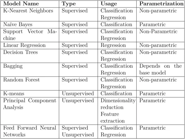
The result of this work is presented in Table 2.1. The table is modified from its

original form. As can be seen from the table, most of methods can be used for both classification and regression tasks and there are more supervised than unsupervised methods. This reflects the fact that supervised learning techniques are much more developed than unsupervised methods. Supervised methods are also more widely used in applications.

The first column of Table 2.1describes the name of the model. Second column

describes the type of machine learning: supervised or unsupervised. Third column describes is model used for classification or regression tasks. Note that most models

(21)

Table 2.1: Common machine learning models for IoT.

Model Name Type Usage Parametrization

K-Nearest Neighbors Supervised Classification

Regression

Non-parametric

Naïve Bayes Supervised Classification Parametric

Support Vector Ma-chine

Supervised Classification

Regression

Non-Parametric

Linear Regression Supervised Regression Non-parametric

Decision Trees Supervised Classification

Regression

Non-parametric

Bagging Supervised Classification

Regression

Depends on the base model

Random Forest Supervised Classification

Regression

Non-parametric

K-means Unsupervised Classification Parametric

Principal Component Analysis Unsupervised Dimensionality reduction Feature extraction Parametric

Feed Forward Neural Networks Supervised Unsupervised Classification Regression Parametric

can be used of both tasks. Fourth column describes, is the model parametric or non-parametric.

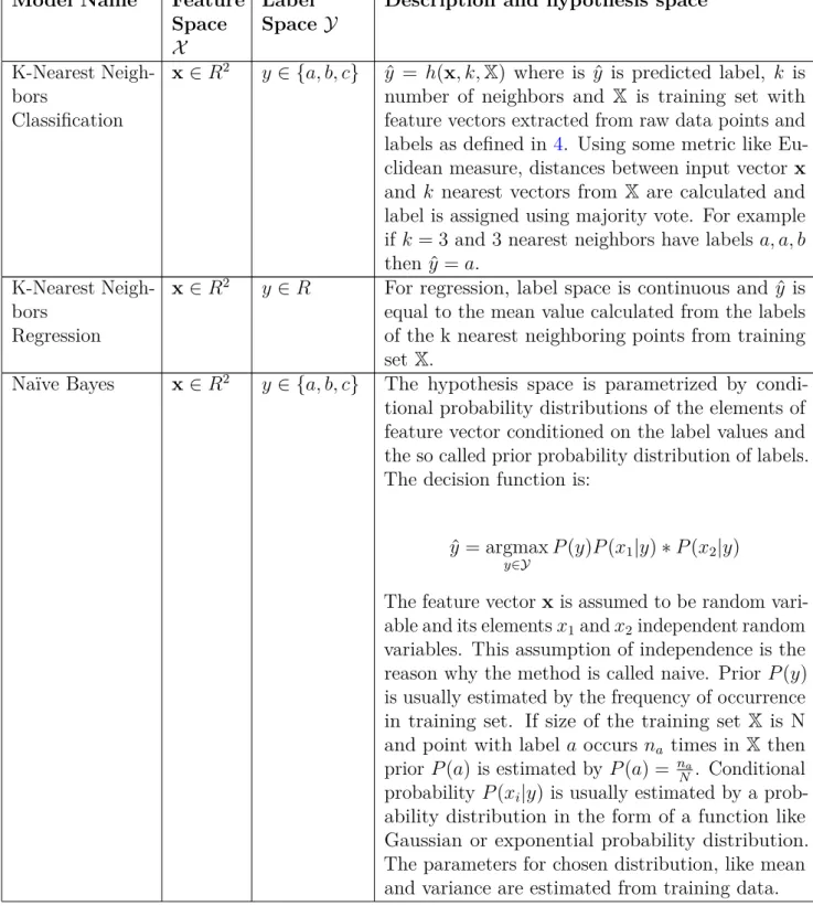
Table 2.2 shows typical feature space, label space and hypothesis space for

models presented in Table 2.1. Second column after the name column is for input

feature space. Third column describes output label space. Fourth column is a short description of model with mathematical description of its hypothesis space or decision function. Note that dimensions and elements of the spaces are picked randomly. The space of real numbers can be replaced by any other metric space. Metric space is set of elements that have a definition for a measure of distance between any two

elements from the set. The hypothesis spaces presented in Table2.2might not match

precisely with other formulation provided in the literature. Because neural networks are currently among the most popular machine learning methods, they are covered in more detail in next section. Next sections also shows how the concepts presented in Machine Learning section apply to the most basic type of neural network.

(22)

Table 2.2: Description of common machine learning models from Table 2.1.

Model Name Feature Space

X

Label Space Y

Description and hypothesis space

K-Nearest Neigh-bors

Classification

x∈R2 y∈ {a, b, c} yˆ = h(x, k,_X) where is ˆy is predicted label, k is

number of neighbors and _X is training set with

feature vectors extracted from raw data points and

labels as defined in 4. Using some metric like

Eu-clidean measure, distances between input vector x

and k nearest vectors from _X are calculated and

label is assigned using majority vote. For example

if k = 3 and 3 nearest neighbors have labels a, a, b

then ˆy=a.

K-Nearest Neigh-bors

Regression

x∈R2 _y_∈_R _{For regression, label space is continuous and ˆ}_y _is

equal to the mean value calculated from the labels of the k nearest neighboring points from training

set _X.

Naïve Bayes x∈R2 y∈ {a, b, c} The hypothesis space is parametrized by

condi-tional probability distributions of the elements of feature vector conditioned on the label values and the so called prior probability distribution of labels. The decision function is:

ˆ

y = argmax

y∈Y

P(y)P(x1|y)∗P(x2|y)

The feature vectorx is assumed to be random

vari-able and its elementsx1andx2independent random

variables. This assumption of independence is the

reason why the method is called naive. Prior P(y)

is usually estimated by the frequency of occurrence

in training set. If size of the training set _X is N

and point with label a occurs na times in X then

prior P(a) is estimated by P(a) = na

N. Conditional

probability P(xi|y) is usually estimated by a

prob-ability distribution in the form of a function like Gaussian or exponential probability distribution. The parameters for chosen distribution, like mean and variance are estimated from training data.

(23)

Support Vector Machine

Classification

x∈Rd _y_{∈ {−1}_,_1} _{Two class classification problem is provided as an}

example. This model can be extended to multi-ple classes using one-versus-rest formulation. The classifier is defined by:

h(x) =sgn(

n

X

i

αik(xi,x) +b)

Hereαare real numbers solved by the learning

algo-rithm using the training data. k is kernel function

defined by:

k(x,x0) =θ(x)·θ(x0)

Whereθis some vector valued function and·denote

vector dot product. Hence the classification

func-tion in hypothesis space depend on the choice of θ

and samples from training data. b is bias and sgn

signum function that returns 1 if input is positive

number and −1 if input is negative number. [17]

Support Vector Machine

Regression

x∈Rd _y_∈_R _{The hypothesis space for SVM regressor resembles}

hypothesis for linear regression with feature vector

replaced by θ(x).

h(x) = w·θ(x) +b

w vector and intercept b are learned from training

data. [17]

Linear regression x∈R2 y∈R The most basic technique for machine learning and

a text book favorite. The hypothesis is defined by

h(x) =w·x+b=w1x1+w2x2+b

The model is parametrized by weight vectorw∈R2

(24)

Decision Trees Classification Regression x∈R2 y∈R y∈ {0,1,2}

Decision tree learning algorithm partitions the fea-ture space into non-overlapping subspaces, it strat-ifies the feature space. For two-dimensional feature space in this example, the partition is easy to visu-alize with a figure. Figure I. below, shows recursive binary splitting of a feature space restricted to a

unit square [0,1]×[0,1]. Points in Figure I.

rep-resent samples from the training set. Color and shape of the points represent labels. Red circle is 0, green diamond is 1 and blue square is 2. Areas in

each strata form subspaces Ri. The splitting lines

are defined by values ti. [18]

t1 t2 t3 t4 R1 R2 R3 R4 R5 x2 x1 c1 = 0 c2 = 2 c3 = 2 c4 = 0 c4 = 0 Figure I.

For each region a simple model is fitted to the data. In the case of regression, it is constant calculated as a mean of all training samples inside the region. For classification decision tree the most dominating label among the training points in the region can be chosen as a label for the whole region. In Figure I classification problem is assumed. The dominating

labels are denoted by ci in the figure. [18]

The hypothesis space is composed of all possible partitions of feature space or its subspace. The hy-pothesis for the classifier and predictor estimating continues values have identical equations.

Equa-tion 5 depicts hypothesis map for partition

pre-sented in Figure I. I is a function that returns 1 if

xis inside region Ri and 0 if it doesn’t belong to

the region. [18] h(x) = 5 X i=1 ciI(x∈Ri) (5)

(25)

Decision Trees Classification Regression x∈R2 y∈R y∈ {0,1,2}

The decision tree is grown by recursively splitting the features space into non-overlapping regions. The technique is called decision tree because the hypothesis can conveniently be represented by a tree structure. [18]

Bagging Bagging is also referred to as bootstrap

aggrega-tion. In bootstrap aggregation the prediction of a hypothesis map of a base model is averaged over a collection of bootstrap samples with goal of reduc-ing the variance of estimation. [18]

If there is M bootstrap samples _X∗b _partitioning

the training set _X, the base model is fitted to each

sample getting the optimal base hypothesis map

m∗b_{. The final prediction is an average over base}

hypothesis maps [18]: h(x) = 1 M M X b=1 m∗b(x)

The above formula is for regression problem. For classification problem for each class indexed by

integer k the proportion of models pk(x)

predict-ing class k is calculated for data pointx. Bagged

classifier returns value that has the highest propor-tion. [18]

Random Forest Random forest model is a modification to bagging

with a decision tree as a base predictor. It con-structs a large collection of de-correlated trees and then averages the predictions from them to calcu-late final result like in bagging. The predictor map is similar to what was presented for bagging. The correlation is reduced by random selection of fea-tures from a feature vector at each step of growing a regression tree. [18].

(26)

K-Means x∈R2 _y_∈₁_{, ..., k} _{In k-means machine learning technique the}

algo-rithm clusters the points from training set into k

clusters, calculating the centroid for each cluster, using some similarity measure to determine which

point should belong to same cluster. k is

hyper-parameter representing the assumption about the

data. For the data points inR2_{the similarity might}

be Euclidean distance or the dot product of two fea-ture vectors. This method doesn’t require labeled data. Clustering can be interpreted as extreme case of classification problem when labels for the data points in training set are not available. [8]

The classifier function assigns a label to new input data point based on what centroid is nearest to the data point. The hypothesis space if formed by all possible cluster assignments and the decision functions might be:

h(x) = min(argmin

y∈Y

||x−my||)

Here, my are cluster centers. minfunctions picks

the class with minimal index. If distance

be-tween x and multiple centers is the same and

argmin||x−mk|| is a set that has more than 1

element then strategy is needed to choose only one

class, for that min is used. [8]

Principal

Com-ponent Analysis

x∈R13 y∈R2 Principal Component Analysis is used to reduce

the number of features in the high dimensional feature vector that is fed to machine learning model as input. Using high dimensional feature vectors requires a lot of compute and memory resources to execute the model. For some models using large number of features might produce an overfitting effect. Reducing the number of features to two is sometimes useful to visually inspect data. For these reasons reducing the number of feature is beneficial. [8]

The hypothesis map for PCA is linear

transforma-tion define by matrix W. For our example this is

13 by 2 matrix. How this matrix is calculated is out of scope for our work. Interested reader can read [8] to find out more about PCA.

(27)

Feed Forward Neural Networks

x∈R2 _x_∈_R _{A type of neural network without feedback loops.}

The hypothesis space is defined by network topol-ogy and a set of numerical parameters. The output

of a neural network is usually continuous. For

classification problem it can indicate the score or probability of belonging to different classes in a classification problem. Decision function for clas-sification problem picks the class that has highest probability.

Because of the current popularity of neural networks

they will be treated in more detail in section 2.5.

2.5 Neural Networks

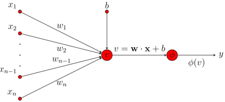
The most fundamental building block of any computational neural network is Rosen-blatt’s perceptron, named after a psychologist Frank Rosenblatt who published a paper presenting it in 1958. The perceptron represents a single unit of computation, that applies an affine mathematical operation and optional non-linear mathematical function to one or more scalar inputs producing a single scalar output. The percep-tron is a single neuron of a neural network, and a neural network is built out of such neurons with connected inputs and outputs. [19]

x1 x2 . . . xn−1 xn v b φ y w1 w2 wn−1 wn v =w·x+b φ(v)

Figure 2.1: Graph diagram of Rosenblatt’s perceptron.

Figure 2.1 illustrates Rosenblatt’s perceptron as a directed graph. Scalars xi,

where xi ∈ R, are inputs and can be thought of as components of m-dimensional

input vectorx ∈Rm_{. The directed arrows starting at inputs and converging at a}

single point are called synapses and a scalar number assigned to each synapse is

called a synaptic weight. One other converging arrow with bias value b is not part

of the input and is internal to the perceptron, it can be thought of as a translating component of an affine transformation. Using synaptic weights and bias perceptron

does affine transformation taking a dot product between input vector xand a vector

of synaptic weights wand adding bias b to the result. The result of affine operation

(28)

v =w·x+b

The nonlinear operation can be any real valued functionφ that takes local field as

input and produces final output of neuron. φ is also called activation function. Some

choices of activation function where found to be better than others for numerical stability and theoretical inferences like mathematical proofs. In practice only, couple of well-known and well-studied function are used for activation of a neurons. The symbolic mathematical expression for the perceptron is simply:

y=φ(v) =φ(w·x+b) (6) Rosenblatt’s perceptron can be trained to classify a linearly separable pattern in

a finite number of steps [19]. If a feature space is a subspace ofR2 _{and a label space}

consists of only two labels, the pattern is linearly separable if points belonging to different classes can be separated by a line. In higher dimensional space the line is a hyperplane.

Next, to highlight the basic concepts of machine learning presented in previous sections, an example of a perceptron that does binary classification of a linearly separable pattern in two-dimensional feature space is presented. It is assumed, that

the features are already extracted from the raw data and feature space isX =R2_.

Usually the process of identifying how to extract features and what features are import is quite involved process but it is skipped here, because it is a very domain

specific problem. The label space consists of two numberY = {−1,1}, number 1

identifies belonging to class C1 and number −1 to classC2. The model is described

by a neuron with two inputs and activation function is an identity. The decision function is a signum function that outputs positive one for positive value produced by a neuron and respectively negative one for negative number. The hypothesis space is parametrized by two weights and a bias values. For that reason, the hypothesis

space can be identified withR3_.

At this point: feature space, label space, model, hypothesis space and a decision function are defined. To train the model a loss function is needed, empirical risk and

training data. Discrete training set ofN training samples is denoted by_X. Elements

of this space are tuples (x(i), y(i)) where x(i) ∈ X and y(i) ∈ Y. The loss function

needs to be small when model classifies input feature vector correctly, indicating the correct prediction and the value of the loss function needs to be large when the model misclassifies the feature vector. For the example problem the following loss

functionl can be used:

l((x, y), h) = ln (1 +e−yh(x)) (7)

This function is called logistic loss function. The hypothesis map h is as in

expression6 with φ set to identity function. If the value of y is fixed to -1 and loss

(29)

when h is positive indicating the error in classification and it is decreases rapidly

whenh has negative values. If y is set to unity the effect is reversed. Plots for both

cases are presented in Figure2.2.

(a) l= ln (1 +eh₎ −4 −3 −2 −1 0 1 2 3 4 1 2 3 4 h l (b) l= ln (1 +e−h₎ −4 −3 −2 −1 0 1 2 3 4 1 2 3 4 h l

Figure 2.2: Logistic loss function7 as a function ofh fory=−1 in (a) andy= 1 in

(b).

The empirical riskEMRis an average of a loss function7over all samples from the

training set and can be expressed by the formula8. In this formula the mathematical

expression is expanded showing explicitly dependence ofEMR on elements of weight

vector w, bias b and training data from _X.

EMR= 1 N X (x(i)_,y(i)₎_∈ X l((x, y), h) = 1 N X (x(i)_,y(i)₎_∈ X ln1 +e−y(i)(w·x(i)+b) (8) = 1 N X (x(i)_,y(i)₎_∈ X ln

1 +e−y(i)(w1x₁(i)+w2x(i)₂ +b)

(9)

Now that all three components of a machine learning problem are specified the

model can be trained on the available training data. The loss function 7 has a

special property. It is differentiable with respect to hypothesis h. Since h is also

differentiable with respect to its parameters from the theory of calculus it is known that composition or sum of differential function is a differentiable function. Hence,

(30)

By minimizing the empirical risk with respect to parameters the best hypothesis,

that can be used for inference, is obtained. The parametersw and b that minimize

empirical risk are the ones that define the hypothesismthat is used to make inferences

after training. SinceEMRis differentiable function it is possible to find a critical point

of empirical risk function by equating is partial derivatives to zero as in equation 10.

Critical point can be local/global minimum, maximum or saddle point. Additional investigation must be performed in order find out the type of critical point. For function that are convex, like a parabola in two-dimensional Cartesian real space opening towards positive y-direction, the critical point is minimum but not necessary global minimum. ∂EMR ∂w1 = ∂EMR ∂w1 = ∂EMR ∂b = 0 (10)

The author presented the most simple type of feed-forward neural network con-sisting of only single neuron. Neural networks used for real world problems are much more complex utilizing other types of neurons that express for example convolution operation. These different types of neurons can form composite block called layer and layers can still be connected further forming very deep topologies. The outer layers are usually referred to as input and output layers, and inner layers are called hidden layers because they are not directly visible to the user of the network. Having many layers is the main reason why neural networks are called deep. Basically any network that has more than one hidden layer is considered deep.

Although in practice networks can be much more complex, as was explained in previous paragraph, the process of defining and training the network follows the same steps as presented for Rosenblatt’s perceptron. In the example presented, optimal weights and bias can be calculated analytically. For complex networks and other types of machine learning algorithms, it is usually near impossible to solve optimization problem of minimizing empirical risk analytically, that is why numerical methods must be used.

If empirical risk is differentiable the most popular methods of solving for optimal values are family of methods based on gradient descent. Gradient descent method is an iterative algorithm utilizing gradient of empirical risk to iteratively, step by step improve the estimate of a critical point. Gradient is vector field, the values of its components are derivatives taken at some point on the surface of empirical risk with respect to parameters and bias. Geometrically speaking empirical risk defines a surface in high dimensional space similar to equation of a sphere in 3-dimensional space. Being able to calculate derivatives is critical in utilizing gradient descent method and most of software for creating and training neural networks implement efficient data structures and algorithms for calculating gradients of complex function representing neural networks.

(31)

3 Machine Learning Libraries and Formats

In the beginning of this chapter two popular state of the art software libraries for creating, training and executing machine learning algorithms are presented. After that, two library independent formats for distributing machine learning models are considered. Because of the recent achievements of deep learning models [1], the most popular and hyped machine learning libraries are heavily specialized for creating, training and executing, data and computing hungry, deep learning architectures. Most of the libraries are available as open source software, but behind each popular deep learning library stands one of the IT industry giants like Facebook, Google or Amazon. Many deep learning libraries exist, only a few are mentioned next: TensorFlow (Google) [20], Caffe2 (Facebook), PyTorch (Facebook) [21], MXNet (Amazon) [22] and more exotic based on OCaml functional programming language

OWL [23].

One can classify deep learning libraries based on the programming model provided for defining computations to a software developer and data scientist. Currently, two programming models, also word paradigm can be used, exist: declarative approach and imperative approach. In Caffe2 library, data scientists can only use the declarative approach. In PyTorch, developers can only use the imperative programming model for writing ML code. MXNet supports both paradigms and for that reason it will be presented in this chapter, after the section about declarative and imperative approaches.

In this chapter classical machine learning Python library scikit-learn is also

presented. scikit-learn library [24] is scientific computation environment for doing machine learning and statistics calculations that can be considered a traditional imperative library for doing data-analytics and creating machine learning applications.

Common, to almost all machine learning libraries, is that they are partially

written in C, C++ or Fortran4, that is so called back-end implementation of the

library, for efficiency, but APIs for the users of the library are usually exposed via one or multiple other languages that are considered more convenient to use. Python being the most popular interfacing language at the time of writing this thesis.

After understanding how ML models are created, formats for enabling interop-erability between different machine learning libraries are covered. Interopinterop-erability is to be understood as having a common format for sharing ML models between different ML libraries. Two formats are presented: Open Neural Network Exchange (ONNX) [25] and Predictive Model Markup Language PMML [26]. The ONNX format will be used as a base for the proof of concept intelligence layer service prototype in later chapters of this work.

3.1 Differences between declarative and imperative approaches

In most state-of-the-art deep learning libraries, neural networks are represented by Directional Acyclic Graphs (DAGs) also called dataflow graphs. This is done to allow

4_{Mathematical libraries written in} _Fortran_{are still used for scientific calculations, especially}

(32)

efficient execution of neural network in training and inference and to make possible efficient calculation of partial derivatives by reverse mode algorithmic differentiation.

As was described in Chapter 2, the calculation of partial derivatives is a necessary

step for stochastic gradient descent, main technique used for training neural networks and other machine learning models when the loss function is differentiable.

In declarative approach to programming deep learning models, the compu-tational graph is defined before any computations take place. After the graph is defined, it is compiled into executable code and then used on every iteration either

for inference or training. The graph isstatic. The declarative approach is also often

described as define-and-run method orsymbolic approach to machine learning.

Imperative approach can be characterized by the phrase define-by-run,

no-tice theby in the phrase. The graph is constructed dynamicallyon every iteration.

This allows developer to use familiar style of imperative programming for constructing a graph, mixing construction of graph with control constructs of the host

program-ming language like conditionals: if, else and looping statements: for, while. It also

allows to get intermediate results of calculation much easier than with declarative approach.

The imperative approach is more flexible than symbolic approach. It allows to write and experiment with different deep learning parameter optimization techniques, variation of stochastic gradient descent for example, and network typologies much easier than with rigid static graphs. Declarative approach with static DAG allows for more performant code that can be parallelized and optimized for faster execution much easier than code written with imperative approach hence making training and inference faster.

Some libraries combine two approaches to benefit from both. For example, OWL

and MXNet use both techniques. In the code Listings3.1and3.2the author presents

MXNet code for training a one neuron perceptron classifier with two inputs and a

logistic loss function. The code in Listing3.2 is an example of imperative approach.

Code in Listing 3.1 is an example of declarative approach. Code for generating

synthetic training data is omitted from the listings.

Listing 3.1: Declarative MXNet code for training Rosenblatt’s perceptron with two synapses, for a binary classification problem using gradient descent method.

1 import mxnet as mx 2 import training_data 3

4 # Symbol represents matrix of feature vectors from training set. 5 x = mx.sym.Variable('x')

6 # Symbol represents vector of labels from the training set 7 # corresponding to feature vectors from x.

8 l = mx.sym.Variable('l')

9 # Symbol represents synaptic weights of the perceptron. 10 w = mx.sym.Variable('w')

11 # Symbol represents bias to the perceptron. 12 b = mx.sym.Variable('b')

13

(33)

15 v = mx.sym.broadcast_add(mx.sym.dot(x, w), b) 16 # Logistic loss function.

17 loss = mx.sym.log(1 + mx.sym.exp(-v * l)) 18 # Empirical Risk.

19 emr = mx.sym.mean(loss)

20 # Binding values from training data and initial values for synapses and ←

-bias.

21 ex = emr.bind(ctx=mx.cpu(), args={'x': mx.nd.array(training_data.X), 22 'l': mx.nd.array(training_data.y), 23 'w': mx.nd.array([[1], [1]]), 24 'b': mx.nd.array([1])}, 25 args_grad={'b': mx.nd.zeros(1), 'w': mx.nd.← -zeros((2, 1))}) 26 27 learning_rate = 0.1 28 for epoch in range(100):

29 # Calculating empirical risk and derivatives. 30 ex.forward(is_train=True)

31 ex.backward(mx.nd.ones(1))

32 ex.arg_dict['w'] -= learning_rate * ex.grad_dict['w'] 33 ex.arg_dict['b'] -= learning_rate * ex.grad_dict['b'] 34

35 print("Synaptic Weights")

36 w_final = ex.arg_dict['w'].asnumpy()

37 print("w_1 = {:.3}, w_2 = {:.3}".format(w_final[0,0], w_final[1,0])) 38 print("Bias")

39 print("b = {:.3}".format(ex.arg_dict['b'].asnumpy()[0]))

3.2 MXNet

MXNet is a library for creating large-scale deep neural networks. It is possible to do general mathematical computation with MXNet, but the library was designed to help developers to utilize the full computational capabilities of multiple GPUs and cloud compute infrastructure for creating neural networks. After-all, Amazon is the main stakeholder for the project. Library offers device placement to allow the developers to easily specify in what memory data structure used in computations are stored. For example, if computations are executed on the GPU then data structures must be in GPU’s memory and amount of copying between main memory and GPU memory must be minimal to avoid high latency when chucks of memory are moved

via slow external buses5. It is possible to scale computation over multiple GPUs

or network clusters. Library also provides automatic differentiation for calculating derivatives to optimize neural network’s parameters.

MXNet provides predefined neural network layers. These layers are optimized for speed. They can help developers to create efficient deep neural networks out of the ready-made building blocks without the need to write code for implementing common computations. For example, MXNet has predefined layer for fully connected

5_{External to CPU cache, GPU memory and main memory. That is buses which allow to move}