Multi-subject and multi-task experimental validation of the hierarchical
Bayesian diffuse optical tomography algorithm
Okito Yamashita
a,b,⁎
, Takeaki Shimokawa
a, Ryota Aisu
a,c, Takashi Amita
d, Yoshihiro Inoue
d, Masa-aki Sato
a aNeural Information Analysis Laboratories, ATR, 2-2-2 Hikaridai, Keihanna Science City, Kyoto 619-0288, Japan bBrain Functional Imaging Technologies Group, CiNet, 1-4 Yamadaoka, Suita City, Osaka 565-0871, Japan c
Nara Institute of Science and Technology, 8916-5 Takayama, Ikoma, Nara 630-0192, Japan d
Medical Systems Division Research and Development Department, Shimadzu Corporation, 1 Nishinokyo-Kuwabaracho, Nakagyo-ku, Kyoto 604-8511, Japan
a b s t r a c t
a r t i c l e i n f o
Article history: Received 28 December 2015 Revised 25 April 2016 Accepted 28 April 2016 Available online 3 May 2016Diffuse optical tomography (DOT) is an emerging technology for improving the spatial resolution and spatial specificity of conventional multi-channel near-infrared spectroscopy (NIRS) by the use of high-density measure-ments and an image reconstruction algorithm. We recently proposed a hierarchical Bayesian DOT algorithm that allows for accurate simultaneous reconstruction of scalp and cortical hemodynamic changes, and verified its per-formance with a phantom experiment, a computer simulation, and experimental data from one human subject. We extend our previous human case study to a multi-subject, multi-task study, to demonstrate the validity of the algorithm on a wider population and varied task conditions. We measured brain activity during three graded tasks (hand movement, indexfinger movement, and no-movement), in 12 subjects, using high-density NIRS and functional magnetic resonance imaging (fMRI), acquired in different sessions. The reconstruction perfor-mance of our algorithm, and the current gold-standard method for DOT image reconstruction, were evaluated using the blood-oxygenation-level-dependent (BOLD) signals of the fMRI as a reference. In comparison with the BOLD signals, our method achieved a median localization error of 6 and 8 mm, and a spatial-pattern similarity of 0.6 and 0.4 for the hand andfinger tasks, respectively. It also did not reconstruct any activity in the no-movement task. Compared with the current gold-standard method, the new method showed fewer false posi-tives, which resulted in improved spatial-pattern similarity, although the localization errors of the main activity clusters were comparable.
© 2016 The Authors. Published by Elsevier Inc. This is an open access article under the CC BY-NC-ND license (http://creativecommons.org/licenses/by-nc-nd/4.0/). Keywords:
Diffuse optical tomography Scalp bloodflow NIRS
Image reconstruction
1. Introduction
Functional near-infrared spectroscopy (fNIRS) is a noninvasive opti-cal imaging technique that measures the changes in oxygenated and de-oxygenated hemoglobin concentrations (hemodynamic changes) in response to changes in neuronal activity. fNIRS is sensitive to hemody-namic responses analogous to the blood-oxygenation-level-dependent (BOLD) signals found in fMRI, yet offers the advantages of low cost, easy portability, and the possibility of extending brain measurements to include such subjects as babies, elderly people, and patients with an implanted electronic device. It also permits measurements to be made
in ambient environments (for a historical review, seeFerrari and Quaresima, 2012).
The currently available fNIRS scalp topography methods have a cou-ple of disadvantages that reduce the reliability of the results when used as a brain imaging method. First, the relative positions of the measure-ment channels to brain anatomy vary between subjects, and also be-tween sessions within the same subjects. The activation foci consistently observed in the scalp topography do not necessarily indi-cate activation foci that consistently result from the same brain region. Second, fNIRS measurements are always affected by the hemodynamic changes in the scalp layer, and these changes may often dominate the contributions from cortical activity (Kirilina et al., 2012; Saager and Berger, 2005, 2007). Recently, one study showed that most of the oxy-hemoglobin concentration changes measured from the forehead during a verbalfluency task were due to changes in scalp hemodynamics (Takahashi et al., 2011). Several signal processing methods for the re-moval of scalp artifacts have been proposed, these include the use of principle component analysis (PCA) (Zhang et al., 2005), independent component analysis (ICA) (Kohno et al., 2007), adaptivefilters (Zhang Abbreviations:fNIRS, functional near-infrared spectroscopy; DOT, diffuse optical
to-mography; HbR, deoxygenated hemoglobin; HbO, oxygenated hemoglobin; LE, localiza-tion error; AUC, area under the receiver-operating curve; SS, spatial-pattern similarity; FPA, false positive amount.
⁎ Corresponding author at: Neural Information Analysis Laboratories, ATR, 2-2-2 Hikaridai, Keihanna Science City, Kyoto 619-0288, Japan.
E-mail address:[email protected](O. Yamashita).
http://dx.doi.org/10.1016/j.neuroimage.2016.04.068
1053-8119/© 2016 The Authors. Published by Elsevier Inc. This is an open access article under the CC BY-NC-ND license (http://creativecommons.org/licenses/by-nc-nd/4.0/). Contents lists available atScienceDirect
NeuroImage
et al., 2009, 2007), and short-channel regression (Gregg et al., 2010; Saager and Berger, 2005, 2007; Umeyama and Yamada, 2014; Zeff et al., 2007).
Diffuse optical tomography (DOT) is an emerging technology that may solve the above issues. It is a computer-assisted method for the three-dimensional reconstruction of images showing changes in cerebral hemodynamics. The technique uses a combination of high-density measurements, forward modeling, and an image reconstruc-tion algorithm (Bluestone et al., 2001; Boas et al., 2004; Eggebrecht et al., 2014). High-density measurements with an inter-probe dis-tance of around 10 mm allow multiple-disdis-tance channels and optical-path overlap between channels, which permits an increase in spatial specificity, in both the depth and surface directions. To ex-ploit this increased spatial specificity, a forward model that quantita-tively relates the activity inside the head tissue to the measured light intensity changes, is established by simulating a light migration pro-cess. An image reconstruction algorithm is then utilized to recon-struct a three-dimensional activity image from the observed light intensity changes. In principle, a reconstructed three-dimensional image allows for the separation and localization of scalp and cortical hemodynamic changes, improving the interpretation of results in terms of brain anatomy.
The quality of the reconstructed images depends on the image reconstruction algorithm, and a number of such algorithms have been proposed in previous studies. The image reconstruction problem is gen-erally formulated as a linear inverse problem (Arridge, 1999; Boas et al., 2004), which is an underdetermined problem requiring a priori infor-mation to constrain possible solutions. One scheme for solving the in-verse problem is the regularization approach, which uses a cost function consisting of the data fitting term and constraint terms representing a priori information (Boas et al., 2004; Cao et al., 2007; Culver et al., 2003; Lee et al., 2015). A DOT image is obtained by minimi-zation of the cost function. Another approach is to use Bayesian model-ing, which relies on a probabilistic model of observations and constraints called the likelihood function and prior distribution, respec-tively (Abdelnour et al., 2010; Guven et al., 2005; Shimokawa et al., 2012, 2013). A DOT image is obtained by computing the posterior bution and utilizing the representative statistics of the posterior distri-bution (e.g., mean or mode). The probabilistic modeling and posterior computation developed in the Bayesian statistics (Gelman et al., 2014) provide a systematic way to compute meta-parameters (e.g., the regu-larization parameter) in the algorithm. This allows established knowl-edge to be incorporated into models in a moreflexible manner.
Despite a variety of different image reconstruction algorithms, no re-search had proposed a DOT algorithm to accurately reconstruct both the scalp and cortical activity simultaneously, until we proposed the hierar-chical Bayesian DOT algorithm (Shimokawa et al., 2013). Currently, a two-step approach is used for real experimental data, including visual, auditory, and resting paradigms (Eggebrecht et al., 2014; White et al., 2009; Zeff et al., 2007). In this two-step approach, scalp artifacts are re-moved by short-channel regression, which is then followed by cortical image reconstruction using the depth-compensation minimum norm method (Culver et al., 2003). As an alternative, our hierarchical Bayesian algorithm simultaneously reconstructs activity in the scalp and cortical layers using an individual head model. The key concept is a probabilistic model characterizing the distinct nature of the scalp and cortical hemo-dynamic changes. We assume a spatial smoothness prior for the scalp hemodynamics and a sparse-promoting prior for the cortical hemody-namics. This is made on the basis of the empirical observation that scalp hemodynamics change globally (Funane et al., 2014; Kohno et al., 2007; Zhang et al., 2005), but task-related cortical hemodynamics change rather locally. We have previously verified the performance of our algorithm using a two-layer phantom experiment and a computer simulation (Shimokawa et al., 2013). This was followed by experimen-tal data from one human subject performing a rightfinger movement task (Yamashita et al., 2014).
In this work, we extend our previous human case study to a multi-subject and multi-task experiment, to test the validity of our algorithm on a wider population and different task conditions. A human case study demonstrated remarkable consistency between reconstructed cortical images and fMRI images (Yamashita et al., 2014); however, with con-sideration of inter-subject variability in light transmission and head anatomy, it remains unclear whether the previous single subject study can be generalized to a group level study. It is also unclear how our hi-erarchical Bayesian method performs with cortical activity of different sizes and amplitudes. To address these questions, we measured brain activity with high-density NIRS and fMRI acquired in different sessions, using 12 subjects, who performed three graded tasks. The three tasks were right hand movement, right indexfinger movement, and no-movement. These were selected to experimentally modulate the size and amplitude of the activations in the left primary motor cortex. We validated the performance of our algorithm using fMRI as a reference. In addition, we compared it with the two-step approach, which is the current gold-standard method for DOT (Eggebrecht et al., 2014).
1.1. Hierarchical Bayesian image reconstruction model
We originally proposed a hierarchical Bayesian sparse image recon-struction algorithm (Shimokawa et al., 2012), and later extended it to human functional brain imaging (Shimokawa et al., 2013). Here we briefly describe our model, while the image reconstruction algorithm is described in theAppendix A.
Wefirst reconstruct images of the absorption changes at multiple wavelengths, and then convert these to images of the hemodynamic changes (oxy- and deoxy-hemoglobin concentration) using spectral ex-tinction coefficients (Shimokawa et al., 2013, Eq. 13). Let x= (x1, x2,⋯, xN)tdenote the absorption changes in theNvoxels of the
discretized head tissue andy= (y1, y2,⋯, yM)t the log-ratio of the
light intensity changes measured by theMpairs of the source and detec-tor probes on the scalp. Under the condition that the absorption changes are small relative to the baseline condition, the Rytov approximation leads to a linear relationship between detected light intensity changes
yand absorption changesx (Arridge, 1999; Durduran et al., 2010; Shimokawa et al., 2012):
y¼Axþε; ð1Þ
where A is the sensitivity matrix andεrepresents the measurement noise. As absorption changes occur predominantly in the scalp and cor-tex where blood vessels exist, we assume measurements are affected by the absorption changes in these two layers. Thus Eq.(1)can be rewrit-ten as
y¼AcxcþAs
xsþε; ð2Þ
whereAc,xcandAs,xsare the sensitivity and absorption changes in the
cortical and scalp layers, respectively. Assuming measurement noiseε
follows a Gaussian distribution N(0, σ−1
Σ), the forward model (2) can be written as the following probabilistic model:
P yð ;xc;xs;σÞ N Ac
xcþAs
xs;σ−1Σ; ð3Þ
whereΣis a scale-normalized noise covariance matrix computed from the data during the baseline period, andσis the precision (inverse variance).
We assume the spatial smoothness and sparseness priors for the scalp and cortical absorption changes, respectively. For the scalp absorp-tion changes, we implemented the spatial smoothness prior by assigning high probabilities to the small values of the spatial derivative of absorption changeszsas follows:
zs¼Lxs; ð4Þ
whereLis the discretized version of the spatial Laplacian operator. A parameterη, which is determined from the data, controls the extent of the spatial smoothness. As the prior of the cortical absorption chang-es, locally extended activation is represented by sparse absorption changeszcconvolved with Gaussian smoothing operatorWas follows: xc¼Wzc ð6Þ P zð cjλÞ N0;Λ−1 ð7Þ Pð Þ ¼λ ∏ iΓλ i;λ0i;γ0 ; ð8Þ whereΛ= diag(λ),λ= (λ1,⋯,λNc) 'and Γðλ i;λ0i;γ0Þis the gamma distribution with meanλ0iand shape parameterγ0(assumed to be
com-mon to all voxels). The hierarchical prior distributions (7) and (8) pro-mote the sparseness ofzcby automatically adjusting all the elements of λ(called the relevance parameters) that control the amplitude range of absorption change in corresponding voxels (Faul and Tipping, 2002; MacKay, 1994; Wipf and Nagarajan, 2008).
Finally, a non-informative prior is assumed forσ,η to complete the full Bayesian formulation of our model:
Pð Þ η η−1
; ð9Þ
Pð Þ σ σ−1: ð10Þ
The image reconstruction algorithm determining all the parameters
xc,xs,σ,η,λfrom datay, can then be derived by inverting the above
model using the variational Bayesian method (Attias, 1999; Sato, 2001).
2. Methods 2.1. Subjects
Twelve healthy, right-handed males (22–45 years old) participated in the study. Written informed consent was obtained from all partici-pants before the experiments and they were paid for their participation. The experiments were conducted according to the Declaration of Hel-sinki and were approved by the Ethics Committee of the Advanced Tele-communication Research Institute International, Japan.
2.2. Subject tasks
All subjects participated in two experimental sessions conducted on different days; an fMRI experimental session was followed by a NIRS ex-perimental session (from 2 weeks to 4 months apart). In both the fMRI and NIRS experiments, each subject conducted three graded tasks: a right hand gripping task, a right indexfinger extension task, and a no-movement task (abbreviated as HAND, FINGER, and NO conditions). Subjects were instructed to rhythmically open and close their right hand in the HAND condition, to rhythmically extend their indexfinger in the FINGER condition, and to keep their hand still and relaxed in the NO condition. Throughout the experiment, subjects kept their eyes closed and listened to beep sounds delivered every second, the tones of which indicated the timing of the task movement and the rest period (high tone for task, low tone for rest). In one run, the subjects repeated one of the three tasks, as instructed at the beginning of a run. Each run commenced with a 10-second rest period, followed by 15 trials of the task period (15 s) interleaved with rest periods (20 s). In the rest period, subjects remained quiet with their arm still. All the subjects conducted two experimental runs of the three tasks, resulting in a total of 30 trials for each task. At the beginning of the NIRS session, the brain activity of subjects was measured during the resting-state (eyes closed) for 1 min.
2.3. NIRS data acquisition
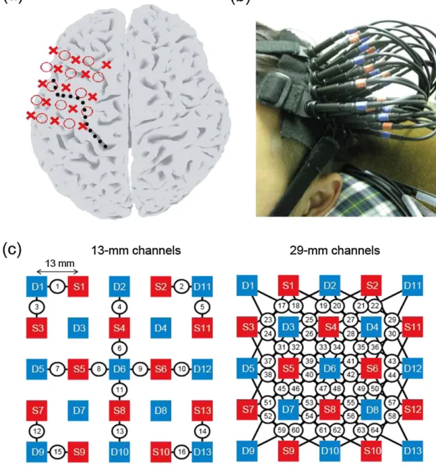
NIRS data were acquired using commercial NIRS equipment (FOIRE 3000, Shimadzu Corp., Japan) with electric amplifier gain and probe shape customized for high-density measurements. Using a custom-made holder, 12 source and 13 detector probes were placed on the left side of the scalp to cover the hand area of the primary motor cortex (Fig. 1(a) and (b)). We used a 5 × 5 square geometry, where thefirst and second shortest distances between source and detector probes were 13 and 29 mm, respectively. Because of a limitation with the mea-surement system, which only allowed for a maximum of 64 measure-ment channels, we recorded all the pairs of the second shortest channel (48 channels) and part of the shortest channel (16 channels; Fig. 1(c)). The sampling frequency was 5.3 Hz. For the co-registration of the NIRS data to the T1-MRI, the surface of the subject's face, three fiducial markers (nasion, left, and right preauricular points), and the positions of the probes, were all acquired using a hand-held laser scan-ner and a stylus marker (FastSCAN Cobra; Polhemus, USA).
2.4. MRI and fMRI data acquisition
Anatomical MR images were acquired for construction of individual head models, and functional images were acquired for evaluation of the reconstructed DOT images. All MRI images were acquired on a 3T Magnetom Trio Tim scanner (Siemens Medical Systems, Erlangen, Germany). T1-weighted anatomical images were acquired with an MPRAGE sequence (TR = 2250 ms, TE = 3.06 ms,flip angle = 9°, inver-sion time = 900 ms, FOV = 256 mm, matrix = 256 × 256, voxel size = 1 × 1 × 1 mm) and functional images were acquired using an echo pla-nar imaging sequence (TR = 3 s, TE = 30 ms,flip angle = 80°, FOV = 192 mm, matrix = 64 × 64, voxel size = 3 × 3 × 3 mm).
2.5. fMRI data processing
Activation maps from the three task conditions were derived using the general linear model implemented in SPM8 (http://www.fil.ion.
ucl.ac.uk/spm/software/spm8/). The image processing routine
consisted of head motion correction, followed by mass-univariate linear regression, with the task–rest contrast for each task and the head motion parameters, entered as independent variables. The resulting T-value maps were thresholded (pb0.05, FWE corrected) and percent signal maps for the three task conditions were also derived. The T-value maps and percent signal maps were then co-registered to each subject's T1 anatomical images and down-sampled to 4 × 4 × 4 mm voxels for comparisons with the reconstructed DOT images. As the anal-ysis was based on individuals' brains, we did not apply normalization to a standard brain.
2.6. NIRS data processing
The trial-averaged time series of the light intensity changes of the three wavelengths (780, 805, and 830 nm) were obtained from the raw continuous light measurement data using the following procedures:
1. Channels with a low voltage range were rejected (threshold: 5; num-ber of rejected channels: 2.8 ± 1.6 channels).
2. Voltage data were converted to log-ratios using a base-10 logarithm. 3. A digitalfilter was applied to each run data (low-pass: Butterworth filter of order 7, cutoff 0.3 Hz; high-pass: Butterworthfilter of order 3, cutoff 0.01 Hz).
4. ICA-wavelet motion artifact removal was performed on thefi l-tered data. Wefirst employed the logistic infomax ICA algorithm (binica.m in the EEGLab toolbox,http://sccn.ucsd.edu/eeglab/, Delorme and Makeig, 2004) to the data, which consisted of all the measurement positions and wavelengths (64 channels × 3
wavelengths). This resulted in an un-mixing matrix and indepen-dent component time series. The modified version of the wavelet motion artifact removal algorithm (Molavi, 2012; hmrMotionCorrectWavelet.m; with a parameter iqr = 3 in the HOMER2 toolbox,http://homer-fnirs.org/) was then applied to the independent component time series. Finally, the light inten-sity data were reconstructed by applying the mixing matrix (in-verse of the un-mixing matrix) to the processed independent time series. We applied the wavelet corrections to the independent time series, rather than the channel time series, to avoid correcting the time series of the three wavelengths independently.
5. Each run was segmented into trial data starting 8 s before the task onset and ending 35 s after the task onset.
6. The baseline of the data for each trial was adjusted to set the average amplitude during the pre-task period to 0.
7. For each of the three task conditions, outlier trials with a substantial deviation from the trial-median template were rejected (threshold: more than 2.5 × the variance in the whole time series, number of rejected trials: 0.5 ± 1.5 trials).
8. The trial data from each task condition were averaged.
The resulting trial-averaged light intensity data were then used as input to the DOT image reconstruction algorithms.
2.7. DOT forward model construction
The forward modeling consisted of head model construction, NIRS probe co-registration, photon migration simulation, and sensitivity computation. An individual's head model was constructed by segmenting their T1 anatomical image intofive tissue layers (scalp, skull, CSF, gray matter, and white matter) using FreeSurfer (http://
Fig. 1.High-density NIRS measurements. (a)Source and detector probes projected on a subject's cortical model. Circle and cross marks represent source and detector probes, respectively. Dotted line is the central sulcus along which the primary motor cortex is located. (b) Photograph of high-density NIRS measurement. (c) Channel configuration. Measurement channels consisting of source-detector pairs are represented by circles in the middle of the pairs (red: source, blue: detector).
freesurfer.net/). The NIRS probe positions were then co-registered to the head model using an affine transformation. The rotation and trans-lation parameters of the affine transformation were optimized so that a subject's facial surface, as measured by the laser scanner, matched that extracted from the T1 anatomical image. The photon migration process inside the head was simulated using Monte Carlo simulation software MCX (http://mcx.sourceforge.net/cgi-bin/index.cgi) with 109photons.
We used tissue optical parameters common to all three wavelengths (Table 1), as presented in a previous study (Fang, 2010). Finally, the sen-sitivity matrix, which related the absorption changes in the head tissue voxels to the light intensity changes at the source-detector pairs, was computed using Rytov approximation to the MCX results (Shimokawa
et al., 2012). For computation of the sensitivity matrix, the
1 × 1 × 1 mm voxel space was down-sampled to a 4 × 4 × 4 mm voxel space in the reconstructed images. The image reconstruction re-gion included the scalp and cortical voxels inside a 28-mm-deep cuboid, whose surface was a square along the scalp surface. This was obtained by extending the diagonals of the 5 × 5 NIRS probe square by a factor of 1.5.
2.8. Image reconstruction algorithm
For the image reconstruction, we followed the hierarchical Bayesian algorithm presented inShimokawa et al. (2013), with two important modifications that were necessary to make the algorithm work robustly on datasets with varying signal-to-noise ratios (see discussion for de-tails). Thefirst modification was the use of informative priors for the cortical activity instead of non-informative priors. The parameters of the hierarchical prior distribution were set so that the confidence pa-rameterγ0 was 5, and the mean parametersλ0iwere the mean square
values of the solutions obtained from the modified version of the depth-compensation minimum norm image reconstruction algorithm (see Appendix Afor details). The mean parameters were also used for the initial values in the algorithm. This setting allows for a slight biasing of the resulting sparse image towards a minimum-norm image that is ro-bust to low signal-to-noise levels. We set the confidence parameter
γ0= 5, on the basis of an empirical exploration of the values ofγ0= 0.01 , 0.1 , 1 , 5 , 10 , 100 and observations that the group-level quantita-tive evaluation was very similar forγ0= 5 , 10, 100, slightly inferior for
γ0= 1, and clearly inferior forγ0= 0.01 , 0.1. The second modification was an application of the approximation errors theory (Arridge et al., 2006) to absorb errors in forward modeling, such as probe co-registration error, tissue segmentation error, and photon migration sim-ulation error. An additional model error term was also introduced to Eq.(2), which followed the Gaussian distribution with a variance of 4 × 10⁻⁶for all the measurement channels, and for all the subjects.
The algorithm iterations were stopped when the relative change of the objective function (free energy) was lower than 10−6.
The modified depth-compensation minimum-norm algorithm for computing the initial value and the prior information of the hierarchical Bayesian algorithm required adjustment of two algorithm parameters: regularization and spatially-variant regularization. The regularization parameter, which controlled the balance between the datafit and the depth-compensation minimum-norm constraint, was automatically ad-justed by maximization of a statistical criterion called the marginal
likelihood (or type II likelihood). The spatially-variant regularization pa-rameter, which controlled the minimum sensitivity for depth-compensation, was set to an average sensitivity of around 20-mm depth from the scalp.
2.9. Image reconstruction evaluation
The reconstructed images were evaluated by comparison with the fMRI activation maps, which were considered as ground truth data. For evaluation of the DOT, the sign-inverted deoxygenated hemoglobin (HbR) images were used, rather than the oxygenated hemoglobin (HbO) images. This was because, in principle, the fMRI-BOLD signal varies according to paramagnetic agents, such as HbR (Ogawa et al., 1990), although some fMRI-NIRS studies showed empirical evidence that HbO-BOLD correlation was higher than HbR-BOLD correlation (Cui et al., 2011; Strangman et al., 2002).
The image reconstruction performance was quantified with four measures: the localization error (LE), area under the receiver-operating curve (AUC;Fawcett, 2006), spatial-pattern similarity (SS), and false positive amount (FPA). The LE signifies how well the main ac-tivity cluster in the fMRI is localized by the DOT. LE was computed as the distance between the center of mass of the main HbR activity cluster and the main BOLD activity cluster. We used a center of mass coordinate rather than a peak coordinate, as the localization error between two fMRI runs was smaller for the former case (mean values over all the sub-jects of 2.3 mm for the center of mass and 3.3 mm for the peak). AUC and SS indicate how well a spatial fMRI pattern is reproduced in the DOT. We computed AUC by regarding the fMRI T-map, thresholded at a p-value of 0.05 (FWE corrected), as the true binary image. SS was com-puted as the Spearman's rank correlation between the HbR image and the fMRI percent signal image. As computing LE, AUC and SS requires fMRI activations, these were evaluated for the HAND and FINGER condi-tions only. In addition, FPA was proposed to quantify spurious activation in a DOT image. The FPA was defined as the mean amount of negative HbR in the fMRI-null region (on voxels below the T-threshold). As the fMRI null region was defined using a positive T-value threshold, only negative HbR on fMRI-null voxels was averaged. The FPA allowed for quantification of the performance of the NO condition, where no fMRI activation was observed. Note that FPA was computed using HbR im-ages before sign-inversion so that increasing BOLD activations are com-pared with decreasing HbR responses.
2.10. Image reconstruction methods for comparison
For comparison purposes, three DOT images were computed for each dataset. Thefirst method used our hierarchical Bayesian algorithm mentioned previously (denoted as HB, hereafter). The second method was the modified depth-compensation minimum-norm algorithm (de-noted as MN), which was used as the initial value and prior information of the HB method.
The third reconstruction used the current standard method devel-oped in Washington University (denoted here as MN-WU), which has been previously validated using a variety of experimental datasets (Eggebrecht et al., 2014; White et al., 2009; Zeff et al., 2007). The NIRS process pipeline and image reconstruction algorithm presented in the supplementary materials ofEggebrecht et al. (2014)were followed. In
Table 1
Optical parameters in head tissue types (common to 780, 805 and 830 nm).
Tissue types Absorption coefficientμa(mm−1) Scattering coefficientμs(mm−1) Anisotropy (g) Refraction index (n)
Scalp & skull 0.019 7.8 0.89 1.37
CSF 0.004 0.009 0.89 1.37
Gray matter 0.02 9.0 0.89 1.37
brief, the NIRS process pipeline involved channel rejection, conversion to log-ratio, 0.01 Hz high-passfiltering, scalp artifact removal using global average of the short separation channel signals and regression, 0.3 Hz low-passfiltering, ICA-wavelet motion artifact removal, trial seg-mentation, trial rejection and trial-averaging for each task condition. The image reconstruction algorithm applied was the original depth compensation minimum norm algorithm (Culver et al., 2003), with the spatially variant parameterβ= 0.1 and the regularization parame-terαdetermined by the marginal likelihood of each data set (see Appendix A). A data-dependentαwas adopted, rather than afixed value ofα= 0.01, as presented inEggebrecht et al. (2014), as the depen-dent case was superior in the group-level performance evaluation. The reconstructions were constrained to all voxels in either the scalp or cor-tex (Eggebrecht et al., 2012).
3. Results 3.1. fMRI results
To determine the reliability of the activation maps used as ground truth data, wefirst evaluated the consistency of the activation maps be-tween runs 1 and 2. For the HAND condition, the reproducibility of the left M1 activity, as measured by the Pearson correlation, was very high for all the subjects (0.88 ± 0.07). For the FINGER condition, the repro-ducibility was very high (0.78 ± 0.11), except for one subject who showed almost no activity in one run, resulting in a low correlation co-efficient of 0.11. We therefore excluded this subject from the evaluation of the FINGER condition. For the NO condition, none of the subjects showed any significant activity (pb0.05, FWE corrected) in either run. With consideration of these results, we combined the data of runs 1 and 2, to obtain one activation map for each task condition for the DOT image evaluation. The sizes of the above threshold clusters in the HAND and FINGER conditions were 3472 ± 1582, and 1389 ± 1288 mm3, respectively, and the largest T-values of the M1 activities
were 27.3 ± 5.1 and 17.4 ± 3.9, respectively.
3.2. NIRS results
The trial-averaged HbO and HbR data, measured with 13- and 29-mm channels for the HAND condition of subject 12, are plotted in Fig. 2. With the 29-mm channels, sensitive to cortical activity, task-related waveforms typical of those observed in the fMRI block paradigm were localized to the middle to posterior channels. On all the 13-mm channels, in which the sensitivity was dominated by scalp activity, non block-like waveforms were observed. We found uniformity of waveforms on the 13-mm channels in most of the datasets, including the NO condition. The PCA analysis of the continuous light intensity data from the 13-mm channels revealed that in 69 out of 72 runs (12 subjects × 6 runs), thefirst principal component explained more than 50% of the variance and more than one uniform index (Kohno et al., 2007), indicating that scalp activity was uniform rather than localized.
3.3. DOT results
We evaluated the reconstruction performance of the DOT algorithms by comparing the cortical HbR DOT images with the fMRI activation im-ages. Wefirst demonstrate the qualitative evaluations by plotting the DOT images and the DOT time series for one representative subject (subject 12) and then show a quantitative evaluation that summarizes the data from all the subjects. The cortical HbR-DOT images of the re-maining 11 subjects and examples of HbO-DOT images are presented in the supplementary material.
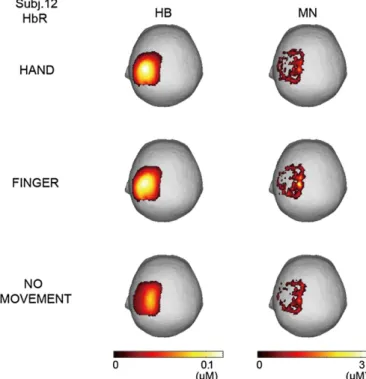
The cortical HbR images reconstructed using the three DOT methods are plotted inFig. 3, along with the fMRI T-value images. For visualiza-tion purposes, voxel based images were mapped onto the cortical sur-face using inverse distance weighting interpolation. All of the DOT
images were computed as average activities within a time window from 5 to 25 s after the task onset. The HbR images reconstructed using the HB method were consistent with the fMRI T-maps in all the conditions. The MN and MN-WU methods also succeeded in reconstructing the main cluster of activity along the central sulcus, with a similar accuracy to the HB method. However, spurious activities, which were not observed in the fMRI T-maps, were also reconstructed. Even in the NO condition, where no significant fMRI activity was ob-served, the MN and MN-WU methods reconstructed activity with an amplitude comparable to the HAND condition. This was because the depth-compensation property artificially enhanced the amplitude of deep activity, or activity on the edge of the reconstructed region. The LEs of the HB, MN, and MN-WU methods were 3.0, 5.4, and 6.2 mm for the HAND condition, and 8.0, 9.0, and 7.0 mm for the FINGER condi-tion. The AUCs of the three methods were 0.92, 0.83, and 0.82 for the HAND and 0.82, 0.71, and 0.69 for the FINGER condition. The SSs of the three methods were 0.82, 0.70, and 0.72 for the HAND and 0.69, 0.47, and 0.44 for the FINGER condition. The FPAs of the three methods were−0.18,−0.47, and−0.45 for the HAND,−0.18,−0.42, and −0.40 for the FINGER and−0.007,−0.12, and−0.05 for the NO con-dition. The cortical HbO images resembled sign-inverted HbR images (see supplementary materials).
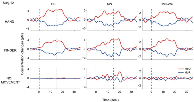
The time series of the cortical HbO and HbR concentration changes at the peak voxel are presented inFig. 4. In the HAND and FINGER condi-tions, all three methods successfully reconstructed positive HbO and negative HbR changes, with durations of around 20 s, and onset delays of 5–7 s. This is indicative of the wash-out mechanism, which is consid-ered to be the origin of task-related BOLD signal changes. In the NO con-dition, the HB method reconstructed images without activation, while the MN method resulted in activity patterns comparable to the HAND condition. The MN-WU method also resulted in some small false posi-tive activity.
Scalp HbR images are plotted inFig. 5. These images were com-puted by taking the root mean square values from the voxel-based images, within a time window from 5 to 25 s, and converting the values to the scalp surface images. The scalp image from the HB method is smooth; however, the MN image is less so and tends to have large values around the edge of the reconstructed region. The scalp HbO image showed the same tendency (see supplementary materials). The spatial smoothness of the HB reconstruction is not merely due to the prior information, as the parameter controlling smoothness was adjusted from the data.
InFig. 6, the time series of the scalp HbO and HbR concentration changes for the four voxels just beneath probes D1, D9, D11, and D13 (Fig. 1) were plotted for the HB and MN methods. The scalp time series from one representative channel (channel 6), which was identified from the global average of the 13-mm channels, was plotted for the MN-WU method (all the 13-mm channels had identi-cal sidenti-calp waveforms, but with different amplitudes). The temporal patterns resulting from the HB method showed little spatial variabil-ity, whereas those of the MN method were highly inhomogeneous. In particular, the waveforms of the D13 voxel (right-bottom panels), which were reconstructed using the MN method for the three task conditions, appeared random because of the influence of measure-ment noise from the nearby 30-mm channels. Conversely, the HB method was less influenced by measurement noise, and the recon-structed HbO waveform showed similarity with the scalp waveform identified from the global average of the 13-mm channels. However, we observed a discrepancy between the reconstructed HbR wave-form and the scalp HbR wavewave-form of the global average of the 13-mm channels. Two possible causes for this discrepancy are reduced accuracy of the scalp HbR reconstruction due to modeling error, and the influence of cortical contributions on the global average of the 13-mm channel.
We evaluated the reconstruction performance using four quantita-tive measures, LE, SS, AUC, and FPA (Fig. 7). We excluded any DOT
images that all three methods failed to reconstruct. We judged a method as a failure when one of the following three conditions was satisfied: an LE exceeding 15 mm, an AUC at chance level, or an SS at chance level. With these criteria, none of the 12 subject reconstructions failed in the HAND condition, but two of the 11 subject reconstructions failed in the FINGER condition. Compared with the MN and MN-WU
methods, the HB method achieved comparable LE scores, and signif-icantly better SS and AUC scores in the HAND condition, while per-formance was better overall in the FINGER condition (Wilcoxon's sign rank test). The HB method achieved the best FPA scores for all the conditions. These results were consistent with the results of the qualitative evaluation of the cortical DOT images (Fig. 3 and Fig. 2.Representative example of high-density NIRS data from subject 12 and the HAND condition. Trial-averaged HbO (red line) and HbR (blue line) waveforms of the 13-mm (a) and 29-mm channels (b) are plotted in each panel located on the center of corresponding source-detector pairs (seeFig. 1(c)). Two vertical lines inside each panel indicate task onset and offset. A = anterior, P = posterior, M = medial, L = lateral.
supplementaryfigures), where all three methods localized the main activity clusters, but the MN and MN-WU methods tended to also re-construct false positives. The median scores of the four measures are summarized inTable 2.
Finally, we investigated the quantitative relationship between the reconstructed HbR and BOLD signal changes. We summated the (sign-inverted) HbR concentration changes and BOLD percent signal changes, of the main cluster of activity for each subject. The relationship was quantified by examining the Pearson correlation between the HbR and
BOLD across subjects. For the HAND and FINGER conditions, the HbR change reconstructed using the HB method showed the greatest pro-portionality to the BOLD signal changes, as shown inFig. 8. The cross-subject correlation coefficients for this method were 0.82 and 0.69 for the HAND and FINGER tasks, while those of the MN and MN-WU methods were less than 0.5 in both tasks. No quantitative relationship for the NO condition was expected, as the main clusters of activity in the fMRI and DOT techniques were not located in corresponding regions.
Fig. 3.Cortical activation maps of fMRI T-value and reconstructed HbR concentration changes from subject 12 in the three task conditions. In fMRI T-maps, activity over the threshold T = 5.35 (p = 0.05, FWE corrected) is shown. The three HbR images are averaged over a time window from 5 to 25 s after task onset. Only the left hemisphere is shown.
Fig. 4.Time series of reconstructed cortical HbO/HbR concentration changes at the peak voxel on left primary motor cortex in subject 12, for the three task conditions. In each panel, reconstructed HbO/HbR time series (red/blue lines) are plotted. Vertical dotted lines represent task onset and offset. The same y-range is used across task conditions.
4. Discussion
We report on the multi-subject and multi-task experimental valida-tion of our HB DOT image reconstrucvalida-tion algorithm, using fMRI as a ref-erence. We also compared the HB algorithm with the current standard MN-WU method for DOT image reconstruction (Eggebrecht et al., 2014). Compared with this current standard method, the HB showed
fewer false positives, which resulted in greater spatial-pattern similari-ties with the fMRI results, although differences in localization of the main peak activities between fMRI and DOT were comparable for both DOT reconstruction techniques. Additionally, the HB method achieved substantially greater cross-subject correlation between the total quanti-ty of HbR change and the total BOLD signal percent change, indicating it was quantitatively more reliable. Compared with the BOLD signals, the HB achieved an LE of 6 mm and an SS of 0.6 for the HAND condition, and an LE of 8 mm and SS of 0.4 for the FINGER condition. The HB algo-rithm did not result in any significant activity in the NO condition, a con-dition that was expected to result in an absence of activity. We also confirmed the HB reconstruction performance did not degrade using only two wavelength data which most of the commercially available fNIRS/DOT systems employ (see supplementary).
A comparison with the current standard method of DOT reconstruc-tion revealed performance improvements with the HB algorithm. The HB method is different from the standard method in two main respects. First, the HB method simultaneously reconstructs scalp and cortical ac-tivities within the DOT framework, whereas the standard method re-constructs cortical activity using a two-step method where the scalp contribution is removed by the short-channel linear regression, follow-ed by image reconstruction of the cortical activity. This two-step meth-od may cause problems when the distance of the short-channels is not sufficiently short. In this case, the shortest channels will be sensitive to part of the cortex, and the short-channel linear regression method will remove not only the scalp activity, but also part of the cortical activ-ity. In our dataset, in four of the 12 subjects, the 13-mm channels had a not insignificant cortical sensitivity (more than 10%). Second, the HB method uses a sparse-promoting prior for prior information on cortical activity, whereas the standard method uses a depth-compensation L2-norm minimum L2-norm prior. The sparse-promoting prior provided more focused cortical DOT images than the standard method; the stan-dard method's depth-compensation is sometimes problematic as it arti-ficially increases the amplitude of voxels with low sensitivity. With the MN-WU method, we frequently observed large activations in voxels near the boundary of the estimated region. These were not observed Fig. 5.Scalp activation maps of reconstructed HbR concentration changes from subject 12
in the three task conditions. Each HbR image is the root-mean-square image over a time window from 5 to 25 s after task onset.
Fig. 6.Time series of reconstructed scalp HbO/HbR concentration changes from subject 12 in the three task conditions. First and second columns show scalp HbO/HbR waveforms (red/blue lines) from four scalp voxels just beneath the four probes D1, D11, D9, and D13, reconstructed by the HB and MN methods. The third column shows the scalp HbO/HbR waveforms from one representative channel (channel 6) removed by the short-channel regression in the MN-WU method. Vertical dotted lines represent task onset and offset. The same y-range is used across task conditions.
in the fMRI images and less frequently in the HB-DOT images (see sup-plementaryfigures).
We added two important modifications to the HB algorithm that was described in our previous studies. These were to improve the ro-bustness of the algorithm to datasets with different signal-to-noise ra-tios. The first modification was to use informative priors for the cortical activity, instead of (nearly) non-informative priors, which were used in the previous simulated data and single human case study. In the previous studies, we used a non-informative prior by set-ting the confidence parameterγ0to 0, or a very low value. This setting resulted in accurate sparse DOT images when the signal-to-noise ratio of the data was high. However, in this study we observed incorrectly lo-calized sparse DOT images in some subjects when the data had a low signal-to-noise ratio. To resolve this issue, we adopted the informative prior, which slightly biases the resulting sparse image to a depth-compensation minimum-norm image that is more robust to low signal-to-noise ratios. The value ofγ0determining the balance between the data and the prior information is an important parameter affecting the reconstructed images. Although we used a common parameter for all the subjects, it would be interesting to determine the optimal value for each subject and dataset, to facilitate optimal reconstruction of each individual DOT image. We did attempt to determine the optimal value using statistical criteria such as free energy, model evidence and
DIC (Gelman et al., 2014); however, we failed tofind a technique for de-termination of the optimal parameter, even for the simulated data. De-termination of the optimalγ0value is still a problem requiring further work.
The second modification was adoption of the approximation er-rors theory (Arridge et al., 2006) to absorb errors in forward model-ing. In some subjects, we observed waveforms resembling sign-inverted cortical waveforms in the reconstructed scalp activity. This happened because the algorithm put too much emphasis on fitting to data from the 13-mm channels, as the noise variance of these channels, which was estimated from thefluctuations of the pre-task period, was too low. Such excessively low variance in the 13-mm channels is not problematic if there are no error factors in the forward modeling. However, in the real experimental data, sev-eral error factors were found, such as probe co-registration, tissue segmentation and photon migration simulation errors. If these error factors are not taken into consideration, the noise variance of the 13-mm channels may be underestimated, and cause overfitting of the 13-mm channel data by adjustment of scalp absorption change. To avoid this phenomenon, we introduced an additional model error term to Eq.(2), which follows the Gaussian distribution, based on the approximation error theory. In this study, we deter-mined the variance from a single subject's data value as 4 × 10⁻⁶,
by observing the sign-inverted cortical waveforms in the scalp layers, while gradually increasing the value, and selecting a value when the sign-inverted cortical waveforms disappeared. Although the optimal model error variance may differ between subjects, we applied the same value to all subjects. Determination of the model error variance in an objective and systematic way is a practically im-portant problem for future work.
Whether our spatial smoothness assumption for scalp activity is generalizable to other NIRS experiments requires further experimental evidence. Our short-channel PCA analysis revealed the homogeneity of scalp activity above the left primary motor cortex, regardless of the task conditions. Several previous studies have supported thefinding of spatial smoothness in scalp activity in the motor and visual cortexes (Gregg et al., 2010; Kohno et al., 2007; Zhang et al., 2005). However, Fig. 7.Group-level reconstruction performance evaluated using four quantitative measures: LE, SS, AUC and FPA (from top to bottom rows). In thefirst and second columns, distributions of the four measures for HAND (all 12 subjects) and FINGER conditions (9 subjects) are shown using boxplots. In the third column, FPA for the NO condition (12 subjects) is shown.
Table 2
Summary of the group-level quantitative evaluation (median and mean absolute deviation). HB MN MN-WU HAND LE 5.9 ± 2.4 7.0 ± 3.7 7.6 ± 3.1 SS 0.62 ± 0.12 0.38 ± 0.15 0.47 ± 0.19 AUC 0.86 ± 0.04 0.79 ± 0.09 0.81 ± 0.13 FPA −0.31 ± 0.13 −0.63 ± 0.19 −0.49 ± 0.10 FINGER LE 7.8 ± 2.2 7.9 ± 2.4 7.1 ± 3.2 SS 0.42 ± 0.16 0.29 ± 0.10 0.38 ± 0.13 AUC 0.84 ± 0.04 0.71 ± 0.11 0.78 ± 0.13 FPA −0.21 ± 0.04 −0.80 ± 0.25 −0.46 ± 0.12 NO FPA −0.005 ± 0.005 −0.16 ± 0.09 −0.13 ± 0.05
in one paper the authors reported inhomogeneity of the scalp activity around the left motor cortex during afinger tapping task (Gagnon and Cooper, 2012). The prior information used for scalp activity should be revised with accumulated experimental evidence.
Evaluation of the whole procedure of image reconstruction, which consists of forward modeling and the image reconstruction algorithm, is a difficult problem. We focused on evaluating the latter reconstruc-tion part in this study. How different parts of the forward modeling such as tissue segmentation methods, sensitivity computation methods and use of the standard brain (Custo, 2010; Ferradal et al., 2014) affect image reconstruction performance requires investigation. In particular, optimization of the whole procedure, taking both accuracy and time into account, is essential to make the DOT technology practically useful (Dehghani et al., 2008; Jermyn et al., 2013).
In summary, this study showed the feasibility of applying our HB al-gorithm to wider subject populations and wider task conditions. It also demonstrated its superiority over the standard DOT algorithm. We are now investigating applicability of our algorithm to brain network studies.
Acknowledgments
This research was supported by a contract from the National Insti-tute of Information and Communications Technology entitled‘ Develop-ment of network dynamics modeling methods for human brain data simulation systems’(grant # 173) and the ImPACT Program of the Council for Science, Technology and Innovation (Cabinet Office, Govern-ment of Japan).
Appendix A. Image reconstruction algorithm
This appendix describes the image reconstruction algorithm used in this study. Note that the algorithm below considers one wavelength for simplicity.
The following mathematical notations are used. Thei-th element of a vectorx,ii-th element andi-th row of a matrixXare denoted by (x)i,
(X)iiand (X)i⋅, respectively. The transpose of a vector xis denoted by x′. An operator diag(x) denotes a diagonal matrix whose diagonal ele-ments are given by (x)i. An operator meantxtdenotes mean ofxtwith
respect tot. A dot productx.∗ydenotes an element-wise multiplication of two vectorsxandy. The identity matrix is denoted byI.
In the following we use the variables defined in the "Hierarchical Bayesian image reconstruction model" section. We further define the partition of imagexand sensitivityAto scalp and cortical voxelsx= [xs,xc] ,A= [AsAc], andItask: an index set of time points during task,T: the number of time points during task,Ns,Nc: the number of scalp and cortical voxels, respectively.
A.1. Depth compensation minimum norm
The MN-WU image reconstruction algorithm is briefly described, and follows the supplementary materials ofEggebrecht et al. (2014).
An MN-WU DOT image is obtained by minimizing the following cost function with the depth-compensation regularization:
Eð Þ ¼x ðy−AxÞ0ðy−AxÞ þαx0D 1x D1¼diagðρ1þβÞ ρ1 ð Þi¼ A0A ii
To avoid overcompensation for near-zero-sensitivity voxels, the spatially-variant regularizationβwas set to 0.1. Minimization of the cost function leads to an MN-WU DOT image as
xMN−WU¼ A0AþαD1− 1
A0y:
For a measurementy(t) at time pointt, we obtain a DOT imagexMN− WU(t). The regularization parameterαis automatically determined by maximizing the marginal likelihood using all the measurements Fig. 8.Quantitative relationship between total HbR (sign-inverted) and BOLD signal changes in main activity clusters across subjects. Total HbR changes of main activity clusters reconstructed by the HB, MN and MN-WU methods are plotted against total signal percent changes of BOLD signals for the task conditions, HAND, FINGER, and NO. A point in each scatter plot corresponds to data from one subject. The R-value on the top of each panel is the Pearson correlation between the HbR and BOLD sum, to indicate the linear quantitative relationship between total HbR and BOLD changes.
included inItask. The estimated median α over the subjects was 2.0 , 2.1 , and 7.2 for the HAND, FINGER and NO conditions, respectively.
A.2. Modified depth compensation minimum norm
An MN-DOT image is obtained by minimizing the following cost function with the modified depth-compensation regularization:
Eð Þ ¼x ðy−AxÞ0Σ−1 y−Ax ð Þ þαx0D2x D2¼diagðρ2þβÞ ρ2 ð Þi¼ A0Σ− 1 A ii:
The value ofβwas set to meanv∈I20mm(ρ2)vwhereI20mmis a voxel index set whose depth from the scalp is around 20 mm. Minimization of the cost function leads to an MN-DOT image as
xMN¼ A0Σ−1AþαD2
−1
A0Σ−1
y:
The modified algorithm is identical to the original depth compensa-tion minimum-norm algorithm when the measurement noise covari-ance matrixΣ= I. For a measurement y(t) at time pointt, a DOT imagexMN(t) is obtained. The regularization parameterαis automati-cally determined by maximizing the marginal likelihood using all the measurements included in theItask. The estimated medianαover the subjects was 1.0, 0.8 , and 3.5 for the HAND, FINGER and NO conditions, respectively. The spatially variant regularization parameterβwas set to 2.3× 10⁴, 2.3× 10⁴, and 2.5× 10⁴for the HAND, FINGER and NO
condi-tions, respectively. When the modeling error was taken into account, the noise covarianceΣwas replaced withΣ˜¼σ−1ΣþmIwheremI is the modeling error term.
A.3. Hierarchical Bayesian image reconstruction algorithm
The HB algorithm sequentially updates a DOT imagex, the relevance parameterλ, and the scalp spatial smoothness parameterη, until the free energy converges. The HB image reconstruction algorithm when the measurement noise covariance isfixed toΣ˜¼σ−1ΣþmIwhere
mI is the modeling error term (the scaling factorσis not estimated) is described below.
The following notations are introduced for convenience;λ,η: the ex-pectation ofλandηwith respect to their variational posterior distribu-tions,z= [zs,zc],A~¼ ½As
L−1;Ac
W.
[Set Hyper parameters] γ0¼5
λ0−i1¼meant∈ItaskðxMNð Þt:xMNð ÞtÞi=maxðWi:WiÞ [Set initial values]
λ−i 1¼λ
−1 0i η¼10−7
Repeat[x step],[λstep],[ηstep]alternately until the relative free energy change becomes the pre-specified value (here 10−6).
[x step] z¼CZA~ 0 ~ Σ−1y CZ¼ A~ 0 ~ Σ−1A~þU −1 xc¼Wzc xs¼L−1 zs whereU¼
½
ηL0L 0 0 Λ,Λ¼diagðλ1;⋯;λNcÞandz¼ ½z s ;zc.For a measurementy(t) at time pointt, we obtain a DOT imagexðtÞ
andzðtÞ. In[λstep],[ηstep]below, all images included inItaskwere
used to estimateλiandη. The posterior covariance matrix of the scalp
and cortical activities are, respectively, defined by partitioning the pos-terior covariance matrix Cz;
CZ¼ C s Cs;c Cc;s Cc : [λstep] λ−i 1¼w meant∈Itask z c t ð Þ2i þ C c ii þð1−wÞλ−0i1
wherew=T/(T+2γ0).T= 105 in this study.
[ηstep] η−1 ¼N1 s meant∈Itaskz s t ð Þ0zs t ð Þ þTrace Cs
Appendix B. Supplementary data
Supplementary data to this article can be found online athttp://dx. doi.org/10.1016/j.neuroimage.2016.04.068.
References
Abdelnour, F., Genovese, C.R., Huppert, T.J., 2010.Hierarchical Bayesian regularization of reconstructions for diffuse optical tomography using multiple priors. Biomed. Opt. Express 1, 1084–1103.
Arridge, S.R., 1999.Optical tomography in medical imaging. Inverse Probl. 15, R41–R93. Arridge, S.R., Kaipio, J.P., Kolehmainen, V., Schweiger, M., Somersalo, E., Tarvainen, T.,
Vauhkonen, M., 2006.Approximation errors and model reduction with an application in optical diffusion tomography. Inverse Probl. 22, 175–195.
Attias, H., 1999.Inferring parameters and structure of latent variable models by variation-al Bayes. Uncertainty in Artificivariation-al Intelligence, pp. 21–30.
Bluestone, A., Abdoulaev, G., Schmitz, C., Barbour, R., Hielscher, A., 2001. Three-dimensional optical tomography of hemodynamics in the human head. Opt. Express 9, 272–286.
Boas, D.A., Dale, A.M., Franceschini, M.A., 2004.Diffuse optical imaging of brain activation: approaches to optimizing image sensitivity, resolution, and accuracy. NeuroImage 23 (Suppl. 1), S275–S288.
Cao, N., Nehorai, A., Jacobs, M., 2007.Image reconstruction for diffuse optical tomography using sparsity regularization and expectation–maximization algorithm. Opt. Express 15, 13695–13708.
Cui, X., Bray, S., Bryant, D.M., Glover, G.H., Reiss, A.L., 2011.A quantitative comparison of NIRS and fMRI across multiple cognitive tasks. NeuroImage 54, 2808–2821. Culver, J.P., Durduran, T., Furuya, D., Cheung, C., Greenberg, J.H., Yodh, A.G., 2003.Diffuse
optical tomography of cerebral bloodflow, oxygenation, and metabolism in rat dur-ing focal ischemia. J. Cereb. Blood Flow Metab. 23, 911–924.
Custo, A., Boas, D.A., Tsuzuki, D., Dan, I., Mesquita, R., Fischl, B.R., Grimson, W.E.L., Wells, W., 2010.Anatomical atlas-guided diffuse optical tomography of brain activation. NeuroImage 49, 561–567.
Dehghani, H., Eames, M.E., Yalavarthy, P.K., Davis, S.C., Srinivasan, S., Carpenter, C.M., Pogue, B.W., Paulsen, K.D., 2008.Near infrared optical tomography using NIRFAST: al-gorithm for numerical model and image reconstruction. Commun. Numer. Methods Eng. 25, 711–732.
Delorme, A., Makeig, S., 2004.EEGLAB: an open source toolbox for analysis of single-trial EEG dynamics including independent component analysis. J. Neurosci. Methods 134, 9–21.
Durduran, T., Choe, R., Baker, W.B., Yodh, A.G., 2010.Diffuse optics for tissue monitoring and tomography. Rep. Prog. Phys. 73, 076701.
Eggebrecht, A.T., White, B.R., Ferradal, S.L., Chen, C., Zhan, Y., Snyder, A.Z., Dehghani, H., Culver, J.P., 2012.A quantitative spatial comparison of high-density diffuse optical to-mography and fMRI cortical mapping. NeuroImage 61, 1120–1128.
Eggebrecht, A.T., Ferradal, S.L., Robichaux-Viehoever, A., Hassanpour, M.S., Dehghani, H., Snyder, A.Z., Hershey, T., Culver, J.P., 2014.Mapping distributed brain function and networks with diffuse optical tomography. Nat. Photonics 8, 448–454.
Fang, Q., 2010.Mesh-based Monte Carlo method using fast ray-tracing in Plücker coordi-nates. Biomed. Opt. Express 1, 165–175.
Faul, A.C., Tipping, M.E., 2002.Analysis of sparse Bayesian learning. Adv. Neural Inf. Proces. Syst. 14, 383–389.
Fawcett, T., 2006.An introduction to ROC analysis. Pattern Recogn. Lett. 27, 861–874. Ferradal, S.L., Eggebrecht, A.T., Hassanpour, M., Snyder, A.Z., Culver, J.P., 2014.Atlas-based
head modeling and spatial normalization for high-density diffuse optical tomogra-phy: in vivo validation against fMRI. NeuroImage 85 (Pt 1), 117–126.
Ferrari, M., Quaresima, V., 2012.A brief review on the history of human functional near-infrared spectroscopy (fNIRS) development andfields of application. NeuroImage 63, 921–935.
Funane, T., Atsumori, H., Katura, T., Obata, A.N., Sato, H., Tanikawa, Y., Okada, E., Kiguchi, M., 2014.Quantitative evaluation of deep and shallow tissue layers’contribution to
fNIRS signal using multi-distance optodes and independent component analysis. Neuroimage 85 Pt (1), 150–165.
Gagnon, L., Cooper, R.J., Yücel, M.A., Perdue, K.L., Greve, D.N., Boas, D.A., 2012.Short sep-aration channel location impacts the performance of short channel regression in NIRS. NeuroImage 59, 28–2518.
Gelman, A., John, C., Hal, S., David, D., Aki, V., Donald, R., 2014.Bayesian Data Analysis. Third. ed. Chapman & Hall/CRC, London.
Gregg, N.M., White, B.R., Zeff, B.W., Berger, A.J., Culver, J.P., 2010.Brain specificity of diffuse optical imaging: improvements from superficial signal regression and tomography. Front. Neuroenerg. 2, 1–8.
Guven, M., Yazici, B., Intes, X., Chance, B., 2005.Diffuse optical tomography with a priori anatomical information. Phys. Med. Biol. 50, 2837–2858.
Jermyn, M., Ghadyani, H., Mastanduno, M.A., Turner, W., Davis, S.C., Dehghani, H., Pogue, B.W., 2013.Fast segmentation and high-quality three-dimensional volume mesh cre-ation from medical images for diffuse optical tomography. J. Biomed. Opt. 18, 086007. Kirilina, E., Jelzow, A., Heine, A., Niessing, M., Wabnitz, H., Brühl, R., Ittermann, B., Jacobs, A.M., Tachtsidis, I., 2012.The physiological origin of task-evoked systemic artefacts in functional near infrared spectroscopy. NeuroImage 61, 70–81.
Kohno, S., Miyai, I., Seiyama, A., Oda, I., Ishikawa, A., Tsuneishi, S., Amita, T., Shimizu, K., 2007.Removal of the skin bloodflow artifact in functional near-infrared spectroscop-ic imaging data through independent component analysis. J. Biomed. Opt. 12, 062111. Lee, O., Tak, S., Ye, J.C., 2015.A unified sparse recovery and inference framework for func-tional diffuse optical tomography using random effect model. IEEE Trans. Med. Imag-ing 34, 1602–1615.
MacKay, D.J.C., 1994.Bayesian nonlinear modeling for the prediction competition. ASHRAE Trans. 100, 1053–1062.
Molavi, B., Dumont, G.A., 2012.Wavelet-based motion artifact removal for functional near-infrared spectroscopy. Physiol. Meas. 33, 259–270.
Ogawa, S., Lee, T.M., Kay, A.R., Tank, D.W., 1990.Brain magnetic resonance imaging with contrast dependent on blood oxygenation. Proc. Natl. Acad. Sci. U. S. A. 87, 9868–9872.
Saager, R.B., Berger, A.J., 2005.Direct characterization and removal of interfering absorp-tion trends in two-layer turbid media. J. Opt. Soc. Am. A. Opt. Image Sci. Vis. 22, 1874–1882.
Saager, R., Berger, A., 2007.Measurement of layer-like hemodynamic trends in scalp and cortex: implications for physiological baseline suppression in functional near-infrared spectroscopy. J. Biomed. Opt. 13, 034017.
Sato, M., 2001.Online model selection based on the variational Bayes. Neural Comput. 13, 1649–1681.
Shimokawa, T., Kosaka, T., Yamashita, O., Hiroe, N., Amita, T., Inoue, Y., Sato, M., 2012. Hi-erarchical Bayesian estimation improves depth accuracy and spatial resolution of dif-fuse optical tomography. Opt. Express 20, 20427–20446.
Shimokawa, T., Kosaka, T., Yamashita, O., Hiroe, N., Amita, T., Inoue, Y., Sato, M., 2013. Ex-tended hierarchical Bayesian diffuse optical tomography for removing scalp artifact. Biomed. Opt. Express 4, 2411–2432.
Strangman, G., Culver, J.P., Thompson, J.H., Boas, D.A., 2002.A quantitative comparison of simultaneous BOLD fMRI and NIRS recordings during functional brain activation. NeuroImage 17, 719–731.
Takahashi, T., Takikawa, Y., Kawagoe, R., Shibuya, S., Iwano, T., Kitazawa, S., 2011. Influ-ence of skin bloodflow on near-infrared spectroscopy signals measured on the fore-head during a verbalfluency task. NeuroImage 57, 991–1002.
Umeyama, S., Yamada, T., 2014.Monte Carlo study of global interference cancellation by multidistance measurement of near-infrared spectroscopy. J. Biomed. Opt. 14, 064025.
White, B.R., Snyder, A.Z., Cohen, A.L., Petersen, S.E., Raichle, M.E., Schlaggar, B.L., Culver, J.P., 2009.Resting-state functional connectivity in the human brain revealed with dif-fuse optical tomography. NeuroImage 47, 148–156.
Wipf, D., Nagarajan, S., 2008.A new view of automatic relevance determination. Compute 20, 1625–1632.
Yamashita, O., Shimokawa, T., Kosaka, T., Amita, T., Inoue, Y., Sato, M., 2014.Hierarchical Bayesian model for diffuse optical tomography of human brains: human experimen-tal study. J. Adv. Comput. Intell. Intell. Informatics 18, 1451–1455.
Zeff, B.W., White, B.R., Dehghani, H., Schlaggar, B.L., Culver, J.P., 2007.Retinotopic mapping of adult human visual cortex with high-density diffuse optical tomography. Proc. Natl. Acad. Sci. U. S. A. 104, 12169–12174.
Zhang, Y., Brooks, D.H., Franceschini, M.A., Boas, D.A., 2005.Eigenvector-based spatial fil-tering for reduction of physiological interference in diffuse optical imaging. J. Biomed. Opt. 10, 011014.
Zhang, Q., Brown, E.N., Strangman, G.E., 2007.Adaptivefiltering for global interference cancellation and real-time recovery of evoked brain activity: a Monte Carlo simula-tion study. J. Biomed. Opt. 12, 044014.
Zhang, Q., Strangman, G.E., Ganis, G., 2009.Adaptivefiltering to reduce global interference in non-invasive NIRS measures of brain activation: how well and when does it work? NeuroImage 45, 788–794.