ESCUELA T ´
ECNICA SUPERIOR DE
INGENIER´
IA INFORM ´
ATICA
GRADO EN INGENIER´
IA INFORM ´
ATICA
Modelado de temas para el an´
alisis de la
similitud entre usuarios en Twitter
Topic Modeling for Analysing Similarity
between Users in Twitter
Realizado por
D. Haritz Puerto San Rom´
an
Tutorizado por
Dr. D. Ezequiel L´
opez Rubio
Departamento
Lenguajes y Ciencias de la Computaci´
on
UNIVERSIDAD DE M ´
ALAGA
M ´
ALAGA, junio 2017
Fecha defensa:
Topic Modeling for Analyzing Similarity Between
Users in Twitter
Haritz Puerto San Rom´
an
Spanish Abstract
La miner´ıa de datos en redes sociales est´a ganando importancia debido a que permite realizar campa˜nas de marketing m´as precisas. Por ejemplo, Google realiza un an´alisis de todos nuestros datos: v´ıdeos que vemos, t´erminos que buscamos, p´aginas webs a las que accedemos, aplicaciones que descargamos, etc. para conocernos mejor y mostrarnos publicidad personalizada.
LDA es un modelo estad´ıstico generativo para modelar documentos. Existen diversos algoritmos que dado un conjunto de documentos permiten obtener un m´odelo LDA que podr´ıa haber generado esos documentos. Con ese modelo es posible observar los temas usados en esos documentos y las palabras m´as relevantes para cada tema. En el presente trabajo se pretende realizar una primera aproximaci´on a la miner´ıa de datos en Twitter. Para ello, usando la API de Twitter se han descargado tweets de diversos usuarios y de sus seguidores. Posteriormente se han procesado esos Tweets generando documentos y se ha aplicado la implementaci´on de Gensim del algoritmo Online LDA para obtener los temas de los documentos. Posteriormente, se han comparado los temas de los usuarios con los de sus seguidores.
Tambi´en se proporciona un an´alisis del estado del arte de la miner´ıa de datos en Twitter.
Palabras clave— Aprendizaje computacional, Miner´ıa de datos, Procesamiento de lenguaje natural, Modelado de temas, LDA, Ciencias Sociales computacionales, Twitter
English Abstract
Data Mining in social networks is becoming increasingly important since it allows to perform effective marketing campaigns. For instance, Google carries out an analysis of all our data: videos we watch, queries we search, web pages we access, apps we download, etc. to know us better and show us personalized ads.
LDA is a generative statistical model for modeling documents. There are several algorithms which given a set of documents allow us to obtain an LDA model which can generate those documents. It is possible to see the topics and the most relevant words of each topic using that model.
The goal of this work is to attempt a first approach to Data Mining in Twitter. In order to do that, using the Twitter’s APIs tweets from several users and their followers have been downloaded. After that, those Tweets have been processed to generate documents. Then, using the implementation of Online LDA offered by Gensim, the topics of those documents have been obtained. Finally, the topics of the users and their followers have been compared.
An analysis of the current state of the state of the art of the Data Mining in Twitter is also presented.
Keywords—Machine Learning, Natural Language Processing, Data Mining, Topic Modeling, LDA, Computational Social Science, Twitter
Acknowledgements
I wish to express my sincere gratitude to my advisor, Prof. Ezequiel L´opez Rubio, for his guidance throughout this Bachelor’s Thesis.
Last but not the least, I wish to thank my family who has always respected my choices, constantly encouraged me to pursue my goals and for all what they have done for me throughout the years.
Contents
1 Introduction 8
1.1 Motivation . . . 8
1.2 Problem . . . 9
1.3 Introduction to Machine Learning . . . 9
1.4 Introduction to Natural Language Processing . . . 11
1.5 State of the Art . . . 12
2 Background 14 2.1 Probability concepts . . . 14
2.1.1 Joint Probability Distribution . . . 14
2.1.2 Marginal Distribution . . . 14
2.1.3 Prior Probability Distribution . . . 15
2.1.4 Likelihood Function . . . 15
2.1.5 Posterior Probability Distribution . . . 15
2.1.6 Latent Variables . . . 16 2.1.7 Simplex . . . 16 2.1.8 KL Divergence . . . 16 2.2 Dirichlet Distribution . . . 17 2.3 Graphical Models . . . 17 2.4 Topic Model . . . 18
2.5 Latent Dirichlet Allocation . . . 18
2.5.1 Inference . . . 20
2.5.2 Variational Inference . . . 20
2.6 Related models . . . 21
2.6.1 Pachinko Allocation Model . . . 21
2.6.2 Latent Semantic Indexing . . . 22
2.6.3 Hierarchical LDA . . . 23
2.7 Data Mining . . . 23
2.7.1 Data Selection . . . 23
2.7.2 Data Cleaning and Preprocessing . . . 24
2.7.3 Data Reduction and Transformation . . . 24
2.7.4 Data Mining . . . 24
3 Proposal 25
3.1 How to retrieve Tweets . . . 25
3.1.1 How to gain access to the Twitter API? . . . 25
3.1.2 REST API . . . 27
3.1.3 Streaming API . . . 29
3.2 Data Retrieval . . . 29
3.3 Modeling users’ timelines with LDA . . . 32
3.3.1 How to create a corpus? . . . 32
3.3.2 LDA Model . . . 35
3.3.3 Data Visualization . . . 36
3.3.4 Use of Gensim’s LDA . . . 38
4 Results 44 4.1 Barack Obama’s Topics . . . 44
4.2 Barack Obama’s Followers’ Topics . . . 47
4.3 NASA’s Topics . . . 48
4.4 NASA’s Followers’ Topics . . . 50
4.5 Lewis Hamilton’s Topics . . . 53
4.6 Hamilton’s Followers’ Topics . . . 55
4.7 New York Times’s Topics . . . 58
4.8 New York Times’ Followers’ Topics . . . 59
4.9 Leonardo DiCaprio’s Topics . . . 60
4.10 Leonardo DiCaprio’s Followers’ Topics . . . 62
5 Conclusions 64 5.1 Different Approaches and Extensions . . . 64
6 Conclusiones 67 6.1 Planteamientos diferentes y extensiones . . . 67
References 69
Chapter 1
Introduction
1.1
Motivation
Communication in humans is something unique. No other animal have such a so-phisticated way of communication as humans. First, written systems were invented. Next, codes to communicate with fire were invented. After that, telegraph was in-vented. Cell phones followed and finally the Internet. Online social networks have become important in everyday life. They have evolved a lot since the creation of Facebook. Every minute a huge amount of data is uploaded to each social network. If we analyze that data, we can obtain very useful information. This is often call “Computational Social Science”. We upload a lot of information about the things we like, dislike and we do. Many companies have realized that they can take advan-tage of it to offer better products to their clients. All big companies have accounts on Twitter, Facebook and other social networks in order to be able to listen to their users. That huge amount of data can be seen as a valuable source of information, however, processing that data is an arduous task. A single person is not able to process it, so algorithms to automatize that data mining are needed. It is possible to obtain information from the graphs formed by users. For instance, there are stud-ies to detect anomalous adult advertisers in the who-follows-whom Twitter social network [1]. Another used technique is Topic Modeling. It can be used to obtain the topics of the texts written by the users. Those topics can be used to improve search results and advertisements.
There are different approaches to obtain topics in a document. One is Latent Se-mantic Analysis (LSA). It assumes that words that are close in meaning will occur in similar pieces of text. Nonetheless, it has several drawbacks. It does not scale well and it only assigns one topic per document which is not always true.
Latent Dirichlet Allocation (LDA) is another technique which assigns several topics per document. In this work, we will work with it and we will elaborate an in-depth
explanation of how it works.
1.2
Problem
In some social networks, it is common to be connected only to your friends and relatives while in others like Twitter or Instagram, it is common to be connected to strangers. One reason for this behavior is that it can give more followers. In Twitter, some people wants as many followers as possible so they follow strangers because they expect them to follow back although it does not happen always. It is a fact that a user can follow many other users but he might not be interested in all the content of those users. For instance, user X likes sports, TV shows, rock music, theatre and politics. This user can follow user Y who publishes content about sports, cell phones, computers, gadgets, environment and cars. In this case, X may only be interested in the sport contents that user Y publishes. Those users are not very similar because the disjunction of their common topics is smaller than the symmetric difference. The goal of this work is to obtain the topics of a few users and their followers to compare them. This can be used by Twitter to improve the timeline in order to show first Tweets of the most similar users one follows.
1.3
Introduction to Machine Learning
Machine learning is a subfield of Computer Science which studies algorithms that can learn from data and make predictions from it. It is related to mathematical optimization and statistics.
Machine learning tasks can be classified according to:
• Feedback available to the system:
– Supervised learning: The system is given input data with the outputs. The goal is to learn a rule to map new inputs to outputs.
– Unsupervised learning: The system is given input data without the out-puts. The goal is to find a structure in the data.
– Reinforcement learning: The system interacts with a dynamic environ-ment to achieve a goal. For instance, driving a car.
• Desired output:
– Classification: Inputs are divided into two or more classes. The ML algorithm must generate a model that can assign one or more labels to new inputs.
– Regression: Inputs have a mapping to a set of continuous values. The ML algorithm must generate a model that can assign a value in the continuous space to new inputs.
– Clustering: It is an unsupervised task. The input must be divided into groups previously unknown.
– Density estimation: It is the estimation of a probability density function based on the observed data.
– Dimensionality reduction: Maps the inputs to a lower-dimensional space. There are several approaches to machine learning to perform those tasks:
• Decision Trees: It uses a tree-like graph of decisions and their possible conse-quences as a predictive model.
Figure 1.1: Decision tree example
• Association Rules: It is a rule-based machine learning method for discovering relations between variables. An example of rule is: (onion, potato)->beer.
• Artificial Neural Networks: They are a computation model based on a large connection of simple units called neurons. A neuron can be activated if the signals it receives are strong enough. Then, that neuron sends a signal to other neurons.
• Deep Learning: It is an artificial neural network with multiple hidden layers of units between the input and output layers.
• Support Vector Machines: It constructs an hyperplane which can be used for classification, regression, or other tasks.
Figure 1.3: SVM example
1.4
Introduction to Natural Language Processing
It is a subfield of Computer Science and Artificial Intelligence which deals with the interaction between human language and computers. Computers use NLP to obtain the meaning of a text or a conversation in a human language. Next, a list of a few tasks of NLP is shown:
• Morphological segmentation: Given a word, get its morpheme.
• Machine translation: Translate a text from one human language into another one.
• Natural language generation: Given a database, create text in a human lan-guage using the data available in that database.
• Question answering: Given a question in a human language, give an answer in that language.
• Sentiment analysis: Given a text, find out the sentiment it reflects. For exam-ple: Is the writer happy?
• Topic segmentation: Given a text, divide it into segments where each segment represents a topic.
• Speech recognition: Given a sound clip with a speech, determine the textual representation of that speech.
In this Bachelor’s thesis, we will work with topic segmentation. In order to do that, a clustering approach has been followed using Latent Dirichlet Allocation.
1.5
State of the Art
Data Mining in social networks is a hot topic nowadays. Makoto Okazaki, Takeshi Sakaki and Yutaka Matsuo propose an earthquake detector analyzing tweets in [2]. When an earthquake occurs, many people write tweets about it. Each Twitter user is considered as a sensor. Using Kalman and particle filtering it is possible to obtain an approximation of the location of the earthquake.
It has been possible to study the phenomena of multilingual societies and the role that bilinguals play in them using LDA and data from Twitter. Suin Kim et al. have found in [3]:
• Users of local languages (English in the U.S. for example) have a higher number of followers than others.
• Bilinguals act as a bridge, i.e.: English is a hub language that connects people writing in German with people writing in French
• Although we may think that bilinguals write always in English to gain a wider audience this is not the case. They usually mimic the language mix of their followers
• Bilinguals use different languages for different topics. For instance, in Switzer-land, English is used for tourism and leisure-related tweets while, French or German is used for politics, news and recruitment among others.
Suin Kim, JinYeong Bak, and Alice Haeyun Oh use Sentence-LDA in [4] to discover that Twitter users are likely to express a positive emotion regardless of the emotion in the previous tweets. There are topics that can change the emotion of a conver-sation partner. In most converconver-sations, the interlocutors share a common emotion, but sometimes they have strong opposite emotions like feeling upset - sympathy or complaining - making an apology.
Daniel Ramage, Susan T. Dumais, and Daniel J. Liebling use Labeled-LDA to map tweets into four topics: substance, social, status and style in order to characterize users according to the topics they write about in [5].
Twitter lists have been analyzed using LDA. Jeon Hyung Kang and Kristina Lerman show in [6] that topically similar users are more likely to be linked via a follow relationship than less similar users.
Kyungyup Daniel Lee, Kyung-Ah Han, and Sung-Hyon Myaeng use LDA to detect fake reviews in [7].
Liangjie Hong and Brian D. Davison propose in [8] to aggregate tweets to improve the quality of the models. It is stated that the Author-Topic model yields to worse results than standard LDA on aggregated tweets.
While many researchers have focused on the detection of new topics and their prop-agation, Gwan Jang and Sung-Hyon Myaeng have focused in the analysis of the subtopics by region and by time in [9]. A topic can have several subtopics which can change over time or location, for example, the topic ”iPhone” can have the subtopic ”release” when it is announced and can have the subtopic ”new iOS” after a new version of its O.S.
Other researchers have studied the spreading of information in social networks. For instance, Aisylu Khairullina et al. found out in [10] that the Independent Cascade model cannot illustrate the information diffusion process in Vkontakte, a Russian social network. Nevertheless, they could show that the topic of the post is as im-portant as the number of friends and relation strength in the information diffusion process. They also suspected that the relations play a crucial role in the information propagation so they proposed to use in the future the Linear Threshold model to examine if the diffusion in Vkontakte follows the model and users are dependent on other users opinion.
Jagan Sankaranarayanan et al. propose in [11] a news processing system called TwitterStand. Using real-time data from Twitter, they filter the Tweets about news using a naive Bayes classifier and remove all those Tweets which are not about news. Then, Tweets are clustered and finally, each cluster is geolocated in order to show it on a map.
Andres Lou, Diana Inkpen, and Chris Tanasescu explain how they automatically classify poems in [12]. They focus on the classification of poem based only on sub-jects. They use the categories and subcategories proposed by the Poetry Foundation. First, they extract features using tf-idf and LDA and with those features, they use an SVM algorithm to classify poems. All their results were acceptable with an AUC over 0.6.
Thomas L. Griffiths and Mark Steyvers use LDA in [13] for automatically extracting the topics of the abstracts from PNAS from 1991 to 2001. Their method allows them to express the similarity between abstracts. They also plot graphics with the popularity of research topic over time.
Chapter 2
Background
In this chapter, we will introduce some concepts which will be needed throughout the course of this work. First, some probability concepts will be defined. After that, those concepts will be used to define graphical models and topic models. Then, LDA, the topic of this work, will be introduced and last but not least, a brief introduction to Data Mining will be explained.
2.1
Probability concepts
2.1.1
Joint Probability Distribution
Given 2 random variables, X and Y, the joint probability distribution of X and Y is the probability distribution of both events happening at the same time.
2.1.2
Marginal Distribution
It is the probability distribution of a subset of the set of random variables. Given 2 random variables, X and Y, and their joint probability distribution: FX,Y(x, y), the
marginal distribution of x is:
If X and Y are discrete random variables:
P(X =x) = X
y
P(X =x, Y =y) =X
y
P(X=x|Y =y)P(Y =y) If X and Y are continuous random variables:
px(x) = Z y pX,Y(x, y)dy = Z y pX|Y(x|y)pydy
2.1.3
Prior Probability Distribution
It is the probability distribution that expresses the belief about a random variable before some evidence is given.
2.1.4
Likelihood Function
The likelihood of a parameter value, θ, given the outcome x, is equal to the proba-bility of that outcome given the parameter which is:
L(θ|x) =P(x|θ) Let’s see it with an example:
If f is a Gaussian density, it is characterized by two parameters: the mean, µ, and the standard deviation, σ. So we can write f as f(x, µ, σ). In addition, those two parameters can be written as a vector, θ. Then,f could be written asf(x, θ). When we think of f as a density function, θ is constant and the function varies in x. It is the opposite case in the likelihood. x is constant and θ is the one that varies. If x is a discrete random variable, its definition is as follows:
L(θ|x) = pθ(x) = Pθ(X =x)
If x is a continuous random variable, its definition is as follows:
L(θ|x) =fθ(x)
2.1.5
Posterior Probability Distribution
It is the probability distribution of a random variable given some evidence. More formally, it is the probability of the parameter θ given the evidence X: p(θ|X) . Given a prior belief p(θ) and observations x with the likelihood p(x|θ), then the posterior probability is defined as:
p(θ|x) = p(x|θ)p(θ)
2.1.6
Latent Variables
They are variables which are inferred from other variables that are observed. Math-ematical models which aim to explain observed variables in terms of latent variables are called latent variable models.
Sometimes latent variables correspond to something of the real world, but for some reason, it is not possible to measure them. In this situation, the term ”hidden variables” is commonly used. Other times, latent variables correspond to abstract concepts. In that case, the term ”hypothetical variables” is used.
One advantage of using latent variables is that it reduces the dimensionality of the data. A large number of observable variables can be aggregated in a model to represent an underlying concept, making it easier to understand the data.
2.1.7
Simplex
In geometry, a simplex is a generalization of a triangle or tetrahedron to arbitrary dimensions. A k-simplex is a k-dimensional polytope which is the convex hull of its k + 1 vertices. More formally, a simplex is determined by the set:
S={x∈Rn :xi ≥0, n X
i=0
xi = 1}
Given any multinomial distribution of n+1 variables, the probabilities of the out-comes can be any of the values of the following set:
S={x∈Rn :xi ≥0, n X i=0 xi = 1} S is by definition a simplex.
2.1.8
KL Divergence
The Kullback–Leibler divergence is a measure, not a metric, of the difference between two probability distributions P and Q. The Kullback–Leibler divergence from Q to P, denoted DKL(P||Q) is the amount of information lost when Q is used to
approx-imate P. This measure is not symmetric, i.e.: in general DKL(P||Q)6=DKL(Q||P).
P usually represents the real distribution of the data while Q the model or approx-imation of P. For discrete probability distributions P and Q, the KL Divergence is defined as: DKL(P||Q) = X i P(i)logP(i) Q(i)
For continuous probability distributions P and Q, the KL Divergence is defined as: DKL(P||Q) = Z ∞ −∞ P(x)logP(x) Q(x)dx
2.2
Dirichlet Distribution
It is a distribution over the space of multinomial distributions parameterized by a vector α of positive reals i.e., to generate data X from a Dirichlet distribution with parameter α, we need to draw a p~ ∼ Dir(α~), and then draw X ∼ M ulti(~p), therefore, there is one level of indirection. Its probability distribution function, pdf, is the following: f(x1, ..., xk;α1, ...αn) = 1 B(α) k Y i=1 xαi−1 i
It is commonly used as the prior in Bayesian Statistics. In LDA it will be its prior distribution and the topics will follow a multinomial distribution.
2.3
Graphical Models
It is a probabilistic model for which a graph shows the conditional dependence structure between random variables. The graph is composed by:
• Nodes: represent random variables.
• Edges: represent dependencies.
• Shaded nodes: represent observed variables.
• Plates: represent replicated structures.
Figure 2.1: Example of a graphical model
In figure 2.1 the edge between Theta and y1 means that y1 depends on Theta. As
there is a repetition of this structure, it can be written with the plate notation as shown at the right of the image. The letter n denotes the number of times that structure is replicated. The joint probability distribution is:
P(θ, y1, ..., yn) =P(θ) n Y i=1 P(yi|θ)
2.4
Topic Model
A topic model is a type of statistical model for discovering the abstract ”topics” that occur in a collection of documents. It is a common text-mining tool for discov-ering hidden semantic structures in texts. Topic models can help to organize large collections of unstructured texts. Originally, it was developed for text mining, but nowadays, it has applications in bioinformatics.
2.5
Latent Dirichlet Allocation
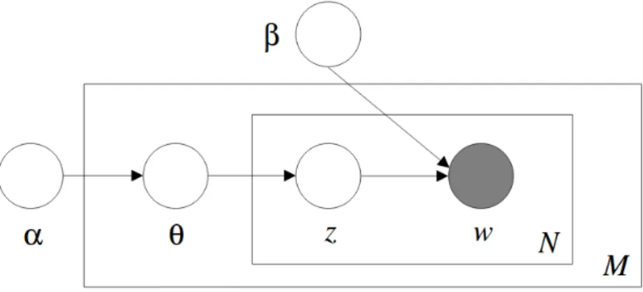
In 2003, D. Blei, Michelle Jordan and Andrew Ng proposed a model named Latent Dirichlet Allocation (LDA) in [14]. It is a generative statistical model for modeling documents. LDA assumes that a document is a bag of words, i.e.: the document “Hello my name is Haritz” is the same as “Haritz name Hello my is”. Furthermore, LDA assumes that a document is created as follows:
1. Pick N, the number of words.
2. Choose θ ∼ Dir(α1, ..., αk). θ is a topic mixture which lies in the k − 1
dimensional simplex. 3. For each of the N words:
(a) Choose a topic zn∼M ultinomial(θ).
(b) Choose a wordwnfromP(wn|zn), a multinomial probability conditioned
on the topic zn.
More formally, the joint probability distribution of a topic mixture θ, a set of N
topics z and a set of N words w is given by:
p(θ,z,w|α, β) =p(θ|α)
N Y n=1
p(zn|θ)p(wn|zn, β)
Integrating over θ and summing over z, we obtain the marginal distribution of a document: p(w|α, β) = Z p(θ|α) N Y n=1 X zn p(zn|θ)p(wn|zn, β) ! dθ
Finally, taking the product of the marginal probabilities of single documents, we obtain the probability of a corpus:
p(D|α, β) = M Y d=1 Z p(θd|α) Nd Y n=1 X zdn p(zdn|θd)p(wdn|zdn, β) ! dθd
The parameters α andβ are corpus-level parameters. They are sampled once in the process of generating a corpus. The variables θd are document-level variables
sam-pled once per document. Finally, the variables zdn and wdn are word-level variables
and are sampled once for each word in each document.
Figure 2.2: Graphical model representation of LDA
LDA does not assign names to the topics. The topics it provides are abstract so we have to assign labels to each topic in order to understand them better. Let’s see how a document is created according to LDA with an example. Let’s say we want a document with five words and two topics: food and animals. Each topic is composed of a map of (word, probability). The topics are the following:
• Topic 1: (broccoli, 0.3), (banana, 0.15), (breakfast, 0.1), (munching, 0.1), ... We will assign the label food.
• Topic 2: (chinchillas, 0.2), (cats, 0.2), (cute, 0.2), (hamster, 0.15), ... We will assign the label animals.
A possible document created using that data is: “Broccoli cute munching cats ba-nana”. As we can see, the document is not grammatically correct because documents are bags of words for LDA and nothing else. When we apply LDA to a document written by a person, it will assume that the document has been written as in the example, therefore, it will try to find the mixture of topics and their multinomial distributions which have generated it.
2.5.1
Inference
In order to use LDA, computing the posterior distribution of the hidden variables given a document is needed:
p(θ,z|w, α, β) = p(θ,z,w|α, β)
p(w|α, β)
Unfortunately, this distribution is intractable. Nevertheless, a wide variety of ap-proximate inference algorithms are available for LDA.
2.5.2
Variational Inference
A simple way to obtain a tractable family of lower bounds is to consider simple modifications of the original graphical model in which some of the edges and nodes are removed.
Figure 2.3: Graphical model representation of the variational distribution used to approximate the posterior in LDA
The distribution of this simplified graphical model is:
q(θ,z|γ, ϕ) = q(θ|γ)
N Y n=1
q(zn|ϕn)
where the Dirichlet parameter γ and the multinomial parameters ϕ1, ...ϕn are the
free variational parameters. To determine these parameters, it is needed to set up the following optimization problem:
(γ∗, ϕ∗) = arg min
(γ,ϕ)
D(q(θ,z|γ, ϕ) || p(θ,z|w, α, β))
Minimizing the Kullback-Leibler (KL) divergence between the variational distribu-tion and the true posterior p(θ,z|w, α, β) is possible to obtain the optimal values of the variational parameters. The minimization can be achieved via an iterative fixed-point method. Developing that formula, we obtain the following two formulas:
γi =αi+ N X n=1
ϕni
The expectation in the multinomial update can be computed as follows:
Eq[log(θi)|γ] = Ψ(γi)−Ψ( k X
j=1
γj)
All the calculations can be read in [14]. This yields to the following algorithm:
Algorithm 1 Variational Inference for LDA
1: ϕ0ni←1/k .for all i and n
2: γi ←αi +N/k . for all i 3: repeat 4: for n = 1 to N do 5: for i = 1 to k do 6: ϕtni+1 ←βiwnexp(Ψ(γ t i)) 7: normalize ϕtni+1 to sum 1 8: end for 9: γt+1 ←α+PN n=1ϕtn+1 10: end for 11: until convergence
From the pseudo code it is easy to see that each iteration of variational inference of LDA takes O(N k+N) operations.
2.6
Related models
2.6.1
Pachinko Allocation Model
Latent Dirichlet allocation (LDA) and other related topic models are very popular tools for summarization of texts. However, LDA does not capture correlations be-tween topics. Wei Li and Andrew McCallum introduced the the Pachinko Allocation Model (PAM) in [15]. It uses a directed acyclic graph (DAG) structure to represent topic correlations. Each leaf node is associated with a word and each non-leaf node corresponds to a topic. In figure 2.4 (c) and (d), it is possible to see the structure. For instance, given the topics: ”health”, ”cooking”, ”insurance” and ”drugs” the first topic occurs often with the second one and with the two remaining ones. Each of these topics would have a node and all of them would be at the same level. There
would be two additional nodes at a higher level. One would be the parent of cooking and health and the other one the parent of health, insurance and drugs.
LDA can be viewed as a special case of PAM: the DAG corresponding to LDA is a three-level hierarchy consisting of one root at the top, a set of topics in the middle and words at the bottom. The root is fully connected to all the topics, and each topic is fully connected to all the words. It is shown in 2.4 (b).
In PAM each topic ti is associated with a Dirichlet distribution gi(αi), where αi is
a vector with the same dimension as the number of children in ti . To generate a
document d, we follow the following process:
1. Sample θt(1d), θt(d2), ..., θt(sd) fromg1(α1), g2(α2), ..., gs(αs),where θt(di) is a
multino-mial distribution of topicti
2. For each word w in the document:
• Sample a topic path zw of length Lw
• Sample word w from θz(dw)(i−1)
Figure 2.4: Pachinko Allocation
2.6.2
Latent Semantic Indexing
Latent Semantic Indexing is a technique that projects queries and documents into a space with “latent” semantic dimensions. This space has fewer dimensions than the original space so it is a method for dimensionality reduction like PCA. Latent semantic indexing is the application of Singular Value Decomposition or SVD to a word-by-document matrix.
SVD takes a matrix A and represents it as ˆAin a lower dimensional space such that the “distance” between the two matrices measured by the 2-norm is minimized:
∆ =|A−Aˆ2|
LSI assumes the following:
• Concepts are represented as sets of words that usually appear together in documents. For example ”banana”, ”apple”, and ”strawberry” may usually appear in documents about fruits.
• Words are assumed to have only one meaning. Polysemy is a difficult problem for LSI so it uses this simplification.
2.6.3
Hierarchical LDA
This is a variant of LDA in which the goal is to obtain a hierarchy of topics given a collection of documents. General topics are at a high level while very specific topics are at lower levels. To generate a document, it samples a topic path from the hierarchy and then samples words from those topics. Therefore, a document can be about a mixture of Computer Science, Artificial Intelligence and Autonomous Robotics.
2.7
Data Mining
Data Mining is an interdisciplinary subfield of Computer Science that deals with the extraction of non-trivial, implicit, previously unknown and potentially useful patterns or knowledge from huge amount of data. It is also known as Knowledge Discovery in Databases (KDD) [16].
KDD has the following stages: 1. Data Selection
2. Data Cleaning and Preprocessing 3. Data Reduction and Transformation 4. Data Mining
5. Interpretation and Evaluation
2.7.1
Data Selection
It involves the search of datasets to use in the following steps. It is possible to use databases, plain-text documents, formatted documents, spreadsheets, etc.
2.7.2
Data Cleaning and Preprocessing
Data in the real world is dirty, i.e.: it is incomplete, noisy, inconsistent, etc. This affects to the machine learning algorithms to obtain patterns, so this step is needed to obtain a good data set. According to [16], it may take 60% of the total time used in the KDD process.
2.7.3
Data Reduction and Transformation
It includes the combination of data from different sources, resolving conflicts in units, removal of redundancy, aggregation, generalization and normalization of data.
2.7.4
Data Mining
It is the application of machine learning algorithms to the data obtained in the previous steps. The problems it can solve among others are:
• Classification
• Regression
• Clustering
• Association rules
2.7.5
Interpretation and Evaluation
It is the evaluation Interpretation and Evaluation by the domain experts of the patterns or new knowledge found. Visualization tools are usually needed.
Chapter 3
Proposal
In this chapter, the functionality of the libraries needed will be explained. First, we will show how the Twitter REST and Streaming APIs work. Then, we will explain how to preprocess the downloaded Tweets. After that, the Gensim’s implementation of Online LDA will be explained and the results will be interpreted using pyLDA, a visualization tool for LDA.
3.1
How to retrieve Tweets
Twitter offers an API to read and write Twitter data, create new Tweets, read user profiles and follower data, and more. The REST API identifies Twitter applications and users using OAuth and their responses are in JSON format.
3.1.1
How to gain access to the Twitter API?
At the apps page of Twitter, https://apps.twitter.com/ it is possible to create a new application. Since we do not have a web page, we can put: ”https://www.twitter.com” in the form when we are asked to enter our website. Then, we need to search the API Key and the API Secret. We will need them for accessing Twitter in our Python code.
Instead of using directly the Twitter API, Twython has been used. It is a wrapper for the Twitter API which allows us to get the responses from Twitter in Python objects instead of JSON.
Figure 3.1 shows the class diagram of the class Twython. As we can see, it is a simple class without any relationship like composition, aggregation or inheritance.
Figure 3.1: Class Diagram of the class Twython
Figure 3.2 shows the inheritance relationship in the exception classes defined by Twython. TwythonError is a general error class which inherits from exceptions.Exception. It also has three children classes for each of the possible errors that can happen using this library: TwythonAuthError, TwythonStreamError and TwythonRateLimitEr-ror. In addition, it has defined a warning, TwythonDepecrationWarning, which is a exceptions.DeprecationWarning. This last one is a exceptions.Warning which inher-its from exceptions.Exception. TwythonDepecrationWarning is used to warn about using a deprecated feature.
3.1.2
REST API
The REST API provides access to read and write data in Twitter. For example, it is possible to create new Tweets, read user profiles, etc.
This API has a limit of queries per time-window which is 15 minutes length. Depend-ing on the query, the number of possible queries is different [17]. A few commands are shown next:
The function get user timeline [18] retrieves tweets of a given user. This function can only return up to 3,200 of a user’s most recent Tweets. Its parameters, among others, are:
• screen name: The screen name of the user for whom to return results for.
• User id: The ID of the user for whom to return results for.
• count: Specifies the number of Tweets to try and retrieve, up to a maximum of 200 per distinct request.
• max id: Returns results with an ID less than (that is, older than) or equal to the specified ID.
• since id: Returns results with an ID greater than (that is, more recent than) the specified ID.
An example of this function is:
Example 3.1: get user timeline function
u s e r _ t i m e l i n e=t w i t t e r.g e t _ u s e r _ t i m e l i n e(s c r e e n _ n a m e=" M e r c e d e s A M G F 1 " , c o u n t= 1 0 ) # get a l i s t of d i c t i o n a r i e s . A T w e e t is i n s i d e a d i c t i o n a r y for t w e e t in u s e r _ t i m e l i n e: # p r i n t s T w e e t s and o t h e r i n f o r m a t i o n p r i n t t w e e t[’ t e x t ’] + " " + t w e e t[’ c r e a t e d _ a t ’] + " " + str( t w e e t[’ r e t w e e t _ c o u n t ’]) + " " + t w e e t[’ l a n g ’] + " " + t w e e t [’ i d _ s t r ’]
The function search [19] returns a collection of relevant Tweets matching a specified query. In addition to the parameters which get user timeline has, it has two new ones:
• q: The query
• result type: It is optional. It specifies what type of search results you would prefer to receive. It can have three possible values:
– recent: Returns only the most recent results in the response – popular: Returns only the most popular results in the response.
– mixed: Includes both popular and real time results in the response. Example 3.2: search function
t w e e t s _ s e a r c h e d = t w i t t e r.s e a r c h(q=’ C a n a d a ’, r e s u l t _ t y p e=’ r e c e n t ’, c o u n t= 1 0 ) for t w e e t in t w e e t s _ s e a r c h e d[’ s t a t u s e s ’]: p r i n t t w e e t[’ t e x t ’] + " " + t w e e t[’ c r e a t e d _ a t ’] + " " + str( t w e e t[’ r e t w e e t _ c o u n t ’]) + " " + t w e e t[’ l a n g ’] + " " + t w e e t [’ i d _ s t r ’]
The function get followers list [20] returns a collection of user objects for users fol-lowing the specified user. Among other parameters, it has:
• user id: The ID of the user for whom to return results for.
• screen name: The screen name of the user for whom to return results for.
• count: The number of users to return per page, up to a maximum of 200. Example 3.3: get followers list function
f o l l o w e r s = t w i t t e r.g e t _ f o l l o w e r s _ l i s t(s c r e e n _ n a m e = " @ J u s t i n T r u d e a u ", c o u n t= 1 0 )
for f o l l o w e r in f o l l o w e r s[" u s e r s "]:
p r i n t f o l l o w e r[’ s c r e e n _ n a m e ’] + " " + f o l l o w e r[’ n a m e ’] + " " +
f o l l o w e r[’ l o c a t i o n ’]
Now, the following question arises: ”How can I retrieve all followers of a user?” For example, Justin Trudeau, the Prime Minister of Canada, has more than 200 followers but the count parameter has an upper limit of 200. In order to do that, there is another parameter called cursor which lets us paginate the results. So the following code does the same as before:
Example 3.4: example of cursor parameter n e x t _ c u r s o r = -1 for i in x r a n g e(2) : f o l l o w e r s = t w i t t e r.g e t _ f o l l o w e r s _ l i s t(s c r e e n _ n a m e = " @ J u s t i n T r u d e a u ", c o u n t=5 , c u r s o r=n e x t _ c u r s o r) for f o l l o w e r in f o l l o w e r s[" u s e r s "]: p r i n t f o l l o w e r[’ s c r e e n _ n a m e ’] + " " + f o l l o w e r[’ n a m e ’] + " " + f o l l o w e r[’ l o c a t i o n ’] n e x t _ c u r s o r = f o l l o w e r s[’ n e x t _ c u r s o r ’] # W A T C H OUT H E R E ; it is f o l l o w e r s , not f o l l o w e r
This code retrieves 2 pages of the followers of Justin Trudeau and there are 5 follow-ers on each page. We could add more followfollow-ers to each page modifying the parameter count.
Thanks to Twython, there will be a better way to do it. Twython has implemented the function cursor to manage the cursor for us, but right now has a bug and it is in the process of being fixed [21].
3.1.3
Streaming API
It allows access to Twitter’s global stream of Tweet data [22]. It should be used when real-time data from Twitter is needed. This API does not have a rate limit as the REST API. In order to use this API we need to create the following class:
Example 3.5: Class MyStreamer
f r o m t w y t h o n i m p o r t T w y t h o n S t r e a m e r c l a s s M y S t r e a m e r(T w y t h o n S t r e a m e r) : def o n _ s u c c e s s(self, d a t a) : if ’ t e x t ’ in d a t a: p r i n t d a t a[’ t e x t ’].e n c o d e(’ utf -8 ’) def o n _ e r r o r(self, s t a t u s _ c o d e, d a t a) : p r i n t s t a t u s _ c o d e, d a t a # W a n t to s t o p t r y i n g to get d a t a b e c a u s e of the e r r o r ? # U n c o m m e n t the n e x t l i n e ! # s e l f . d i s c o n n e c t ()
Which can be instantiated it as follows:
Example 3.6: Get tweets in real time s t r e a m = M y S t r e a m e r(APP_KEY, A P P _ S E C R E T,
O A U T H _ T O K E N, O A U T H _ T O K E N _ S E C R E T)
S e a r c h T e r m = ’ T r u d e a u ’ # If s p a c e s are i n c l u d e d , t h e y are ’ OR ’ , ie f i n d s t w e e t s w i t h any one of the words , not the w h o l e s t r i n g .
T w e e t e r = ’ 2 5 0 7 3 8 7 7 ’ # T h i s is D o n a l d Trump , f i n d s t w e e t s f r o m him or m e n t i o n i n g him s t r e a m.s t a t u s e s.f i l t e r(t r a c k=S e a r c h T e r m) # Or # s t r e a m . s t a t u s e s . f i l t e r ( f o l l o w = T w e e t e r )
3.2
Data Retrieval
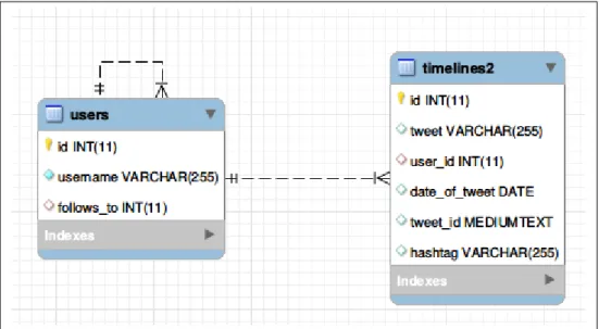
LDA needs documents as input, so we have downloaded Tweets and grouped them in documents. First, Tweets have been stored in a database. This allows us to create different documents with the same Tweets. The database has the following schema:
Figure 3.3: Schema of the database
The table users have a one-to-many self-relationship which models that one user has many followers. In addition, it has a one-to-many relationship with the table timelines2. Each row of this table represents a Tweet. It has an id column which is filled automatically by MySQL when it is stored and a tweet id column in which it is stored the id that Twitter gives to that Tweet.
Before storing the Tweets, a small preprocessing has been done. The hashtags have been retrieved and stored, the words “RT”, which stands for retweet, have been removed; idem with the usernames when somebody was quoted, all non-ASCII characters like “˜n” or “´ı” and the hashtags.
In order to create the files, i.e.: the documents, we have differentiated between followed users (famous people in our case) and followers. In the first case, Tweets have been grouped by hashtag, so a document is a set of Tweets with the same hashtag. All Tweets without hashtag have been grouped in the same document and then this document has been divided into chunks of 10 KiB. In the case of followers of a user, a document has been created per user. This last approach has also been followed in [8].
The following code shows how to create the documents from The New York Times’ Tweets. It is trivial to modify it in order to create all the documents of all the users in the database.
Example 3.7: Create documents of The New York Times
i m p o r t M y S Q L d b
c o n n = M y S Q L d b.c o n n e c t(h o s t= " l o c a l h o s t ",
p a s s w d=" h a r i t z ", db=" N L P _ T F G ") c u r s o r = c o n n.c u r s o r() c o n c a t = " SET g r o u p _ c o n c a t _ m a x _ l e n = 1 8 4 4 6 7 4 4 0 7 3 7 0 9 5 5 1 6 1 5 ; " c u r s o r.e x e c u t e(c o n c a t) s e l e c t T w e e t s = """ S E L E C T G R O U P _ C O N C A T ( t w e e t S E P A R A T O R ’ ’) , h a s h t a g F R O M N L P _ T F G . t i m e l i n e s 2 t W H E R E t . u s e r _ i d = 3 1 2 2 and h a s h t a g != ’ ’ G R O U P BY hashtag , u s e r _ i d ; """ c u r s o r = c o n n.c u r s o r() c u r s o r.e x e c u t e(s e l e c t T w e e t s) # F e t c h all the r o w s in a l i s t of l i s t s . r e s u l t s = c u r s o r.f e t c h a l l() cnt = 1
for t w e e t in r e s u l t s: # for e a c h doc
n a m e O f D o c = t w e e t[1] doc = o p e n(’ / h o m e / h a r i t z / TFG / n y t i m e s _ h a s h t a g s 2 / ’ + n a m e O f D o c+ ’ . txt ’, ’ a ’) # a p p e n d i n g doc.w r i t e(t w e e t[ 0 ] ) doc.w r i t e(" ") doc.c l o s e() # t w e e t s w i t h o u t h a s h t a g s e l e c t T w e e t s W i t h o u t H a s h t a g = """ S E L E C T t w e e t F R O M N L P _ T F G . t i m e l i n e s 2 t W H E R E t . u s e r _ i d = 3 1 2 2 and h a s h t a g = ’ ’; """ n o H a s h t a g C u r s o r = c o n n.c u r s o r() n o H a s h t a g C u r s o r.e x e c u t e(s e l e c t T w e e t s W i t h o u t H a s h t a g) # F e t c h all the r o w s in a l i s t of l i s t s . r e s u l t s = n o H a s h t a g C u r s o r.f e t c h a l l() cnt = 1
for t w e e t in r e s u l t s: # for e a c h doc
n a m e O f D o c = str(cnt) cnt += 1 doc = o p e n(’ / h o m e / h a r i t z / TFG / n y t i m e s _ h a s h t a g s 2 / ’ + n a m e O f D o c + ’ . txt ’, ’ a ’) # a p p e n d i n g doc.w r i t e(t w e e t[ 0 ] ) doc.w r i t e(" ") doc.c l o s e()
3.3
Modeling users’ timelines with LDA
Gensim’s [23] LDA algorithm implements Online LDA [24] in Python. It needs three parameters:
• Corpus: A vector of (word id, number of occurrences)
• Number of topics
• Dictionary: a mapping between words id and words Example 3.8: Example LDAModel
g e n s i m.m o d e l s.l d a m o d e l.L d a M o d e l(corpus, n u m _ t o p i c s, d i c t i o n a r y)
Figure 3.4 shows the class diagram of the class LDAModel. It is worth noting the composition between LDAModel and LDAState. An LDAModel has one LDAState.
3.3.1
How to create a corpus?
First, a list of documents is needed. It is possible to obtain it with the following code:
Example 3.9: read data
def r e a d _ d a t a(p a t h) : d o c s = [] for f i l e _ n a m e in os.l i s t d i r(p a t h) : f i l e = o p e n(p a t h + f i l e _ n a m e) d o c s.a p p e n d(u n i c o d e(f i l e.r e a d() , e r r o r s=’ r e p l a c e ’) ) r e t u r n d o c s Data Cleaning
Data cleaning is the most important step in natural language processing. In the case of Twitter, this task is even more difficult due to the length of the Tweets and the topic diversity. First of all, all words have been converted to lowercase. Then, each document has been split into words. After that, all numbers have been removed, but words with numbers have been kept. Next, words with three characters or less have been removed because short words like ”to”, ”I”, ”me”, etc. do not help the algorithm. Next, stopwords have been removed using the nltk stopwords list. After that, words have been lemmatized. It is a transformation of the word to convert it into the word’s lemma, or dictionary form. For instance: ”are” is transformed into ”be” and ”cats” into ”cat”. Furthermore, bigrams have also been taken into account. There are words like New York or San Francisco which are
Figure 3.4: Class Diagram of LDAModel
always together. Using bigrams we can detect them and treat them as only one. In the code below, we find bigrams and then, add them to the original data, because we would like to keep the words ”machine” and ”learning” as well as the bigram ”machine learning”. Computing n-grams of a large dataset can be computationally and memory expensive.
This is the code that used for preprocessing the data. Example 3.10: preprocessing
def p r e p r o c e s s i n g(d o c s) :
# S p l i t the d o c u m e n t s i n t o t o k e n s .
t o k e n i z e r = R e g e x p T o k e n i z e r(r ’ \ w + ’)
s t o p s = set(s t o p w o r d s.w o r d s(’ e n g l i s h ’) ) # n l t k s t o p w o r d s l i s t
for idx in r a n g e(len(d o c s) ) :
d o c s[idx] = d o c s[idx].l o w e r() # C o n v e r t to l o w e r c a s e .
d o c s[idx] = t o k e n i z e r.t o k e n i z e(d o c s[idx]) # S p l i t i n t o w o r d s .
# R e m o v e numbers , but not w o r d s t h a t c o n t a i n n u m b e r s .
d o c s = [[t o k e n for t o k e n in doc if not t o k e n.i s n u m e r i c() ] for
doc in d o c s]
# R e m o v e w o r d s t h a t <= t h r e e c h a r a c t e r .
d o c s = [[t o k e n for t o k e n in doc if len(t o k e n) > 3] for doc in
d o c s]
d o c s = [[t o k e n for t o k e n in doc if t o k e n not in s t o p s] for doc
in d o c s]
# L e m m a t i z e all w o r d s in d o c u m e n t s .
l e m m a t i z e r = W o r d N e t L e m m a t i z e r()
d o c s = [[l e m m a t i z e r.l e m m a t i z e(t o k e n) for t o k e n in doc] for doc
in d o c s]
# Add b i g r a m s to d o c s ( o n l y o n e s t h a t a p p e a r 20 t i m e s or m o r e ) .
b i g r a m = g e n s i m.m o d e l s.P h r a s e s(docs, m i n _ c o u n t= 2 0 )
for idx in r a n g e(len(d o c s) ) :
for t o k e n in b i g r a m[d o c s[idx]]:
if ’ _ ’ in t o k e n:
# T o k e n is a bigram , add to d o c u m e n t .
d o c s[idx].a p p e n d(t o k e n)
r e t u r n d o c s
Dictionary and corpus
Once we have the data preprocessed, creating the dictionary and the corpus is straightforward thanks to Gensim.
Example 3.11: get dictionary
def g e t _ d i c t i o n a r y(t e x t s) : # t u r n our t o k e n i z e d d o c u m e n t s i n t o a id < - > t e r m d i c t i o n a r y d i c t i o n a r y = c o r p o r a.D i c t i o n a r y(t e x t s) # d i c t i o n a r y . f i l t e r _ e x t r e m e s ( n o _ b e l o w =20 , n o _ a b o v e = 0 . 5 ) d i c t i o n a r y.f i l t e r _ n _ m o s t _ f r e q u e n t(5) r e t u r n d i c t i o n a r y
Example 3.12: get corpus
def g e t _ c o r p u s(d i c t i o n a r y, t e x t s) :
# c o n v e r t t o k e n i z e d d o c u m e n t s i n t o a d o c u m e n t - t e r m m a t r i x
u s e r s _ c o r p o r a = [d i c t i o n a r y.d o c 2 b o w(t e x t) for t e x t in t e x t s]
r e t u r n u s e r s _ c o r p o r a
Figure 3.5 shows the class Dictionary, which is a subclass of Mapping. This last class is a subclass of Container, Iterable and Sized. This is possible because Python sup-ports multiple inheritance in contrast to Java. The module abcoll defines abstract base classes for collections.
Figure 3.5: Class Diagram of Dictionary
3.3.2
LDA Model
The function LdaModel has three mandatory parameters as we stated before: the corpus, the number of topics and the dictionary. So creating an LDA model is easy
since we have already created the auxiliary functions explained before. Example 3.13: LdaModel d o c s = r e a d _ d a t a(p a t h) t e x t s = p r e p r o c e s s i n g(d o c s) d i c t i o n a r y = g e t _ d i c t i o n a r y(t e x t s) u s e r s _ c o r p o r a = g e t _ c o r p u s(d i c t i o n a r y, t e x t s) g e n s i m.m o d e l s.l d a m o d e l.L d a M o d e l(u s e r s _ c o r p o r a, n u m _ t o p i c s= n u m _ t o p i c s, i d 2 w o r d = d i c t i o n a r y)
In addition to the three main parameters mentioned before, LdaModel has several optional parameters. In this thesis, we have used the following:
• alpha: hyperparameter that affects sparsity of the document-topic distribu-tion. The lower it is, the lower the number of topics per documents.
• eta: hyperparameter that affects sparsity of the topic-word distribution. The lower it is, the lower the number of words per topic.
• passes: puts a limit on how many times LDA will execute the E-Step for each document, meaning that some documents may not converge in time.
• iterations: allows LDA to see the corpus multiple times. It is very handy for small corpora.
3.3.3
Data Visualization
Once models are created, we need to interpret them. It is possible to obtain the distributions of the models executing the following code:
Example 3.14: Retrieving topic distributions
for i in x r a n g e(n u m b e r _ o f _ t o p i c s) : # for e a c h t o p i c
p r i n t ’ T o p i c ’ + str(i)
for tup in s m a l l _ l d a m o d e l.g e t _ t o p i c _ t e r m s(i, t o p n=len(
d i c t i o n a r y) ) :
p r i n t d i c t i o n a r y.get(tup[ 0 ] ) + " " + str(tup[ 1 ] ) # ( word , p r o b a b i l i t y )
Nevertheless, it is difficult to obtain a quick global idea of the topics. Data Visu-alization has a huge importance in the interpretation step of data mining. That is why there are so many data visualization libraries. LDAvis [25] is a web-based interactive visualization of LDA topics built using R and D3 for Python and R. The objective of LDAvis is to answer the following questions:
2. How prevalent is each topic?
3. How do the topics relate to each other? LDAvis is composed of two parts:
• Left panel: Gives a global view of the topic model. It answers questions 2 and 3. The area of each circle means the topic’s overall prevalence and the location of each circle is determined by computing the distance between topics.
• Right panel: Answers question 1. It is composed of horizontal bars. Each bar represents a term for the selected topic. The bars in blue represents the overall term frequency while the red ones the estimated term frequency within the selected topic. In addition, there is a λ parameter which is a weight for the relevance of a term to a topic.
LDAvis ranks the terms within a topic using its relevance.
relevance=r(w, k|λ) = λlog(φkw) + (1−λ)log(
φkw
pw
) where
log(φkw) = P(word=w|topic=k)
Figure 3.6: Example of a graphical model
The lambda parameter allows us to modify how we want to compute the relevance. If λ= 1, then:
In this case, the shown words would be relative to the overall corpus but not neces-sarily to the topic. On the other hand, if Ifλ = 0, then:
relevance=r(w, k|λ= 0) =log(φkw
pw
)
and this implies that words which appear a lot in the corpus do not have a high relevance while words that appear a few times times in the corpus would have a high relevance.
3.3.4
Use of Gensim’s LDA
First, LDA has been executed on a small corpus created with articles from Wikipedia. This corpus is composed of three documents:
• One about Fernando Alonso, a Spanish F1 pilot.
• One about Barack Obama, President of the United States of America.
• One about Kurt G¨odel, one of the most important logicians in the history. After the execution of the following code:
Example 3.15: LdaModel
(model, corpus, t e x t s) = g e t _ L D A _ m o d e l(p a t h _ t o _ t e s t _ d o c u m e n t s 1, 3)
l d a _ D a t a = p y L D A v i s.g e n s i m.p r e p a r e(model, corpus, g e t _ d i c t i o n a r y(
t e x t s) )
p y L D A v i s.d i s p l a y(l d a _ D a t a)
A model with three topics have been obtained. Using LDAvis to interpret the topics, it is possible to clearly identify three separated topics: the first one about Fernando Alonso, the second one about Barack Obama and the last one about Kurt G¨odel.
Figure 3.7: Topic 1: Alonso
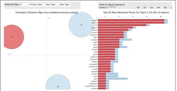
Figure 3.9: Topic 3:Kurt G¨odel
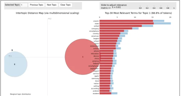
Another small test has been done. In this case, the following documents have been used:
• An article in Wikipedia about Xiaomi Inc., a Chinese mobile phone manufac-turer.
• An article in Wikipedia about the United States of America.
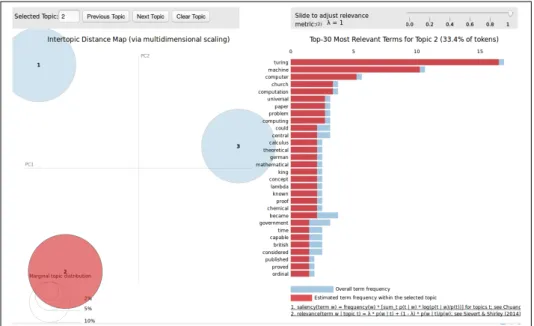
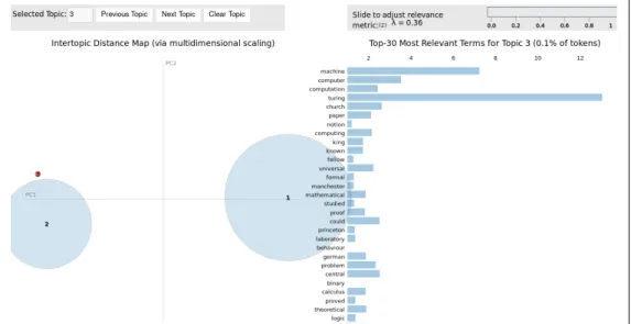
• An article about Alan Turing, the father of the Theoretical Computer Science and Artificial Intelligence.
Figure 3.11: Topic 2: Turing
Figure 3.12: Topic 3: Xiaomi
The creation of a model is a random process, so in each execution of the algorithm, it gives different results. Figure 3.13, 3.14 and 3.15 represent a bad model. The dataset is exactly the same one as before: one document about Xiaomi, another one about Turing and the last one about the USA.
Figure 3.13: Bad model - Topic 1. It is a mixture of Xiaomi and United States.
Figure 3.14: Bad model - Topic 2. It is about Turing but it also has the word Xiaomi.
Figure 3.15: Bad model - Topic 3. It is a really small topic which does not make any sense.
Chapter 4
Results
In this chapter, the focus will be in the generation of LDA models, its analysis and the comparison of the topics obtained from a user and their followers. An analysis of the results including if the results given are valid and accurate will be provided. All the data has been retrieved between April 28, 2017 and May 3, 2017 taking into account that Twitter only allows to download up to 3,200 of a user’s most recent Tweets.
4.1
Barack Obama’s Topics
LDA has been able to recognize several topics among the Tweets of Barack Obama. The second topic, shown in figure 4.1, is clearly about climate change. It contains words like ”climate”, ”climate change”, ”clean”, ”energy”, ”fight”, ”carbon”, ”pol-lution”, etc. We can see that most of the words of this topic are only relevant in it because the red bar is almost as big as the blue one.
Figure 4.1: Topic 2: Climate Change
The third topic, shown in figure 4.2, is about the Supreme Court nomination Merrick Garland. Barack Obama nominated him for the Supreme Court but the Republican senate was against it so the judge Merrick Garland could not have a sit at the Supreme Court. The words that allow us to label this topic this way are: ”senate”, ”judge”, ”garland”, ”supreme court”, ”nominee”, ”obstruction”, etc. We can see again that most of the words of this topic are only relevant in it for the same reason as before.
Figure 4.2: Topic 3: Merrick Garland Supreme Court nomination
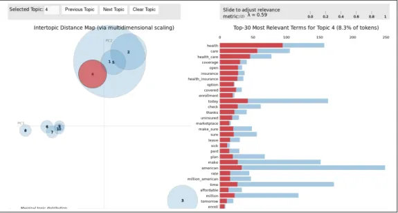
The fourth topic, shown in figure 4.3, seems to be about the Patient Protection and Affordable Care Act commonly known as Obamacare. The words of this topic are about health and insurance for example: ”healh care”, ”uninsured”, ”sick”, ”coverage”, ”affordable”, ”million american”, etc. In this topic, we can see that
there are many words which are relevant in other topics because the red bars are not as big as the blue ones.
Figure 4.3: Topic 4: Health Care
With the fifth topic, shown in figure 4.4, labeling starts to be more difficult. Words like ”immigration”, ”system”, ”immigrant”, ”congress” and ”violence” may indicate that this topic is about immigration. It is worthwhile noting that the word violence appears but LDA does not tell us its meaning. It could have been used to indicate that immigrants are not violent or the contrary. It is also important to note that the relevance of this topic in the corpus is really small. We can see this because the bars are usually very small.
Figure 4.4: Topic 5: Immigration
It contains words like ”minimum”, ”wage”, ”raising”, ”earning”, ”poverty” and ”private sector” so it can be labeled as ”Salaries”. This topic is not too relevant in the corpus since the size of the cluster is small in comparison with other clusters.
Figure 4.5: Topic 6: Salaries
Once the topics are analyzed it is possible to state that Barack Obama writes on Twitter about his politics.
4.2
Barack Obama’s Followers’ Topics
Unfortunately, Standard LDA has not been able to obtain any topics with some sense for humans. All of them are a mixture of unrelated words or without a useful meaning. For example, in topic 7, shown in figure 4.6, there are words like ”good”, ”time”, ”people”, ”life”, ”look”, ”think”, ”need”, ”year”, ”right”, ”know”, etc. Those words are not useful to label this topic. Most of the topics are similar to this one.
Figure 4.6: Topic 7: It’s not possible to label it.
4.3
NASA’s Topics
All the LDA topics generated share words like mission, space, etc. Nevertheless, LDA has been able to generate some topics which can be interpreted by humans. The first topic, shown in figure 4.7, contains words like ”space”, ”launch”, ”spacecraft”, ”crew”, ”mission”, ”moon”, ”cargo” and ”cygnus” so it is possible to conclude that it is about the Cygnus Spacecraft launch. We can see that the blue bars are bigger than the red ones. This means that the words of this topic are relevant in other topics. As stated before, words like space and earth appears in many topics.
Figure 4.7: Topic 1: Cygnus Spacecraft launch
The fifth topic, shown in figure 4.8 contains words like ”spacewalk”, ”astronaut”, ”earth”, ”look”, ”view” and ”outside”, so we can label it as ”Spacewalk”. In this
case, the word ”spacewalk” is only relevant in this topic because the red bar is almost as big as the blue one. ”outside” is not a word that appears too much in the corpus but it is quite relevant in this topic.
Figure 4.8: Topic 5: Spacewalk
The sixth topic, shown in figure 4.9, contains words like ”launch”, ”mission”, ”cygnss”, ”hurricane”, ”satellite”, ”weather” and ”forecasting” so it is easy to label it ”CYGNSS”. It is about a system sponsored by NASA to forecast hurricanes. As expected, the word ”cygnss” only appears in this topic since the red bar is as big as the blue one. The other words like ”launch”, ”mission” and ”satellite” describes this topic. This means that LDA has been able to recognize this topic correctly.
Figure 4.9: Topic 6: CYGNSS hurricane forecasting
The last topic that has been labeled is the eight one, shown in figure 4.10. It contains words like ”cargo”, ”dragon”, ”vehicle”, ”spacecraft”, ”supply”, ”carrying” and ”station” so it has been labeled as ”Dragon Cargo Vehicle”. In this case, LDA is able to identify correctly again the topic because words like ”dragon cargo” and
”dragon” are only relevant in this topic. We can see this because their red bars are almost as big as their blue ones. Words like ”vehicle”, ”supply” and ”spacecraft” helps to understand this topic but also other topics, that is why they are also relevant in others.
Figure 4.10: Topic 8: Dragon cargo vehicle
After the analysis of all its topics, it is easy to see that as expected, NASA writes on Twitter about the space and its missions.
4.4
NASA’s Followers’ Topics
After executing LDA in the corpus, four well-defined topics have been found. The first topic, shown in figure 4.11, has been labeled: ”Politics” because it includes words like ”Trump”, ”Obama”, ”President”, ”democrat”, ”liberal” and ”Presi-dent Trump”. All these words are only relevant in this topic. This means that LDA has been able to define it well.
Figure 4.11: Topic 1: Politics
The third topic, shown in 4.12, is clearly about students since it contains words like ”student”, ”learning”, ”teacher”, ”school”, ”kid”, ”classroom”, ”educator”, etc. All those words are only relevant in this topic which means that in this case, LDA has been able again to define the topic well.
Figure 4.12: Topic 3: Students
The following well-defined topic is the eighth one, shown in figure 4.13. This topic is also easy to label since it contains words like ”social”, ”medium”, ”business”, ”marketing”, ”facebook”, ”strategy”, ”business social”, ”strategy” and ”brand” so it has been named: ”Marketing in Social Media”. Most of those words are mostly relevant only in this topics. Other words like ”Facebook” are relevant in other topics too as expected since it is a word used in many contexts, not only in marketing.
Figure 4.13: Topic 8: Marketing in Social Media
The last labeled topic is the ninth one, shown in figure 4.14. It has been called ”Music” since it has words like ”bossa”, ”Ernesto Nazareth”, ”Alatamiro Carrilho”, ”bossa nova”, ”Leny Andrage” and ”lista reprodu”. As we can see, most of the words only belongs to this topic. This means that this topic so specific that any of its words cannot be in used in any other topic.
Figure 4.14: Topic 9: Music
After this analysis, it is easy to see that NASA’s topics are not related to its followers since any of them wrote about the space or any space mission.
4.5
Lewis Hamilton’s Topics
Among the topics LDA has generated, a few topics can be interpreted by humans. The first one, figure 4.15, is about feeling grateful. It contains words like: ”thanks”, ”great”, ”love”, ”followed”, ”friend”, ”well” and ”happy birthday”. Probably he writes about this topic when he wins races or the F1 championship. As we can see, most of the words are not only relevant in this topic which means that this topic is not too specific, i.e.: its words can be used in other contexts or topics.
Figure 4.15: Topic 1: Feeling grateful.
The remaining topics are very noisy although it is possible to identify that the fourth, fifth and eight topics are about Grand Prix (GP). The fourth topic contains words like: ”Austrian GP”, ”Russian GP”, ”Abu Dhabi GP”, ”Brazilian GP”, ”Spanish GP”, ”Sochi” (the Russian city where the Russian GP takes place), ”Jerez (a Spanish city where sometimes there are F1 tests) and ”Yas Marina” (the name of the circuit of Abu Dhabi).
The other topics are difficult to label because although most of the words are related to Formula 1, they are a mixture of words which are not related to each other.
Figure 4.16: Topic 4: Grand Prix. Common words are: Austrian GP, Russian GP, Abu Dhabi GP, Brazilian GP, Spanish GP, Sochi (the Russian city where the Russian GP takes place), Jerez (the Spanish city where the Spanish GP takes place) and Yas Marina (the name of the circuit of Abu Dhabi).
Figure 4.17: Topic 5: Grand Prix. Common words are: Hungarian GP, British GP, Japanese GP, Malaysian GP, European GP, Chinese GP, Silverstone (the circuit of the UK), Suzuka (the Japanese circuit), Hungaroring (the Hungarian circiut) and Hammertime (a word which Hamilton uses a lot to refer his piloting style).
Figure 4.18: Topic 8: Grand Prix. Common words are: Barhain GP, Mexico GP, winter training, Singapore (there is a GP there) and F1isback.
In conclusion, Hamilton writes about F1 as expected.
4.6
Hamilton’s Followers’ Topics
A total of five topics has been identified. The first topic, figure 4.19, is about flights. It has words like: ”airport”, ”service”, ”international airport”, ”airline”, ”flight” and cities or countries like ”Bali” (a very touristic place), ”San Francisco”, ”Korea”, ”Melbourne”, ”York” and ”Australia”. This topic can be considered well defined and specific because most of its words are only relevant in this topic.
The following identified topic is the fourth one, figure 4.20. This one is about the Manchester United as it contains words like ”Manchester United”, ”Mourinho”, ”Gaal”, ”Zlatan”, ”Schweinteiger”, ”Pogba”, etc. In this case, LDA is able again to capture the structure of this topic successfully. Most of the words are only relevant in this topic and since all the words are related to each other we can state that the topic has been well identified.
Figure 4.20: Topic 4: Manchester United
The fifth topic (figure 4.21) seems to be about Kodak. It is composed of words like: ”Kodak”, ”Print”, ”nexpress” (it is a Kodak’s platform), ”digital”, ”inkjet”, ”printer” and more Kodak’s platforms. In this case, LDA is able again to capture the structure of this topic successfully. Most of the words are only relevant in this topic and all of them are related to each other so we can declare that this topic has been well defined.
Figure 4.21: Topic 5: Kodak
The next topic (figure 4.22) is trivial to associate it to Twitter since it is made of words like ”retweeted”, ”follower”, ”unfollowers”, ”gained”, ”unfollowed” and ”tweet stats”. The word ”follower” is relevant in this topic and others since its blue bar is much bigger than the red one. The remaining words are only relevant in this topic.
Figure 4.22: Topic 6: Twitter
Finally, the last well-defined topic is the eighth one (figure 4.23) which is about an Indian movie called ”Shivaay”. Almost all the compound words contains the word ”Shivaay”, for example: ”sunday shivaay”, ”teamshivvay”, ”shivaay shoot”, etc. It also contains words like ”bollywood” and ”premiere”. In this topic, only the words ”action”, ”sunday” and ”shoot” are relevant in other topics.
Figure 4.23: Topic 8: Shivay, an Indian movie
Again, the topics of the followers are not similar to the topics of the followed person.
4.7
New York Times’s Topics
In this case, LDA has not been able to obtain good topics. There is only one topic which can be given a label, war, but it is still not well defined. This topic is the number eight (figure 4.24). It contains words like ”Syria”, ”strike” and ”army”.
Figure 4.25: Topic 3: Contains words like ”Korea”, ”Jon Ossoof”, ”Church”, ”Mi-lano” and ”cursed”. The topic is not well defined because its word are not related to each other so we cannot assign it a label.
4.8
New York Times’ Followers’ Topics
Among the topics LDA has generated, only two have been well defined. The first one (figure 4.26) has been labeled as ”Politics” since it contains words like ”governor”, ”Clinton”, ”vote”, ”Obama”, ”Trump”, ”State” and ”conservative”.
Figure 4.26: Topic 2: Politics.
The following topic (figure 4.27) has been labeled as ”immigrants” since it is com-posed of words like ”immigrant”, ”undocumented”, ”Turkish”, ”Kurdish”, ”pro-tection”, ”border” and ”Trump”. Except this last word, the other words are only relevant in this topic, so we can affirm that this topic is well defined.