Analytics for directed contact networks

R E S E A R C H

Open Access

Analytics for directed contact networks

George Cybenko

and Steve Huntsman

*Correspondence:

steve.huntsman@baesystems.com 2_{BAE Systems FAST Labs, 4301} North Fairfax Drive, Arlington, VA 22203, VA, USA

Full list of author information is available at the end of the article

Abstract

Directed contact networks(DCNs) are temporal networks that are useful for analyzing and modeling phenomena in transportation, communications, epidemiology and social networking. Specific sequences of contacts can underlie higher-level behaviors such asflowsthat aggregate contacts based on some notion of semantic and temporal proximity. We describe a simple inhomogeneous Markov model to infer flows and taint bounds associated with such higher-level behaviors, and also discuss how to

aggregate contacts within DCNs and/or dynamically cluster their vertices. We provide examples of these constructions in the contexts of information transfers within

computer and air transportation networks, thereby indicating how they can be used for data reduction and anomaly detection.

Introduction

Directed contact networks (DCNs) are temporal networks in which edges are directed

(Holme2015; Masuda and Lambiotte2016). Loosely speaking, temporal networks have

time attributes associated with edges while directed contact networks have both time and direction attributes associated with edges. DCNs are a natural temporal generalization of digraphs, and we can think about them informally as collections of time-stamped and directed contacts between and among the entities represented by the nodes. A simple example of a directed contact network is a collection of call data records in which each record includes information about who placed the call, who received the call and the time of the call (Bianchi et al.2016).

In this paper, we address the problem of how directed contacts can be aggregated and coarsened for purposes such as anomaly detection. To accomplish this, we construct a natural inhomogeneous (that is, time varying) Markov model (Huntsman2018a) for prob-abilistic modeling of potentialflowsthat aggregate contacts based on a simple notion of spatiotemporal proximity. This model involves a single parameter, which in practice we set automatically with an intuitive heuristic. Through analytical and practical examples, we illustrate the behavior of this Markov model. We emphasize that this Markov model is not statistical in the sense that it involves no learning, fitting, optimization or other estimation procedure. Instead, it starts from a small number of symmetry and invari-ance requirements thatanymodel with its goals ought to obey. This follows a tradition in physics by exhibiting a general mathematical structure that is consistent with the required symmetries. Because of this generality, the model applies to a wide range of problems that can be modeled with directed contacts, including call data record analysis, network traffic analysis and disease surveillance.

We also introduce the concept of a “taint bound” that quantifies the impact of weighted contacts: for example, how much of a given information transfer can possibly propagate through the network. Using publicly available data on flight timetables, we demonstrate by analogy how such taint bounds can constrain data exfiltration within a computer system and network. Finally, we also discuss two ways of aggregating and coarsening networks of directed contacts through renormalization and clustering.

It is useful to note that a contact of any type, information or not, involves asource s, a target t, and atimeτassociated with the contact. For simplicity, we assume contacts occur at a given instant in time with the resulting notion of a directed contact as an ordered triple(s,t,τ). This still enables considerable generality: for instance, a transfer fromsto tover the time interval [τ0,τ1] can be represented by two contacts involving a surrogate

third node as(s,∗,τ0)and(∗,t,τ1)where∗is the surrogate placeholder for(s,t, [τ0,τ1]).1

The paper is structured as follows: “Directed contact networks and temporal

digraphs” section introduces directed contact networks and temporal digraphs; “Markov chain models for DCNs” section discusses our Markov model, and “Data reduction and anomaly detection” section discusses its performance in data reduction and anomaly detection. We then turn to taint bounds in “Taint bounds” section before discussing renormalization and clustering in directed contact networks in “Renormalization” section and “Clustering” section, respectively. “Remarks” section concludes the paper.

Directed contact networks and temporal digraphs

A particularly useful family oftemporal networksaredirected contact networks (DCNs) (Holme2015; Masuda and Lambiotte2016). DCNs are a natural temporal generalization of digraphs, and we can think about them informally as collections of contacts as intro-duced in “Introduction” section. However, to avoid certain degenerate cases, we provide a slightly more formal and restrictive notion here.

A DCN with verticesV =[n] := {1,. . .,n}is a finite nonempty setC, where eachcontact c ∈ C corresponds to a unique triple(s(c),t(c),τ(c)) ∈[n]×[n]×Rwiths(c) = t(c). As a matter of convenience, we identify contacts with their corresponding triples in this manner.

Next, define thetemporal fiber at v, C@v, to be the set of times at which vertexvis involved in a contact as either source or destination, together with the times plus and minus infinity. More formally,

C@v:= {±∞} ∪ {τ(c):c∈C∧(s(c)=v∨t(c)=v)} =:{τ_j@v}_j|C₌@₀v|−1. (1)

Thetemporal digraphofC(for an example, see Fig.1) is defined as the digraphT(C) with respective vertex and arc sets

V(T(C)) := {(v,±∞):v∈V}

∪{(v,τ(c)):[(v,c)∈V×C]∧[s(c)=v∨t(c)=v]} (2) A(T(C)) := {((s(c),τ(c)),(t(c),τ(c))):c∈C}

∪{((v,τ_j@₋v₁),(v,τ_j@v)):v∈V,j∈[|C@v| −1]}. (3)

1_{By analogy, consider a flight departing fromsatτ}

0and arriving attatτ1. Here the contact(s,∗,τ0)corresponds to

embarking, while the contact(∗,t,τ1)corresponds to debarking. We can think of∗as the physical plane on which the

passengers flew. Alternative representations involving additional contacts of the form(s,∗,τ∗)withτ0≤τ∗< τ1might

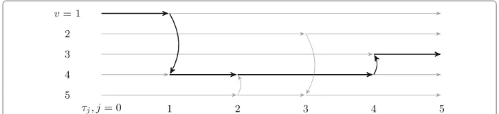
Fig. 1Temporal digraph of the DCN_C:= {(1, 4,τ1),(5, 4,τ2),(2, 5,τ3),(4, 3,τ4)}withτ1< τ2< τ3< τ4. We indicate a temporally coherent path from_C-vertices 1 to 3 with bold versus gray arrows: note that there is no temporally coherent path from 2 to 3. In the figure, spatial (respectively, temporal) arcs are vertical

(horizontal). The vertices along a horizontal path constitute the temporal fiber_C@vforv

The first and second sets in the union on the right hand side of (3) are respectively the sets oftemporal arcsandspatial arcs. Because|V(T(C))| =_v|C@v| ≤2|V| +2|C|and |A(T(C))| = |V(T(C))| − |V| + |C| ≤ |V| +3|C|, it is easy to see thatT(C)can be formed with only linear runtime and memory, though an efficient algorithm requires somewhat more care in practice than is readily apparent.

We also note that DCNs support the natural notion of atemporally coherent pathbased on a set of contacts of the form {(si,ti,τi)|si+1 = ti , τi ≤ τi+1}. Fig. 1 illustrates a

temporally coherent path.

In words, the temporal digraph of a given DCN can be drawn with the horizontal axis representing time and the vertical axis representing nodes in the original DCN in some ordering. Nodes in the temporal digraph are comprised of the start and end point nodes of individual contacts in the DCN at the associated times. As depicted, each vertical arc/edge in the temporal digraph represents a directed contact between two underlying DCN nodes at the specified time while horizontal edges connect a DCN node between the times it is involved in a contact. Note that there are no arcs that go backwards in time in this representation so that all paths are basically from left to right with possible vertical arcs.

Markov chain models for DCNs

In this section, we show that a useful probabilistic model of temporally coherent paths can easily be constructed fromT(C)alone. The basic idea comes from traffic analysis, where tools such as pen registers or trap and trace devices generate data that enable a user to make substantive inferences about communication sources and paths in networks (Bianchi et al.2016).

Specifically, consider two contacts of the form(A,B, 0)and(B,C,τ). A natural proba-bility model for a "flow" fromAtoCshould decrease from 1 to 0 asτ ↑ ∞. That is, ifA callsBand thenBcallsC, immediately after, there should be a high expectation that some information fromAtriggered the call toCbut if much time transpires between the calls, there is a lower expectation thatA’s call and communicated information triggeredB’s call toC.

leading to so-called “low and slow” data exfiltration involves at least some system call-scale directed contacts that can be readily detected through temporally coherent path identification and analysis.

A reasonable model assigning probabilities to arcs ofT(C)should be highly constrained by several fundamental symmetries and invariances that it should obey. We identify four such natural symmetries and invariances:

i) probabilities on spatial arcs from the same source and time should be identical; ii) the model should yield probabilities for flows that coherently compose over arbitrary

consecutive time windows that span the same interval;

iii) probabilities on temporal arcs should only depend on their duration and the number of spatial arcs occurring with the same source and initial time;

iv) simultaneous or near simultaneous events’ corresponding probabilities should differ only infinitesimally if at all.

We describe such a physically inspired Markov model of temporally coherent random paths that essentially satisfies these properties. We expect that these properties will be reasonably evident to the mathematically inclined reader.

Define therestrictionof a DCNCtoX ⊂ Rto be the subset of contacts with times in X, so thatC|X :=τ−1(τ(C)∩X). Next, fora1∈/τ(C)anda0<a1, we define therestricted temporal digraph T(C)|[a0,a1) fromT(C|[a0,a1)) by replacing the time component of the

vertices(v,−∞)with a0and the time component of the vertices (v,∞) witha1, while

retaining all the arcs.

Our probabilistic model also involves an “inverse temperature” β ∈ R to balance

between temporal and spatial arcs.2In detail, fora0 < · · · < aM witha := {am}M_m=0, a∩τ(C) = ∅, andm ∈[M], we define a Markov chain on the vertices/nodes/states in V(T(C)|[am−1,am))to have the transition matrixP

(β)

(C,a,m)given by Z_(v,τ@v

j )·P

(β) (C,a,m)((v,τ

@v j ),(w,τ

@w

k )):= (4)

⎧ ⎪ ⎪ ⎪ ⎪ ⎪ ⎪ ⎪ ⎪ ⎪ ⎪ ⎨ ⎪ ⎪ ⎪ ⎪ ⎪ ⎪ ⎪ ⎪ ⎪ ⎪ ⎩

1 if[v=w]∧[τ_j@v=τ_k@w]

exp(−β[τ_j@₊v₁−τ_j@v]) if[v=w]∧[j+1=k]∧[d+

(v,τ@v j+1)

>0]

exp(−β[τ₍@_a,v_m+₎−τ_j@v])) if[v=w]∧[j+1=k]∧[d+

(v,τ_j+@v₁)=0]

1 if[v=w]∧[j=k]∧[d+

(v,τj@v)= 0]

0 otherwise.

where τ₍@_a,v_m+₎ := min(inf[(am,∞) ∩C@v] ,aM), the normalizing constants Z_(v,τ@v j ) are such that the rows ofP(β)_(C,a,m) sum to 1, andd+denotes the outdegree inT(C)|[am−1,am).

The reader should note that terms of the form exp(−βτ)can easily underflow

numer-ically if the exponential argument is large and negative so that care must be taken when implementing these formulae in finite precision arithmetic.

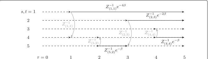
Figure2shows a simple example of this definition overlaid on the example of Fig.1.

2_{Allowing a negative absolute temperature (Ramsey1956),β= −∞andβ= ∞respectively correspond to “absolute}

Fig. 2Entries ofP(β)_(C,a,1)not in{0, 1}forC:= {(1, 4, 1),(5, 4, 2),(2, 5, 3),(4, 3, 4)}anda= {0, 5}are indicated

along with solid arcs (gray for spatial arcs; black for temporal arcs); unit entries correspond to dashed arcs

The specific formulae of (4) arise from the four identified constraints above rather than from arbitrary choices.

In particular, the requirementa∩τ(C) = ∅ensures that the Markov chain defined by (4) has exactlyn absorbing states. Each of these has the form(v,am) and a corre-sponding “emitting” state(v,am−1), and a natural quantity to consider is the probability Q(β)_(C,a,m)(v,w)of arriving at the absorbing state(w,am)after starting in the emitting state (v,am−1). We can straightforwardly compute this quantity using the so-called fundamen-tal matrix(Brémaud1999). Finally, the termτ₍@_a,v_m+₎mitigates artificial “boundary effect” behavior form=M.

Taken as a whole, (4) thus leads to a natural temporal coherence property and a straight-forward physical interpretation. Regarding the symmetries and invariants listed above, the terms equal to 1 and 0 in (4) merely codify i), while ii) is embodied in the following identity which can easily be verified from the construction of the probability transition matrices,Q(β)_(C,a,m).

Lemma 1If a0,a|a|−1∈a⊆a, then

Q(β)_(C,a,1)· · · · ·Q₍(β)_C,a,|a|−1)=Q(β)_(C,a,1)· · · · ·Q₍(β)_C,a,|a|−1). (5)

ProofThe lemma follows by applying the Kolmogorov-Chapman property to each of the inhomogeneous Markov chainsQ(β)_(C,a,·)andQ(β)_(C,a,·).

That is, for any DCNCand parameterβ, we have an associated temporally coherent family of time-inhomogeneous Markov chains. This lemma does not rely on the specific form of (4): the exp(−β ·τ) terms could be significantly changed without breaking property ii) above.3

Moreover, this form is necessary to jointly satisfy properties iii) and iv): i.e., memo-rylessness and self-consistency in the limitτ ↓ 0. (In particular, the self-consistency requirement prohibits multiplying the exponentials by some nontrivial constant.) That is, the form of (4) is dictated by the structure of a temporal digraph along with manifestly desirable symmetries.4

3_{That said, a dependence onτis necessary. In the context of intra-computer information flows, this time difference}

plausibly approximates (at least for small values) a linear function of the conditional Kolmogorov complexity of the intervening computation.

4_{We can generalize this construction to the related notion of a weighted DCN by normalizing the sum of outbound}

In the limitβ → ∞, the trajectories of the Markov model are so-calledgreedy walks (Saramäki and Holme2015), and more generally forβ >0, “spatial” transitions are pre-ferred over “temporal” transitions. Regardless of the value of β, we shall see that the temporal coherence of trajectories is captured more faithfully and conservatively in the Markov model than in series of “projected snapshots” that characterize earlier efforts such as Perra et al. (2012); Starnini et al. (2012); Rocha and Masuda (2014); Grindrod and Higham (2013); Valdano et al. (2015) to analyze DCNs through graph time series and/or provide a substrate for random walks. A recent notable work that develops techniques for special epidemiological models can be found in Valdano et al. (2018).

The preceding lemma facilitates a computational complexity analysis as a function ofa. WritingN:= |C|andM:= |a|, we suppose thatais approximately uniform in the sense thatC|[am,am+1) ≈ N/M, which also implies that|V(T(C|[am,am+1)))| ≈ 2(n+N/M).

The complexity of computingQ(β)_(C,a,m)is governed by a matrix division of the form(I− Q)\R, where here Qis the block of P(β)_(C,a,m) whose rows and columns both correspond to transient states, andRis the block whose rows and columns respectively correspond to transient and absorbing states. Since the numbers of transient and absorbing states are respectively approximatelyn+2N/Mand exactlyn, the complexity of computing (I−Q)\RisO(n(n+2N/M)ω−1), where we take matrix multiplication and inversion to have complexity exponentω > 2 (for dense unstructured matrices, in practiceω = 3). Because there areM−1 matrix multiplications, the computational complexity for the right hand side of (5) isO(Mn(n+2N/M)ω−1). Now arg minMMn(n+2N/M)ω−1 = 2(ω−2)N/n, and this value forMyields computational complexity which is nominally linear inN. Meanwhile, it only makes sense to takeM N/nif the complexity of the linear algebra involved is dominated by the rest of the computation. In other words, it is less expensive to invert and multiply many small matrices than to invert and multiply a few large matrices. Since takingMlarger yields a more detailed picture of the dynamics ofC, it is sensible to requireMto be (at least) on the order ofN/n.

We exhibit the basic mechanics of the model in the following

Example 1Consider once more the DCN shown in Fig.1. Letτj=j for1≤j≤4,ε1, a= {0, 2.5, 5}and a = {0, 5}. The entries of P₍(β)_C,a,1)are then as in Fig.2and (using·in matrices to denote 0 for clarity)

Q(β)_(C,a,1) = ⎛ ⎜ ⎜ ⎜ ⎜ ⎜ ⎜ ⎜ ⎝

eβ+1

(e4β_+1)(eβ₊₁₎ · e

5β

(e4β_+1)(eβ₊₁₎ e

4β

(e4β_+1)(eβ₊₁₎ ·

· 1

e2β₊₁ · · e

2β e2β₊₁

· · 1 · ·

· · eβ

eβ+1

1

eβ+1 ·

· · e2β

(eβ+1)2 e

β

(eβ+1)2 e

β₊₁

(eβ+1)2

⎞ ⎟ ⎟ ⎟ ⎟ ⎟ ⎟ ⎟ ⎠ = ⎛ ⎜ ⎜ ⎜ ⎜ ⎜ ⎜ ⎝ 1

e4β₊₁ · · e

4β e4β₊₁ · · 1 · · · · · 1 · · · · · 1 · · · · eβ

eβ+1 1

eβ+1

⎞ ⎟ ⎟ ⎟ ⎟ ⎟ ⎟ ⎠ · ⎛ ⎜ ⎜ ⎜ ⎜ ⎜ ⎜ ⎝

1 · · · ·

· 1

e2β₊₁ · · e

2β e2β₊₁

· · 1 · ·

· · eβ eβ+1

1

eβ+1 ·

· · · · 1

⎞ ⎟ ⎟ ⎟ ⎟ ⎟ ⎟ ⎠

so that with increasingβ(or equivalently, decreasing temperature) the likeliest transitions correspond to temporally coherent paths that greedily traverse spatial arcs. Now consider the digraph D with arcs(s(c),t(c))for c ∈ C and loops(v,v)for v ∈[n]. The adjacency matrix of D has nonzero entries in the same locations asQ(β)_(C,a,1), and also in the(2, 3)and (2, 4)locations. The(2, 3) and(2, 4)entries correspond to spurious temporally coherent paths inC. In particular,Qgives a more faithful description ofCthan D.

Although the context is quite different, the closest work to the construction of this section is Ser-Giacomi et al. (2015), which shows that the most probable paths in a Marko-vian model of a very complicated temporal network (viz., ocean water transport in the Mediterranean) suffice to describe the network’s key features. Other works have looked at higher-order models in discrete time as a way to finesse the challenges of continu-ous time modeling as discussed here (Lambiotte et al.2019; Rosvall et al.2014). Despite the many differences of detail, our own model likewise shows that the most probable paths/flows suffice for capturing the essential dynamics of directed contact networks. In particular, this includes flows that the model assesses as highly probable, but whose asso-ciated contact motifs occur infrequently (or perhaps just once in a given data set): in our experiments, such flows reliably capture anomalous and even malicious behavior (see, for example “Data reduction and anomaly detection” section).

Embeddability

It is natural to wonder under what if any circumstances the Markov chainQ(β)_(C,a,m) corre-sponds to a continuous-time Markov process. As it happens, this instance of theMarkov embeddabilityproblem Lencastre et al.2016) can be answered quite effectively (if not always affirmatively) for most situations of practical interest.

In the event that no two contacts are simultaneous, this problem reduces to the case of a single contact forn=2, which in turn follows from the following identity forp∈(0, 1), which can be verified by using the power series expansion for log:

log

1−p p

0 1

=log(1−p)·

1 −1 0 0

. (7)

On the other hand, simultaneous contacts are a possible obstruction to embeddability. Forn =2, a stochastic matrix is embeddable iff it has positive determinant. But a quick calculation forC := {(1, 2, 0),(2, 1, 0),(1, 2,τ),(2, 1,τ)}anda= {−1,τ/2, 2τ}shows that detQ(β)_(C,a,1)<0 forβ >0.

Proposition IV.3 of Lencastre et al. (2016) immediately yields a generalization of the preceding observations:

Proposition 1If T(C)is acyclic, thenQ(β)_(C,a,m)is embeddable.

Finally, when a Markov generator exists, the algorithm of §V.B of Lencastre et al. (2016) can be used to estimate it.

In this section, we sketch how the model of “Markov chain models for DCNs” section performs data reduction well enough to be used as a practical anomaly detector. For some additional background details of this analysis, see (Huntsman2018b).

We considered a DCNCformed fromN ≈ 3.4·106kernel-level events spanning a

period of four days and derived in turn from data produced by the CADETS tool (Jenkin-son et al.2017). Also, after curation, we obtained a setG⊂Cof 216 ground truth contacts that were distributed over 54 malicious exfiltration events.

At a high level, we mapped an event represented as

(timestamp,(process name,process identifier),event type,filename)

(where the “everything is a file” philosophy applies to the last entry, such as, for a fork event, the filename is the forked process identifier) onto

(process name,filename,timestamp),

or

(filename,process name,timestamp),

or both, depending on the semantics of event type. While many event typesemantics

included a natural and unambiguous (bi)directionality determining the mapping above, some did not, and in that case both contacts were conservatively included.

We obtained flows using the model of “Markov chain models for DCNs” section by

settingβto the mean inter-contact time (i.e., the proposed heuristic) and usedM=28423 windows of 10 s.

We letIˆ(m)denote the set of indices corresponding to sources or targets of flows span-ning themth time window that simultaneously fell above a flow probability threshold λ∈[ 0, 1] and below a per-window frequency thresholdμ∈[ 0, 1]. The setIˆ(m)is an esti-mate of the setI(m)of indices corresponding to sources or targets of ground truth events during themth time window.5

Using the estimated and ground truth index setsIˆ(m)andI(m), we defined two ver-sions of detection metrics. Suppressing the argumentmfor clarity, the “Boolean” version usesTrue= :=1 andFalse= ⊥:=0 so that

δbool+ :=

ˆ

I=∅∧Iˆ∩I =∅;

δ_bool⊥+ := Iˆ =∅∧Iˆ∩I=∅;

δ_bool⊥− :=

ˆ

I=∅∧[I=∅] ;

δbool− :=

ˆ

I =∅∧[I=∅] . (8)

The natural number analogues of (8) are

δnat+:=Iˆ∩I; δnat⊥+:=Iˆ∩Ic; δ⊥−nat :=Iˆc∩I; δnat− :=Iˆc∩Ic. (9)

From these we get in turn the usual detection metrics shown in Figs.3 and4, i.e. true positive rate (or recall) and false positive rate

5_{This construction was necessary because in many cases the source or target of a ground truth event did not exist. For}

example, the userspace commandshostnameandput /tmp/netreconcorrespond to the

TPR :=

mδ+(m)

mδ+(m)+

mδ⊥−(m)

; FPR :=

mδ⊥+(m)

mδ⊥+(m)+

mδ−(m)

, (10)

and positive predictive value (or precision) and negative predictive value

PPV :=

mδ+(m)

mδ+(m)+

mδ⊥+(m)

; NPV :=

mδ−(m)

mδ⊥−(m)+

mδ−(m) . (11)

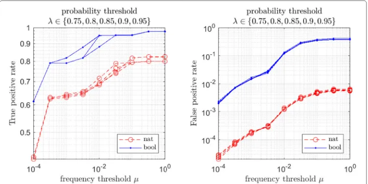
From Figs.3and4, we can see that the results were insensitive to the probability thresh-oldλ.6 Similarly, a cursory analysis indicated broad insensitivity to the value ofβ over several orders of magnitude, a fact attributable to information flow probabilities that tended to be either very near or bounded away from 1. This also underlies the insensitivity with respect to the probability thresholdλ. For the valueμ = 10−3, a majority of mali-cious events were detected with a false positive rate below 2 percent (by either version of the metrics).

The results indicate that the Markov model is a sufficiently effective data reduction technique (in particular, the negative predictive value is essentially perfect) to be a useful anomaly detector. In fact, of the 57 (out of 418) files which are targets of high-probability potential information flows in the model, 27 fell below theμ=10−3level and had back-tracks (King and Chen2005) with fewer than 20 (or for that matter, 90) vertices. From these 27, 6 (in 3 pairs) corresponded to the 3 executables which the malicious attacker wrote to/tmpfrom its initial foothold.

Taint bounds

The notions ofdynamic taint analysis (Schwartz et al.2010) andprovenance(Cheney

et al.2013) inform the context where a DCN models information flow in a

computa-tional environment. The analytic problems corresponding to these notions are generically undecidable. With this in mind, we introduce the idea oftaint bounds, wherein correct nontrivial bounds on the information flow are maintained.7We formalize this idea here before showing its utility as a practical guide to producing effective data-reducing path abstractions.

Letρbe a nontrivial binary relation on a finite setX such that the transitive closure ρ+_{is irreflexive (such relations have been calledsuperirreflexive(Fla˘ska et al.2007)), and}

hence also a strict partial order. Letγ : X →[ 0,∞)and define thelower taint boundα andupper taint boundβforx∈Xas follows:

α(x) :=

x1ρx

α(x1)

∧γ (x); (12)

β(x) :=

x1ρx

β(x1)

∧γ (x) (13)

where a ∧ b = min(a,b) in this section. Here we note that the standard

inter-pretation here is that not only minima but also summation over the empty set yield∞.

6_{In more delicate situations, the approach of Huntsman (2018a) offers a principled solution to the problem of}

thresholding.

7_{Notwithstanding their fundamentally dynamic character, these bounds may be regarded as having a loose analogue in}

Fig. 3True (left) and false (right) positive rates as defined in (10) for APT detections using the model of “Markov chain models for DCNs” section and as functions of a per-window frequency thresholdμand for varying flow probability thresholdsλ

Lemma 2αandβare well-defined; moreover,α≤β≤γ and

α(x)=

⎛

⎝

xρ+x γ (x)

⎞

⎠_{∧γ (}x). (14)

ProofBy lemma 3.5 of Fla˘ska et al. (2007), a binary relationρis superirreflexive iff the digraph corresponding toρis acyclic. Since by assumptionρis nontrivial andXis finite, there exists somej<∞such thatρ◦(j+1)_=∅andρ◦j_{=∅, where the composition ofρ} with itself is indicated. Furthermore, superirreflexivity implies irreflexivity.

Therefore, the recursion implicit in (12) terminates and we have

α(x)=

⎡

⎣

x1ρx

⎛ ⎝ ⎡

⎣

x2ρx1

. . .

⎛ ⎝ ⎡

⎣

xj+1ρxj

α(xj+1)

⎤ ⎦_{∧γ (xj)}

⎞ ⎠_{. . .}

⎤ ⎦_{∧γ (x1)}

⎞ ⎠ ⎤

⎦_{∧γ (x)}. (15)

But_xj+1ρxjα(xj+1)= ∞andxkρ◦kxfor allk∈[j], so

α(x)=

⎛

⎝

x1ρ◦jx

γ (xj) ⎞ ⎠_{∧ · · · ∧}

⎛

⎝

x1ρ◦1x

γ (x1)

⎞

⎠_{∧γ (x)=} ⎛

⎝

xρ+_x γ (x₎

⎞

⎠_{∧γ (x)}. (16)

Similarly, the recursion implicit in (13) also terminates, though in this case without any additional simplification. The boundsα≤β≤γ follow.

For a DCNDsuch thatτ is injective, a natural choice forρ isc1ρc ⇐⇒ (t(c1) = s(c))∧(τ(c1) < τ(c)). Note that this relation is superirreflexive.

Example 2Consider once more the DCN depicted in Fig.1andρas defined immediately above. The only nontrivial taint bounds are for the last contact: we have thatα(4, 3,τ4)= (γ (1, 4,τ1)∧γ (5, 4,τ2))∧γ (4, 3,τ4)andβ(4, 3,τ4)=(γ (1, 4,τ1)+γ (5, 4,τ2))∧γ (4, 3,τ4). If for 3 ≤ j ≤ J we add to this DCN the contacts (3, 4,τ2j−1) and(4, 3,τ2j) with τk strictly increasing, then the result is a DCN with2J contacts andα(·,·,τk)andβ(·,·,τk) nonincreasing for k>4.

However, in practiceτneed not be injective, and in fact this is often the case for kernel-level information flows (timestamps of system-kernel-level activity in computers or network interfaces are generally precise only to milliseconds or at best microseconds, and getting higher precision generally entails a heavy burden or can even be practically infeasible, depending on the detailed context). Indeed, for a distributed system, even the synchro-nization of clocks can become an issue, and so it is desirable to have a relationρ that accounts for more structural details. The problem is highlighted by considering directed

acyclic graphs (DAGs) rather than DCNs: for a DAG D, the natural choice for ρ is

uρviffu precedes v. However, this does not generalize to arbitrary digraphs, which are the structures that essentially embody multiple contacts occurring at the same time.

This suggests two strategies: live with a fairly generic relationρand only seek to com-pute taint bounds when the digraph corresponding toρactually turns out to be acyclic, or build in mechanisms that enforce acyclicity (if these are artificial, we can provide warnings when they have any effect). Only the second of these strategies requires further comment here. One simple approach is to leverage some auxiliary strict order onX; another simple approach is to require a nonzero delay between contacts. In general, context will constrain and inform the construction ofρ.

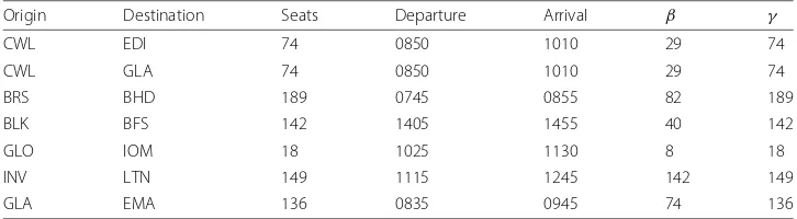
Table 1Taint bounds withβ < γfor UK flight data in Example3

Origin Destination Seats Departure Arrival _{β γ}

CWL EDI 74 0850 1010 29 74

CWL GLA 74 0850 1010 29 74

BRS BHD 189 0745 0855 82 189

BLK BFS 142 1405 1455 40 142

GLO IOM 18 1025 1130 8 18

INV LTN 149 1115 1245 142 149

GLA EMA 136 0835 0945 74 136

Let us consider each of these in turn. On the day in question, one flight arrives at CWL by 0820, and it has 29 seats. Two flights arrive at BRS by 0715, each with 41 seats. Two flights arrive at BLK by 1335, each with 20 seats. One flight arrives at GLO by 0955, and it has 8 seats. Three flights arrive at INV by 1045, with 34, 34, and 74 seats, respectively. Finally, one flight arrives at GLA by 0805, and it has 74 seats. The general pattern amongst these is evident by inspection: there are a few preceding flights inbound to the origin with less total capacity than the current flight.

The preceding example illustrates by way of analogy how differences betweenβ and

γ can serve as a preliminary indicator of anomalously asymmetric flows (which might

correspond to, for example, the original dissemination of material and/or unauthorized data exfiltration), particularly at vertices corresponding to sensitive objects or locations.

Renormalization

Forτ1 < · · · < τN ∈ R, consider the DCNC := {(1, 2,τj)}N_j=−₁1. It is of interest to try to associateCwith a single coarse-grained or “renormalized” contact using the Markov model of “Markov chain models for DCNs” section. WritingQ=Q(β)_{(C,{−∞,τ}

N},1), we have that

Q11=

j e−δj

1+e−δj, (17)

whereδj:=β(τj+1−τj). If we pickso that

Q11=: e−

1+e− (18)

then

=log ⎛

⎝

j

[eδ_j +1]−1 ⎞

⎠. (19)

We want 0≤≤_jδj, so that the notional renormalized contact(1, 2,τN−)can replaceCin a self-consistent way. While the first inequality holds, the second is equivalent to_j[eδj+_1]≤

jeδj+1, which is impossible forβ >0. That is, our goal of associating

Cwith a single renormalized contact is generally impossible.

their fixed points. We also note that renormalization ideas have been applied to undi-rected networks with specific structures (Barrat and Cattuto2013; Karschau et al.2018;

Newman and Watts1999).

For a theory determined by a functionf(x;θ) of dataxand parametersθ, and given a suitable coarsening operator C, if there exists a function g such that f(x;θ) = f(C(x);g(θ)), then the theory is calledrenormalizable.8In our setting, a probability cut-off takes the role off; the underlying DCN takes the role ofx; the parameterβ = θ is computed from the dataxaccording to a fixed heuristic; and the coarsening operatorC is realized by the Markov model of “Markov chain models for DCNs” section along with a fixed heuristic for its remaining parameters - for instance, we can fix the number of contact times per window (with an exception provided for the last window). The use of fixed heuristics yields a RG transformation on DCNs that renormalizes probable flows into contacts in a given time window.

Iterating the RG transformation along these lines leads to an "ultraviolet cutoff" at which the process stops, essentially sublimating temporal data into a single weighted digraph. While there is a great deal of freedom in its precise specification, such an RG transformation and fixed point is surely of interest for summarizing complex DCNs.

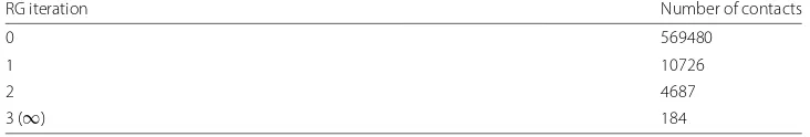
In Table2, we show the sizes of DCNs obtained through such RG transformations up to a fixed point in an experiment on data similar to that described in “Data reduction and anomaly detection” section. Of the final 184 renormalized contacts, at least 8% appeared to be associated with malicious activity.

Clustering

The problem of clustering in digraphs is much more delicate than its analogue for the undirected case (Malliaros and Vazirgiannis2013). It should therefore come as no sur-prise that the problem of clustering in DCNs is more challenging than either clustering in digraphs or in undirected temporal networks. Indeed, most of the approaches purport-ing to address clusterpurport-ing in temporal networks in the literature (cf. §4.11 of (Holme2015), §4.12 of Masuda and Lambiotte (2016) or Speidel et al. (2015)) actually cluster in time series of graphs, not the more granular notion of a DCN.

A sensible step forward is to consider the temporal digraphT(D)of a DCND. As an “almost acyclic” digraph, it might seem natural to try to apply techniques such as those detailed in Malliaros and Vazirgiannis (2013) directly toT(D). While this would offer the prospect of retaining qualitative temporal structure, it still ignores the quantitative temporal details; furthermore, it is far from evident how to remove any cycles that might (and in practice frequently do) occur. We seek instead a controlled way to coarse-grain this temporal information independent of the approach in “Renormalization” section.

We note that clustering for temporal networks is a topic of much current interest (Bas-sett et al.2013; Bazzi et al.2016; Gauvin et al.2014; Sarzynska et al.2015) seeing as the dynamics of communities within social networks and other applications are relevant to current social media and related topics. However, our focus here is an on the specific structure of directed contact networks which has not been specifically studied to our knowledge before.

8_{Renormalizable theories in physics (and their fixed/critical points) are of great interest: indeed, renormalizability is}

Table 2Reduction of data similar to that described in “Data reduction and anomaly detection” section under RG transformations

RG iteration Number of contacts

0 569480

1 10726

2 4687

3 (∞) 184

Clustering techniques leveraging (5)

The time-inhomogeneous Markov chain (5) provides a platform for any number of

capabilities, not least clustering. Before plunging ahead, the taxonomy of Malliaros and Vazirgiannis (2013) for digraph clustering suggests some guiding principles:

1. Any clustering technique ought to directly exploit the probabilistic framework that (5) offers and seek to avoid any additional model features unless they are necessary. This principle discourages–but of course does not completely rule out–techniques that require for example random walks generated by an ergodic transition matrix, which would in turn require incorporating a “teleportation” deviceà la PageRank. Techniques that require a unique and/or nondegenerate stationary distribution are therefore also discouraged by this principle. Such discouraged techniques include (following the precise enumeration in table 2 of Malliaros and Vazirgiannis (2013)) symmetrization and random walk simulations, LinkRank, directed Laplacians, two-step random walks, message passing, and Infomap. Meanwhile, many other techniques do not exploit (5) at all and should be completely ruled out: for example, network embedding, bipartite modularity, a modified adaptive genetic algorithm, semi-supervised learning, directed modularity, directed Gaussian random network, overlapping modularity, local modularity, cuts, attraction/repulsion, local

partitioning, directed clique percolation, local density, mixture models, and community kernels.

2. The techniques in Malliaros and Vazirgiannis (2013) not discouraged or completely ruled out by the immediately preceding considerations essentially amount to coclustering (or the closely related notion of “blockmodels”). Among coclustering approaches, we single out (Ge et al.2003; Chakrabarti2004; Rohe et al.2016) as holding particular interest. (Ge et al.2003) focuses on reducing the number of states of a Markov chain estimated directly from a sample trajectory (and is thus not manifestly suitable in our context, where the data is a sequence of contacts rather than a sequence of vertices), while (Chakrabarti2004; Rohe et al.2016) explicitly address unweighted digraphs. (Ge et al.2003; Rohe et al.2016) cluster singular vectors of a suitable matrix, whereas (Chakrabarti2004) optimizes a minimum description length criterion for coclustering. Bearing all this in mind, a reasonable strategy would be to look for opportunities to evaluate the singular value

decomposition or an information-theoretical compression of a suitable matrix. At the same time, the notion of stochastic equivalence (Holland et al.1983) leveraged by (Rohe et al.2016) appears particularly relevant: verticesv and w are stochastically equivalent for (5) iffQv·=Qw·andQ·v,Q·w, where we use a shorthand. We shall

Intuitively, a time-dependent clustering for vertices of a DCN that models the flow of some quantity ought to be determined by a metric involving the probabilities of transi-tions to and from states. Letddenote an arbitrary metric on probability distributions and writeQfor a matrix such as in (5). If we are only concerned with the probabilities of transitions from states, then it suffices to consider

d(v,w):=d(Qv·,Qw·). (20)

If instead we are only concerned with the probabilities of transitions to states, the situ-ation is more delicate. The reason is that in general (5) will not yield a very well-behaved Markov chain, even apart from any time-inhomogeneity. For example, reducibility is com-mon in practice. This means that the classical notion of time reversal for the chain is not well-defined, which complicates any attempt to consider the probabilities of transi-tions to states. Nevertheless, it is easy to construct an essentially unique time reversalD←

of the underlying DCNDby merely swapping sources and targets and replacingτ with

τ∗−τfor any fixedτ∗∈R. WritingQ←for a matrix obtained by applying (5) toD←, the time-reversed analogue of (20) is

d←(v,w):=d(Q_v←_·,Q←_w·). (21)

Meanwhile, if we are concerned with the probabilities of transitions both to and from states, it is both natural and easy to consider for 0<q<∞(with an extension toq= ∞) an induced metric (and the metric property itself is easy to show) of the form

d↔_q (v,w):=[(d(v,w))q+(d←(v,w))q]1/q. (22)

Any of the preceding metrics (20), (21), or (22) lend themselves straightforwardly to various clustering techniques.

Example 4If d is the total variation or Hellinger distance, then the metric (20) takes values in the unit interval. It is then reasonable to automatically select a cutoff for a hierarchical clustering technique along the same lines as described in “Data reduction

and anomaly detection” section, possibly after some rescaling. Here, we will consider total

variation distance and use single linkage clustering.

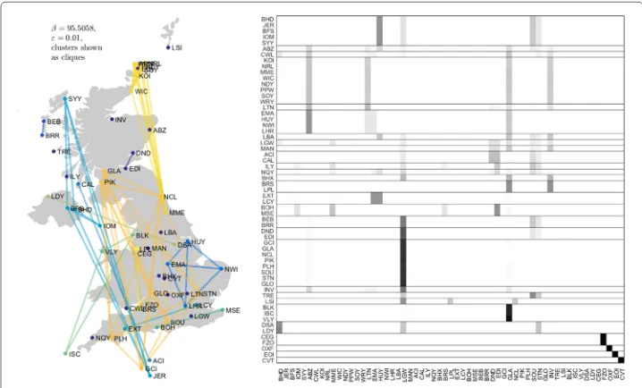
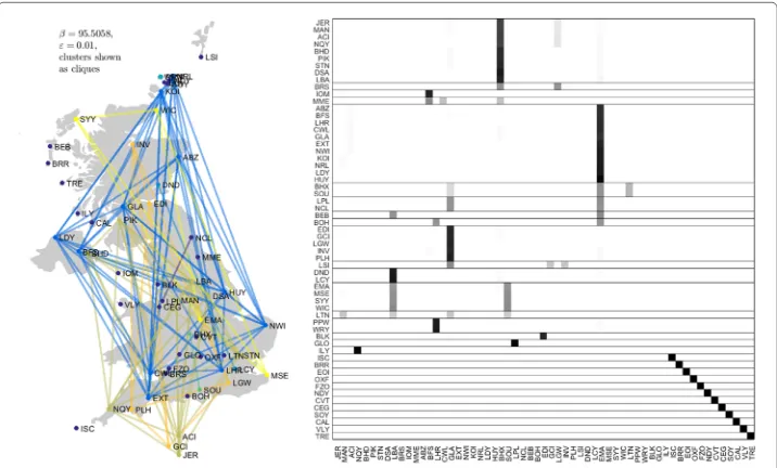
Recall the DCN of nonstop UK domestic flights described in “Taint bounds” section, but now over the entire week of 18 October 2010. Because this DCN has a rather idiosyncratic bipartite structure, it is not particularly instructive to look at its local temporal behavior à la (5): many of the transitions will be between airports and flights or conversely, rather than between two airports. Therefore, we consider the DCN a day at a time to avoid “getting stranded on a plane”. The results are shown in Figs5,6,7,8,9,10and11.

For Monday, some of the likeliest transitions are as follows:

• The transitions from CEG and FZO to FZO arise from a sequence

CEG→FZO→CEG→FZO of three chartered flights between these airports, which host Airbus facilities and have no other scheduled passenger flights.

Fig. 5Clusters from UK flight data for Monday, 18 October 2010 obtained using total variation distance in (20) and single linkage, with a dendrogram cutoff automatically selected along the lines mentioned in “Data reduction and anomaly detection” section. (L) Clusters displayed as cliques. (R) Transition matrix for

β=1/τandε=10−2, with entries indicated by grayscale and indices/airports permuted to reflect clusters, which are themselves delineated by horizontal lines

at 1300 and taking the shortest possible (even instantaneous) layovers, we have the sequence of nominally connecting flights

GLA

1315 → 1425

LTN

1500 → 1610

GLA

1610 → 1730

LCY

1735 → 1910

EDI

1920→ 2020

MAN

2020 → 2120

SOU

that terminates at SOU when there are no more departing flights for the day.

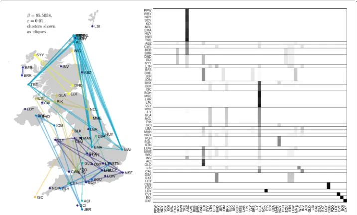
Fig. 7Clusters from UK flight data for Wednesday, 20 October 2010; otherwise as in Figure5. Cluster colors only distinguish clusters from each other and do not suggest affinity across days

• The transitions from EMA, HUY, and NWI to ABZ arise as follows. The first flights departing EMA, HUY, and NWI each arrive at ABZ between 0800 and 0810; meanwhile, the first flight departing ABZ not earlier than 0800 departs to MME at 0820. Taking shortest possible layovers as above eventually terminates at ABZ when there are no more departing flights for the day.

The “greedy” connections of the sort above become less likely asβdecreases.

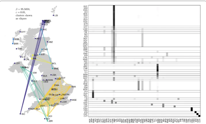
Fig. 9Clusters from UK flight data for Friday, 22 October 2010; otherwise as in Fig.5. Cluster colors only distinguish clusters from each other and do not suggest affinity across days

Remarkably, there is a considerable amount of geographic coherence to the clusters on weekdays, particularly on Friday. For example, even the two geographically largest clusters in the center panel of Fig.5 consist entirely of airports on the periphery of the UK and Crown dependencies. As another example, the airports in Orkney with service (viz., KOI, NDY, NRL, PPW, SOY, and WRY) are part of a single, geographically local cluster.9

The time reversal (not shown) is less coherent, probabilistically and geographically. This highlights a critical distinction between DCNs with scheduled versus observed contacts. The former will generally correspond to something like a transportation network that is specifically engineered to facilitate certain connections (this in turn highlights that the UK domestic flight data is really a superposition of DCNs corresponding to individual airlines, with codeshares serving to add further complexity). It seems plausible that this distinction underlies the very limited degree of commonality between the forward and time-reversed clusters.

Remarks

The model of “Markov chain models for DCNs” section exhibits a very sensitive depen-dence on the structure of the underlying DCN. In experiments not detailed here, we have seen that inserting just 1% of uniformly random contacts seriously degrades the model’s data reduction and anomaly detection characteristics. Rather than being a shortcoming, this behavior demonstrates that the model actually captures delicate yet critical aspects of flows from contact data.

An interesting perspective on this model is that it yields a time-varying geometry once a metric on probability distributions is chosen. Using the induced metric to assess the

9_{As an amusing aside, the shortest scheduled passenger flight in the world is between PPW and WRY: it has been}

Fig. 10 Clusters from UK flight data for Saturday, 23 October 2010; otherwise as in Fig.5. Cluster colors only distinguish clusters from each other and do not suggest affinity across days

model dynamics is worth examining in future work. In a similar vein, analyzing the vari-ation of informvari-ation (Meil˘a2007) between subsequent clusterings would give additional principled insight into the behavior of DCNs.

Regarding the taint bounds of “Taint bounds” section, we note that using alternative arithmetics/semirings along similar lines is also of interest, such as the so-called log and Viterbi semirings.

Abbreviations

DAG: directed acyclic graph (In “Taint bounds” section and “Clustering” section we make extensive use of International Air Transport Association airport codes, for which seehttps://www.iata.org/services/Pages/codes.aspx.); DCN: directed contact network; FPR: false positive rate; NPV: negative predictive value; PPV: positive predictive value (or precision); RG: renormalization group; TPR: true positive rate (or recall); UK: United Kingdom

Acknowledgements

We thank Yingbo Song, Rob Ross, and Mike Weber for many helpful discussions as well as creating the summary and ground truth data used in “Data reduction and anomaly detection” section.

Authors’ contributions

GC conceived of and prototyped the techniques discussed in “Taint bounds” section, provided advice and comments on the subject matter of the entire paper, and edited the manuscript. SH conceived of the model in “Markov chain models for DCNs” section, performed the data analyses presented in the paper, and wrote the manuscript. Both authors read and approved the final manuscript.

Funding

This material is based upon work supported by the Defense Advanced Research Projects Agency (DARPA) and the Air Force Research Laboratory (AFRL). Cybenko’s efforts in this work were also partially supported by ARO MURI Grant W911NF-13-1-042. Any opinions, findings and conclusions or recommendations expressed in this material are those of the author(s) and do not necessarily reflect the views of DARPA, the US Army or AFRL.

Availability of data and material

Non-public datasets used and/or analysed during the current study are available from the corresponding author on reasonable request.

Competing interests

The authors declare that they have no competing interests.

Author details

1_{Thayer School of Engineering, Dartmouth College, Hanover, NH 03755, USA.}2_{BAE Systems FAST Labs, 4301 North}

Fairfax Drive, Arlington, VA 22203, VA, USA.

Received: 11 March 2019 Accepted: 10 September 2019

References

Bang-Jensen J, Gutin G (2009) Digraphs: Theory, Algorithms and Applications. 2nd. Springer, LOndon.https://doi.org/10. 1007/978-1-84800-998-1

Barenblatt GI (2003) Scaling, Cambridge.https://doi.org/10.1017/cbo9780511814921

Barrat A, Cattuto C (2013) Temporal networks of face-to-face human interactions. In: Temporal Networks. Springer, Berlin. pp 191-216

Bassett DS, Porter MA, Wymbs, NF Grafton ST, Carlson JM, Mucha PJ (2013) Robust detection of dynamic community structure in networks. Chaos: Interdisc J Nonlinear Sci 23(1):013142

Bazzi M, Porter MA, Williams S, McDonald M, Fenn DJ, Howison SD (2016) Community detection in temporal multilayer networks, with an application to correlation networks. Multiscale Modeling Simul 14(1):1-41

Bianchi et al. FM (2016) Identifying user habits through data mining on call data records. Eng Appl Artif Intell 54:49-61 Brémaud P (1999) Markov Chains: Gibbs Fields, Monte Carlo Simulation, and Queues. Springer, New York

Chan SC, et al. (2017) Expressiveness benchmarking for system-level provenance. TaPP Chakrabarti D (2004) AutoPart: parameter-free graph partitioning and outlier detection. PKDD

Cheney J, Acar UA, Perera R (2013) Toward a theory of self-explaining computation. In: Tannen V, et al. (eds). Search of Elegance in the Theory and Practice of Computation. Springer

Flaška V, et al. (2007) Transitive closures of binary relations I. Acta Uni Carolinae - Math Phys 48:55

Gallotti R, Barthelemy M (2015) The multilayer temporal network of public transport in Great Britain. Sci Data 2:140056 Gallotti R, Barthelemy M (2015) The multilayer temporal network of public transport in Great Britain. Dryad Digit

Repository.https://doi.org/10.5061/dryad.pc8m3

Gauvin L, Panisson A, Cattuto C (2014) Detecting the community structure and activity patterns of temporal networks: a non-negative tensor factorization approach. PloS One 9(1):e86028

Ge X, Parise S, Smyth P (2003) Clustering Markov states into equivalence classes using SVD and heuristic search algorithms. AISTATS

Glazek K (2002) Selected Applications of Semirings. In: A Guide to the Literature on Semirings and their Applications in Mathematics and Information Sciences. Springer. pp 67–87.https://doi.org/10.1007/978-94-015-9964-1_6 Goldenfeld N (1992) How Phase Transitions Occur in Principle. In: Lectures on Phase Transitions and the Renormalization

Group. Addison-Wesley. pp 23–83.https://doi.org/10.1201/9780429493492

Grindrod P, Higham DJ (2013) A matrix iteration for dynamic network summaries. SIAM Rev 55:118 Holland PW, Laskey KB, Leinhardt S (1983) Stochastic blockmodels: first steps. Soc Netw 5:109 Holme P (2015) Modern temporal network theory: a colloquium. Eur Phys J B 88:234 Huntsman S (2018a) Topological mixture estimation. ICML

Jenkinson G, et al. (2017) Applying provenance in APT monitoring and analysis. TaPP

Karschau J, Zimmerling M, Friedrich BM (2018) Renormalization group theory for percolation in time-varying networks. Sci Rep 8(1):8011

King ST, Chen PM (2005) Backtracking intrusions. ACM Trans Comp Sys 23:51

Lambiotte R, Rosvall M, Scholtes I (2019) From networks to optimal higher-order models of complex systems. Nat Phys 15(4):313–320.https://doi.org/10.1038/s41567-019-0459-y

Lencastre P, et al. (2016) From empirical data to continuous Markov processes: a systematic approach. Phys Rev E 93:032135

Malliaros FD, Vazirgiannis M (2013) Clustering and community detection in directed networks: a survey. Phys Rep 533:95–142

Masuda N, Lambiotte R (2016) Models of temporal networks. In: A Guide to Temporal Networks. World Scientific.https:// doi.org/10.1142/q0033

Meil˘a M (2007) Comparing clusterings-an information based distance. J Mutlivariate Anal 98:873

Newman ME, Watts DJ (1999) Renormalization group analysis of the small-world network model. Phys Lett A 263(4-6):341–346

Nielson F, Nielson HR, Hankin C (2010) Principles of Program Analysis. Springer, Berlin

Perra N, et al. (2012) Random walks and search in time-varying networks. Phys Rev Lett 109:238701

Ramsey NF (1956) Thermodynamics and statistical mechanics at negative absolute temperatures. Phys Rev 103:20 Rocha LEC, Masuda N (2014) Random walk centrality for temporal networks. New J Phys 16:063023

Rohe K, Qin T, Yu B (2016) Co-clustering directed graphs to discover asymmetries and directional communities. Proc Nat Acad Sci 113:12679

Rosvall M, Esquivel AV, Lancichinetti A, West JD, Lambiotte R (2014) Memory in network flows and its effects on spreading dynamics and community detection. Nat Commun 5:4630

Saramäki J, Holme P (2015) Exploring temporal networks with greedy walks. Eur Phys J B 88:334

Sarzynska M, Leicht EA, Chowell G, Porter MA (2015) Null models for community detection in spatially embedded, temporal networks. J Compl Netw 4(3):363–406

Schwartz EJ, Avgerinos T, Brumley D (2010) All you ever wanted to know about dynamic taint analysis and forward symbolic execution (but might have been afraid to ask). In: 2010 IEEE Symposium on Security and Privacy.https://doi. org/10.1109/sp.2010.26

Ser-Giacomi E, et al. (2015) Most probable paths in temporal weighted networks: an application to ocean transport. Phys Rev E 92:012818

Speidel L, Takaguchi T, Masuda N (2015) Community detection in directed acyclic graphs. Eur Phys J B 88:203 Starnini M, et al. (2012) Random walks on temporal networks. Phys Rev E 85:056115

Valdano E, Poletto C, Colizza V (2015) Infection propagator approach to compute epidemic thresholds on temporal networks: impact of immunity and of limited temporal resolution. Eur Phys J B 88:341

Valdano E, Fiorentin MR, Poletto C, Colizza V (2018) Epidemic threshold in continuous-time evolving networks. Phys Rev Lett 120(6):068302

Publisher’s Note