O R I G I N A L A R T I C L E
Open Access
The Balassa-Samuelson effect reversed:
new evidence from OECD countries
Matthias Gubler
1*and Christoph Sax
2Abstract
This paper reconsiders the Balassa-Samuelson (BS) hypothesis. We analyze an OECD country panel from 1970 to 2008 and compare three data sets on sectoral productivity, including newly constructed data on total factor productivity. Overall, our within- and between-dimension estimation results do not support the BS hypothesis. For the time since the mid-1980s, we find a robust negative relationship between productivity in the tradable sector and the real exchange rate, even after including the terms of trade to control for the effects of the home bias. Earlier, supportive findings may depend on the choice of the data set and the model specification.
Keywords: Real exchange rate, Balassa-Samuelson hypothesis, Panel data estimation, Terms of trade
JEL classification: F14, F31, F41
1 Introduction
The Balassa-Samuelson (BS) hypothesis—stated by both
Balassa (1964) and Samuelson (1964), with a research
precedent in the work of Harrod (1933)—is one of the
most widespread explanations for structural deviations
from purchasing power parity (PPP)1.
According to the BS hypothesis, differences in the pro-ductivity differential between the non-tradable and the tradable sector lead to differences in price levels between countries when converted to the same currency. The hypothesis assumes that the law of one price for trad-able goods holds. Ceteris paribus, a productivity increase in tradables raises factor prices, i.e., wages, which in turn leads to higher prices of non-tradables and thus to an appreciation of the real exchange rate. In contrast, when the relative productivity of non-tradables increases, marginal cost cuts result in a lower price level.
The empirical evaluation of the BS hypothesis has gained a great deal of attention. As argued in a survey by
Tica and Druži´c (2006), the major share of the evidence
supports the BS model, but the strength of the results depends on the nature of the tests and set of countries analyzed2. In particular, cross-sectional studies have been
*Correspondence:[email protected]
1Swiss National Bank, Börsenstrasse 15, P.O. Box, 8022 Zürich, Switzerland Full list of author information is available at the end of the article
more successful in finding support for the BS hypothesis than panel data studies.
There are, however, several studies based on a disag-gregation of the tradable and non-tradable sector that find empirical support for the BS hypothesis (see, e.g., Calderón (2004); Choudhri and Khan (2005); Ricci et al. (2013) or Berka et al. (2018)). In particular, since sector-specific data for OECD countries on total factor produc-tivity (TFP) have become available, various studies have tested and confirmed the BS hypothesis using panel data
(De Gregorio et al. 1994; De Gregorio and Wolf 1994;
Chinn and Johnston1996; MacDonald and Ricci2007). All
these studies are based on the discontinued International Sectoral Database (ISDB) provided by the OECD.
This paper applies two panel cointegration models to estimate the long-run relationship between the real exchange rate and key explanatory variables, focusing on the effect of the TFP differential between tradables and non-tradables. Panel cointegration methods have become increasingly important in testing the BS hypothesis (Tica
and Druži´c2006). We use a novel OECD data set (PDBi)
with annual sector-specific TFP data from 1984 to 2008 to eliminate some of the shortcomings of the ISDB.
With this new data set, our estimations cannot con-firm the broad-based findings of previous research based
on the ISDB3. In fact, the results point to a negative
relationship between tradable productivity and the real exchange rate for OECD countries. In other words, for
the time since the mid-1980s, an increase in the
pro-ductivity oftradableshas given rise to adepreciationof
the real exchange rate. This finding is the opposite of what is claimed by the BS hypothesis, but it is in line with the empirical evidence for OECD countries docu-mented by Égert et al. (2006) and Fazio et al. (2007). Our analysis, however, differs from these studies in a
num-ber of dimensions, including the estimation methods4,
the data set, the sample period, and the set of OECD countries analyzed. Importantly, while these authors find a statistically significant negative relationship between thelaborproductivity of tradables and the real exchange rate, our analysis also relies on sector-specificTFP, which is the preferred measure for productivity as noted by
De Gregorio and Wolf (1994)5. However, we can confirm
this result when TFP is replaced by labor productivity (LP) using the OECD Structural Analysis (STAN) data set, which covers more countries and a longer time period, from 1970 to 2008. A rigorous analysis reveals that the finding of a negative coefficient on the productivity in the tradable sector for the time since 1984 is robust against the choice of the productivity measure (TFP or LP), the choice of the country sample, the precise start of the sample period, the exact model specification, and the inclusion of additional explanatory variables. Moreover, it seems that the negative effect of tradable productivity on the real exchange rate has strengthened over time. Our analysis further indicates that the choice of the model specifica-tions matters for the finding as to whether the empirical relationship between the productivity of tradables and the real exchange rate is negative or positive for the time period from 1970 to 1992, using the ISDB.
So far, the literature has primarily proposed devia-tions from the law of one price, such as a home bias in consumption preferences, as a possible mechanism for this reversed BS effect6. Benigno and Thoenissen (2003) develop a new open economy model in which a TFP shock in the tradable sector weakens the real exchange rate because the effect of the decrease of the price of its traded goods relative to that abroad dominates the effect of the increase of the relative price of non-traded goods7. More recently, Berka et al. (2018) provide a detailed break-down of the real exchange rate based on a New Keynesian model. In particular, they show that the traded goods real exchange rate depends on three factors: (1) differ-ences in relative non-traded goods prices across countries capturing distribution costs, (2) terms of trade (ToT) cap-turing home bias in preferences, and (3) deviations from the law of one price as deviations between the foreign price of identical goods relative to the home price. Thus, the authors distinguish between the effects of ToT and the explicit law of one price and assume that the latter
holds8. We adopt this assumption because the
aggrega-tion level of our data set does not allow us to consider
this third factor in the estimations. Berka et al. (2018) then show that relative non-tradable productivity, relative trad-able productivity, and ToT drive the overall real exchange rate. Therefore, we use ToT to control for the impact of movements in relative export to import prices on the real exchange rate. However, the inclusion of ToT does not change the significant negative relationship between the productivity of tradables and the real exchange rate. This result suggests that a productivity increase in the trad-able sector can lead to a decrease in the relative price of non-traded goods9. Gubler and Sax (2014) provide a static general-equilibrium framework with skill-based techno-logical change (SBTC), in which higher productivity in the tradable sector can lower wages, which in turn leads to lower prices of non-tradables and thus to a
deprecia-tion of the real exchange rate. Berka et al. (2018) show
that ToT are closely related to the relative unit labor costs (ULC) and propose to replace ToT with unit labor costs because the use of the ToT raises conceptual and empiri-cal difficulties. Therefore, we replace ToT with ULC in a robustness check. The negative relationship between trad-able productivity and the real exchange rate remains in force.
On the other hand, the connection between non-tradable productivity and the real exchange rate is not robust. Our robustness tests reveal that severe outlier dependency exists for the traditional Balassa-Samuelson
finding regarding non-tradables. In particular, Japanese
labor productivity in the non-tradable sector strongly weakens the estimated BS effect. For the time period from 1970 to 1992, the coefficient even significantly changes its sign once Japan is included.
Finally, with the exception of the terms of trade, our estimation results indicate that the explanatory power of further control variables discussed in the literature is weak or not robust.
The remainder of this paper is organized as follows.
Section2presents the data. We outline the methodology
in Section3and show the results in Section4. Section5
concludes.
2 Data
The data for the 18 major OECD countries included in our data set stem from different data sets of the IMF, OECD, World Bank, and the Penn World Tables. Depending on the estimation, the country sample has to be reduced
mainly because not all data are available10. A detailed
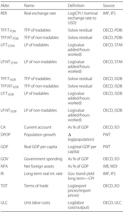
description of all variables is given in Table 1 and in
Appendix1.2.
To test the BS hypothesis, we condition the real exchange rate on productivity measures for both the trad-able and the non-tradtrad-able sector as well as on control vari-ables. The choice of the dependent variable is discussed
Table 1Description and construction of the variables
Abbr. Name Definition Source
RER Real exchange rate Log(CPI / nominal exchange rate to USD)
IMF, IFS
TFP.TPDBi TFP of tradables Solow residual OECD, PDBi
TFP.NTPDBi TFP of non-tradables Solow residual OECD, PDBi
LP.TSTAN LP of tradables Log(value added/hours worked)
OECD, STAN
LP.NTSTAN LP of non-tradables Log(value added/hours worked)
OECD, STAN
TFP.TISDB TFP of tradables Solow residual OECD, ISDB
TFP.NTISDB TFP of non-tradables Solow residual OECD, ISDB
LP.TISDB LP of tradables Log(value added/hours worked)
OECD, ISDB
LP.NTISDB LP of non-tradables Log(value added/hours worked)
OECD, ISDB
CA Current account As % of GDP OECD, EO
DPOP Population growth
log(population) PWT
GDP Real GDP per capita Log(real GDP per capita)
PWT
GOV Government spending As % of GDP OECD, EO
NFA Net foreign assets As % of GDP WB, WDI
RI Long-term real int. rate Gov. bond yield long term—CPI
IMF, IFS
TOT Terms of trade Log(export
prices/import prices)
OECD, EO
ULC Unit labor costs Log(labor
cost/output)
OECD, ULC
productivity data are separately examined in Section2.2.
All other exogenous variables are discussed in Section2.3. The time series properties of the variables are assessed in Section2.4.
2.1 Dependent variable: real exchange rate
We use the logarithm of the unweighted real exchange rate (RER) as the dependent variable in our estimation equations and define it such that an increase represents an appreciation. In principle, the real exchange rate can only be computed towards a reference currency. However, since we use time fixed effects throughout our analysis, the choice of the reference currency does not impact the results11. Like for all variables in our analysis, the inclu-sion of time fixed effects is equivalent to subtracting the annual sample mean. This is also true in the presence of DOLS estimators, when differences of variables are
used in the regression. In this case, the inclusion of time fixed effects is equivalent to subtracting the annual sam-ple mean of the difference. The advantage of not using a reference country is that it allows us to keep all available countries in the sample.
An extensive body of the empirical literature uses
effective real exchange rates (see, e.g., De Gregorio and
Wolf (1994); Calderón (2004) or Ricci et al. (2013))
that are weighted by the share of exports. Effective real exchange rates have the advantage that there is no need to specify a reference country. While effective real exchange rates are a useful measure for competitive-ness, the share of exports seems not only irrelevant in our context but also misleading. If, for example, a coun-try changes its export destinations to countries with a weaker real exchange rate, effective real exchange rates would indicate a real appreciation, while, in fact, the country still has the same relative price level towards all countries12.
2.2 Productivity data
We use data on sectoral productivity from three data sets provided by the OECD. The first is a new data set on sectoral total factor productivity (TFP) com-puted by the OECD, called PDBi. PDBi extends the older PDB by providing annual sector-specific TFP num-bers for the time period from 1984 to 2008. Sectoral TFP is calculated as Solow residuals with the same method for all countries, using sectoral data on pro-duction, employment, capital stock, and the labor share of income. Capital stocks are estimated by applying the permanent inventory method, where streams of invest-ments are added, and a certain fraction of depreci-ation is subtracted each year (for more details, see Arnaud et al. (2011)).
A second data set, STAN, includes yearly data on sec-toral production and employment—and thus on labor productivity—but not on TFP. As the only data set, STAN covers a long time range, from 1970 to 2008, for many OECD countries.
To compare our findings with the existing studies (De
Gregorio et al.1994; De Gregorio and Wolf1994; Chinn
and Johnston1996; MacDonald and Ricci2007), sectoral
productivity data from the discontinued ISDB have been used as well. This old data set contains annual values on labor and total factor productivity—in principle from 1970 to 1997—but was discontinued before 1997 for most countries.
for the public sector in the ISDB have simply been based on labor inputs such that the estimates of productivity had very limited meaning. Moreover, in the ISDB, volumes were calculated using constant prices instead of chain-linking. Finally, capital stock estimates may have been calculated differently and in a non-standardized way in the ISDB13.
We use these three OECD data sets for the following reasons: first, sectoral productivity data from PDBi has, to our best knowledge, not yet been used in testing structural deviations from purchasing power parity (PPP). Second, it allows us to compare our results, which are based on STAN and ISDB, with several important contributions to the literature on the BS hypothesis. Third, our approach also allows us to shed some light on whether differences in the results stem from the choice of the productivity mea-sure (TFP or LP), the estimation period or the choice of the data set. In addition, important control variables such as the terms of trade or unit labor costs also stem from OECD databases.
The classification of the subsectors into tradable and non-tradable is done according to the following scheme:
agriculture14, manufacturing, and transport, storage,
and communications are classified as tradables; utilities (energy, gas, and water), construction, and social services (community, social, personal services) are non-tradables. Our division of the subsectors into tradable or
non-tradable sectors follows De Gregorio and Wolf (1994),
who defined a subsector as tradable if its share of exports in the total production exceeds 10% and as non-tradable
otherwise15. While no division has become standard in
the field (Tica and Druži´c 2006), studies based on data
from OECD countries usually refer to the division
pro-posed by De Gregorio and Wolf (1994) (see, e.g., Chinn
and Johnston (1996); MacDonald and Ricci (2007)). Like
MacDonald and Ricci (2007), we exclude mining and
busi-ness services16due to data availability and the distribution subsector (wholesale and retail trade) due to classification difficulties. Based on a simple theoretical model,
Mac-Donald and Ricci (2005) show that an increase in the
productivity of the distribution subsector can have an ambiguous effect on the real exchange rate because of its role in delivering intermediate inputs to firms and final goods to consumers17.
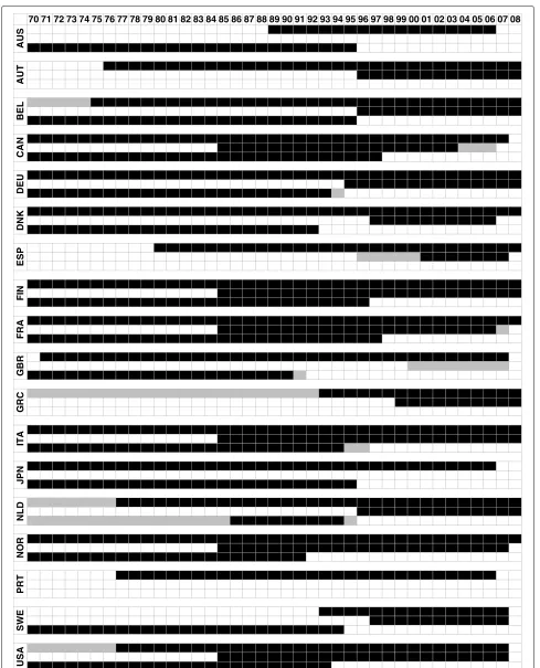
The tradable and non-tradable sectors, when classi-fied this way, are roughly equal in terms of the value added. Within the tradable sector, manufacturing is by far the largest subsector, representing 64% of the value added, whereas agriculture and transport as well as stor-age and communications amount to 11% and 24%, respec-tively. Among the non-tradables, social services (70%) outweigh construction (20%) and utilities (9%). Figure 2 in Appendix1displays the data availability in each of the three data sets.
Table2 shows the correlations between the three data
sets. The LP and TFP values from the ISDB are sim-ilar to the two newer data sets only in the tradable subsectors. In the non-tradable sectors, the correlations are lower (construction and utilities) or virtually non-existent (social services). To a lesser extent, this is also true for employment and value added. Possible rea-sons for these divergences have been discussed earlier in this section. On the other hand, the data from the PDBi on TFP are highly correlated with labor produc-tivity from the STAN data set. These correlations are present in all subsectors, although the values are some-what lower in the non-tradable subsectors. TFP data from ISDB and PDBi shows the lowest correlations. But again, the correlations are relatively high for agriculture and manufacturing, the main tradable sector. Unfortunately, there is only a low number of time-overlapping observa-tions on TFP from the PDBi and ISDB (see Figure 2 in
Appendix1), which may explain this result to a relevant
extent.
We consider TFP to be the preferred measure for
pro-ductivity. As noted by De Gregorio and Wolf (1994), the
average labor productivity increases much more quickly during economic downturns; hence, it is not a reliable indicator of sustainable productivity growth, which can affect the economy in the medium or long term. Nev-ertheless, there are some advantages of LP, and we will use the measure to check the robustness of our TFP results18.
2.3 Control variables
Along with the data on sectoral productivity, we take into account further potential determinants of the long-run
Table 2Median correlations across subsectors
AGR IND TSC EGW CST SOC
PDBi (TFP), STAN (LP) 0.95 0.97 0.92 0.95 0.93 0.84
ISDB (TFP), STAN (LP) 0.90 0.91 0.93 0.75 0.76 0.28
ISDB (TFP), ISDB (LP) 0.99 0.98 0.98 0.96 0.94 0.97
ISDB (TFP), PDBi (TFP) 0.70 0.70 0.45 0.45 0.45 0.45
ISDB (LP), STAN (LP) 0.90 0.88 0.88 0.72 0.77 0.27
ISDB (EMP), STAN (EMP) 0.91 0.98 0.91 0.89 0.99 0.45
ISDB (VA), STAN (VA) 0.91 0.95 0.89 0.72 0.93 0.45
Notes:The table contains median correlation coefficients between the variables in
real exchange rate, which have been proposed in the liter-ature. As described by De Gregorio and Wolf (1994) or Sax
and Weder (2009), among others, an improvement in the
terms of trade (TOT) allows a country to raise its imports for a given number of factor inputs in the export sec-tor. For example, a change in consumer preferences may shift global demand towards a specific country’s export goods. As a result, the good’s global price increases and, hence, the country’s real exchange rate appreciates. More-over, supply side changes may also affect the real exchange rate through movements in the terms of trade, for exam-ple, due to the home bias in consumption preferences
(see, e.g., Benigno and Thoenissen (2003); MacDonald
and Ricci (2007), Choudhri and Schembri (2010) or Berka et al. (2018)). Berka et al. (2018) show in a New Keynesian model that the terms of trade are closely related to the rel-ative unit labor costs (ULC). They propose to replace the terms of trade with unit labor costs because the use of the former raises conceptual and empirical difficulties. Unit labor costs are given as the ratio of total labor compensa-tion per hour worked to output per hour worked, and are thus directly comparable between countries. Most impor-tantly, the terms of trade and the real exchange rate are endogenous relative prices and so they are simultaneously determined. Therefore, we use ULC to replace TOT in a robustness analysis.
Several authors note the importance of further demand-side factors for the determination of the long-run real exchange rate. Therefore, we consider the govern-ment spending share (GOV), net foreign assets (NFA) relative to GDP, the current account relative (CA) to GDP and real GDP per capita (GDP) as control variables.
De Gregorio and Wolf (1994) show theoretically that
an increase in government spending causes the equilib-rium real exchange rate to appreciate if capital mobility across countries is restricted. This increase affects the rel-ative price of tradable and non-tradable goods negrel-atively because government spending tends to fall more heavily on non-tradables. Hence, government spending is widely used as an additional explanatory variable (see, e.g., Chinn and Johnston (1996); Sax and Weder (2009) or Ricci et al. (2013)).
Private demand may affect the real exchange rate as well. It is likely that a higher income is associated with a higher demand for non-tradables. The associated rise in the relative price of non-tradables gives rise to a higher
overall price level (De Gregorio and Wolf1994).
Further-more, trade deficits or surpluses could affect the demand for non-tradables by increasing or decreasing the amount of tradables that are available for consumption. As a per-manent trade deficit can only be sustained in the presence of net foreign assets, several authors have emphasized the importance either of the net foreign assets or the current
account deficit for the determination of the real exchange
rate (Krugman1990; Lane and Milesi-Ferretti2004; Ricci
et al.2013).
Finally, two other macroeconomic variables, the real interest rate (RI) and the population growth rate (DPOP), are taken into account. Their importance for the deter-mination of RER has been discussed in theoretical and empirical contributions to the literature. Accord-ing to the theoretical model provided by Stein and
Allen (1997), a higher real interest rate is
associ-ated with an appreciassoci-ated long-run real exchange rate because of portfolio adjustments and capital inflows. Rose
et al. 2009 show in an overlapping generation model
that a country experiencing a decline in its fertility rate will also experience a real exchange rate deprecia-tion. We use population growth as a proxy for fertility rates.
2.4 Assessing the time series properties of the variables The panel unit root tests proposed by Levin et al. (2002)
(LLC) and Im et al. (2003) (IPS) have been conducted for
all variables (Table3). To obtain reliable results, the test statistics are based on all available information for both time and cross-sectional dimensions. The real exchange rate is calculated for every year towards the annual
aver-age of the sample (denoted RER.AVG)19.
Overall, we find strong evidence for non-stationary behavior for all variables, with the exception of the population growth rate, DPOP. Because DPOP is the first difference of the logarithm of the population, this result is not surprising. Unit labor costs show ambigu-ous results. The same holds for the total factor pro-ductivity in the tradable sector from the PDBi data set
(TFP.TPDBi) and labor productivity in the tradable
sec-tor from the STAN data set (LP.TSTAN). However, the
non-stationarity of these variables is confirmed by the Fisher-type augmented Dickey-Fuller (ADF) panel unit
root test proposed by Maddala and Wu (1999) and Choi
(2001) (results not shown)20. Moreover, Harris et al.
(2005) and Pesaran (2007) also provide evidence for the failure of purchasing power parity when allowing for cross-section dependence between the real exchange rates in a panel of OECD countries. All results are also in line with the results found in similar empirical studies (see,
e.g., Calderón (2004); MacDonald and Ricci (2007) or
Ricci et al. (2013)).
3 Methodology: cointegration tests and panel DOLS
Table 3IPS and LLC panel unit root test results
Det. trend IPS LLC No. of countries Time -period Obs.
CA 0.933 0.994 18 1970–2008 587
DPOP −4.269∗∗∗ −2.837∗∗∗ 18 1970–2007 626
GDP x 1.010 1.591 18 1970–2007 656
GOV x 3.091 0.130 18 1970–2008 632
NFA 3.825 5.781 18 1970–2006 615
RER.AVG x −1.172 −1.116 18 1970–2008 665
RI −0.500 −0.331 18 1970–2008 621
TOT 0.233 0.214 18 1970–2008 640
ULC x −1.268 −7.072∗∗∗ 18 1970–2008 647
LP.TSTAN x 1.282 −1.540∗ 18 1970–2008 559
LP.NTSTAN x 1.651 1.131 18 1970–2008 550
TFP.TPDBi x −0.021 −1.537∗ 14 1985–2008 198
TFP.NTPDBi x 1.782 0.077 13 1985–2008 192
LP.TISDB x 2.923 2.906 14 1970–1997 325
LP.NTISDB x 1.909 1.103 14 1970–1997 322
TFP.TISDB x 1.360 0.886 14 1970–1997 314
TFP.NTISDB x 1.720 0.614 14 1970–1997 307
Notes: xindicates the inclusion of a deterministic trend. Because all estimations contain time-specific dummy variables, the real exchange rate of each country is computed
with respect to the average sample country for the unit root tests (RER.AVG).IPS,lag length selection by the modified SIC (Ng and Perron2001);LLC, lag length selection by modified SIC; Bartlett kernel, Newey-West bandwidth. The panel is unbalanced: the time period marks the maximum years available. *, **, and *** denote significance at the 10%, 5%, and 1% levels, respectively
primarily interested in the long-run relationship between the real exchange rate and its determinants, which are
described in Section 2 and summarized in Table 1. To
estimate this relationship, we employ a panel cointegra-tion model that treats the non-stacointegra-tionarity of the variables correctly.
Our results are based on thewithin-dimensiondynamic
ordinary least squares (DOLS) estimator. Several meth-ods to estimate a panel cointegration model are
dis-cussed in the literature. However, Kao and Chiang (2001)
show that the DOLS approach developed by Stock
and Watson (1993) outperforms the panel OLS or the
fully modified OLS (FMOLS) procedures in the sense that the DOLS estimator is less biased in finite sam-ples. In addition, the choice of this method facilitates a comparison with the results from similar studies, e.g.,
Ricci et al. (2013), MacDonald and Ricci (2007) and
Fazio et al. (2007). Our estimation equation has the
following form:
RERit=αi+δt+Xitβ+ j=k
j=−p
Xit+jγj+it (1)
where RERit denotes the real exchange rate at timet of
countryi, αi is a country fixed effect, δt is a time fixed
effect,Xitis a vector containing the explanatory variables,
β is the cointegration vector,kandpare the maximum
and minimum lag lengths, respectively,γjare thek+p+1 vectors containing the coefficients of the leads and lags of changes in the explanatory variables, anditrepresents the error term. The inclusion of the leads and lags solves the potential endogeneity problem by orthogonalizing the error term21.
Time and country fixed effects are included to reduce the omitted variable bias and to solve the problem that some variables are indices; hence, their levels are not com-parable across countries. Furthermore, as described in Section2.1, time fixed effects allow us to abstain from the use of a reference country when computing real exchange rates.
We report standard errors developed by Driscoll and
Kraay (1998) that are robust to very general forms of
spatial and temporal dependence. For the computation,
we follow Cribari-Neto (2004), who proposed an
estima-tor (called HC4) that is reliable when the data contain influential observations22.
To ensure that what we find is indeed a long-run rela-tionship between the real exchange rate and the set of explanatory variables, we test for cointegration using two
methods. First, we follow MacDonald and Ricci (2007),
(2002) to the estimated residuals23. Second, we employ
the Kao (1999) panel cointegration test. Since this test
requires a balanced panel, some observations have to be dropped; therefore, the test is mainly applied to check the robustness of the first test results.
Moreover, to allow for more flexibility in the pres-ence of the heterogeneity of the cointegrating vectors,
we employ the between-dimension group-mean panel
FMOLS estimator from Pedroni (2001)24. This method
has the additional advantage that the point estimates can be interpreted as the mean value for the cointegrat-ing vectors and that the estimator exhibits smaller size distortions in small samples.
4 Empirical results
To explore the validity of the Balassa-Samuelson (BS) hypothesis, we estimate various within-dimension DOLS model specifications and employ the between-dimension group-mean panel FMOLS estimator from Pedroni (2001).
This section presents the results for the long-run rela-tionship between the real exchange rate and relative pro-ductivity as well as the control variables25. Therefore, we provide an extensive robustness analysis of our main find-ings. In addition, the results of the cointegration tests
described in Section3are reported.
4.1 The Balassa-Samuelson effect from the 1970s to the 1990s
Since sector-specific data for OECD countries on total factor productivity (TFP) have become available through the release of the discontinued International Sectoral Database (ISDB) by the OECD, various studies have tested the BS hypothesis in panel data for the years after Bretton
Woods. Among others, MacDonald and Ricci (2007) find
a statistically significant BS effect on the real exchange rate of OECD countries in panel estimations.
As a first step, we examine the robustness of the
BS effect with respect to the use of the productivity
measure (labor productivity (LP) or TFP), the choice
of the data set, and the model specification. For this
purpose, we conduct a similar exercise as, e.g.,
Mac-Donald and Ricci (2007). Therefore, the real exchange
rate (RER) is first conditioned on total factor produc-tivity of tradables (TFP.T) and non-tradables (TFP.NT), net foreign assets (NFA) relative to GDP, and the long-term real interest rate (RI) for the period from 1970 to 1992. The countries considered are listed in sample (i) in Appendix1.1.
Column (1) of Table4reports the results with TFP data
from the ISDB and, in line with MacDonald and Ricci (2007), adding three leads and lags of the first-differenced explanatory variables to the estimation equation. Except for RI, the results are qualitatively equal to the findings
of MacDonald and Ricci (2007). In particular, the signs
of the coefficients related to both TFP variables are con-sistent with the BS hypothesis. Quantitatively, though,
the effects of TFP.TISDB and TFP.NTISDB on the real
exchange rate are somewhat stronger. Overall, we also find the results in favor of the BS theory with data from the ISDB.
However, the successful confirmation of the BS hypoth-esis may depend on the use of the productivity measure. As described in more detail in Section2.2, there are some advantages of LP, and we will use this measure to check the robustness of our results with TFP. Column (2) shows that, all else being equal, the use of LP instead of TFP from the ISDB has only a minor impact on the effect of productivity in the tradable sector on RER, while the effect of productivity in the non-tradable sector on RER vanishes.
As a second robustness check, we also estimate the model with labor productivity from a different data set,
STAN26. In contrast to the discontinued ISDB, STAN
allows us to extend the sample period to 2008 and thus link the findings of this section with those in Section4.2. As displayed in column (3), for the period 1970 to 1992,
the coefficient on LP.TSTAN is positive and statistically
significant, confirming the previous results. However, the use of STAN lowers the magnitude of the effect by
half. The coefficient on LP.NTSTAN becomes positive
and is highly statistically significant, contradicting pre-vious results and the BS hypothesis. This result mainly reflects differences in the computation of labor productiv-ity of social services (communproductiv-ity, social, personal services)
across the two data sets (see Table 2 in Section 2.2).
Group-mean panel FMOLS estimates show that Japan seems to be an outlier that critically affects the estima-tion of the coefficient for productivity in the non-tradable sector. While an increase in labor productivity in the non-tradable sector gives rise to a significant real exchange rate appreciation, the contrary is true if Japan is omitted (results not shown).
As a third robustness check, we test the impact of the choice of the number of leads and lags on the estima-tion results. The use of three leads and lags consider-ably reduces the number of de facto observations. This may be a caveat, particularly in samples with a relatively small numbers of years. Therefore, column (4) shows the estimation results with TFP data from the ISDB and applyingonelead and lag. In this case, the effect of pro-ductivity in the tradable sector on RER becomes much smaller and statistically insignificant. The coefficient on
TFP.NTISDB slightly decreases but remains statistically
significant.
Finally, we employ a group-mean panel FMOLS
esti-mator (Pedroni2001) to the same data set. Abandoning
Table 4Robustness of the earlier results
Dependent variable: RER
Variables (1) (2) (3) (4) (5)
TFP.TISDB 1.248∗∗∗ 0.213 −0.489∗∗∗
(0.359) (0.322) (0.138)
TFP.NTISDB −1.138∗∗∗ −0.700∗∗∗ −0.262∗∗∗
(0.098) (0.124) (0.061)
LP.TISDB 1.380∗∗∗
(0.274)
LP.NTISDB −0.033
(0.108)
LP.TSTAN 0.615∗∗∗
(0.221)
LP.NTSTAN 0.678∗∗∗
(0.151)
RI −0.013 0.005 0.014∗ 0.008 0.003∗∗
(0.008) (0.015) (0.007) (0.008) (0.001)
NFA 0.002 0.017∗∗∗ 0.005 0.000 −0.001
(0.004) (0.003) (0.007) (0.002) (0.001)
LLC test −6.569∗∗∗ −6.719∗∗∗ −5.113∗∗∗ −6.216∗∗∗ −6.273∗∗∗
Kao test −4.839∗∗∗ −5.431∗∗∗ −5.063∗∗∗ −4.839∗∗∗ −4.839∗∗∗
Obs. 143 143 123 179 197
Notes:See Table1for the definitions of the variables. Panel DOLS estimates in (1)–(4): All FE estimator regressions include country-specific and time-specific dummy variables
as well as the first differences of each explanatory variable (3 leads/lags in (1)–(3), and 1 lead/lag in (4)). Group-mean panel FMOLS estimate proposed by Pedroni (2001) in (5). Sample period 1970–1992. Country sample (Appendix1.1): sample (i). The productivity data stem from the ISDB (1)–(2) and (4)–(5) and the STAN database (3). The standard errors are reported in parentheses (robust standard errors proposed by Driscoll and Kraay (1998) in (1)–(4)). LLC test: cointegration test following MacDonald and Ricci (2007):t
statistic of Levin et al. (2002) (lag length selection by SIC; Bartlett kernel, Newey-West bandwidth). Kao test: cointegration test proposed by Kao (1999):tstatistic (lag length selection by SIC; Bartlett kernel, Newey-West bandwidth). *, **, and *** denote significance at the 10%, 5%, and 1% levels, respectively
hypothesis has a major effect on the coefficient TFP.TISDB (column (5)). Productivity in the tradable sector affects the real exchange rate significantly negatively. Only for Nor-way do we find a statistically significant positive effect, supporting the BS hypothesis. The estimated effect of productivity in the non-tradable sector on RER is much smaller than in the within-dimension DOLS model esti-mation (column (1)) but remains in line with the BS hypothesis. For six countries, TFP.NTISDBis significantly
negative, while TFP.NTISDB is significantly positive for
only two countries.
Overall, the results suggest that there is only weak evi-dence for the BS hypothesis. The results are not robust to several modifications along the various dimensions. In particular, the positive relationship between tradable productivity from ISDB and the real exchange rate may depend on the choice of the model specification. In con-trast, the negative relationship between non-tradable pro-ductivity and the real exchange rate seems to be more sensitive to the choice of the data set and, to a lesser extent, to the definition of productivity. This is not sur-prising given the difficulty of computing productivity
values for the subsectors defined as non-tradables (see Section2.2), since (real) output and prices are often not directly observable.
In line with MacDonald and Ricci (2007), the control
variables NFA and RI mostly have the theoretically cor-rect sign, but the economic effect is rather small and rarely statistically significant. The coefficient NFA is con-siderably smaller compared to the results of Lane and Milesi-Ferretti (2004). Similarly, Ricci et al. (2013) also find an economically small and insignificant effect of net foreign assets (relative to trade) on the real exchange rate of advanced countries.
4.2 The Balassa-Samuelson effect in recent times
The OECD provides a novel data set (PDBi) with sector-specific TFP data, which eliminates some of the short-comings of the ISDB data set. Moreover, the new data set covers more recent times.
of observations, but we check the robustness of the results with regard to this choice. In addition, we drop the variables NFA and RI, since neither variable seems to have considerable explanatory power for the long-run real exchange rate. Instead, we use the terms of trade (TOT) as a control variable in the baseline model because TOT turns out to be an important and fairly robust determinant of the real exchange rate and because it captures the effects of the home bias in consump-tion preferences. Moreover, the following estimates are based on the countries available in the PDBi data set (sample (ii), Appendix1.1)27. However, as will be shown, neither the adaption of the country sample nor the change to TOT as a control variable affects our main conclusions.
Unfortunately, the ISDB and PDBi data sets contain very few overlapping observations. Therefore, we are not able
to distinguish the time from thesource effect when the
results are compared. To verify our findings, we estimate the model with labor productivity (LP) data from STAN from 1970 to 2008 to cover both periods28.
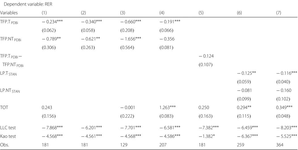
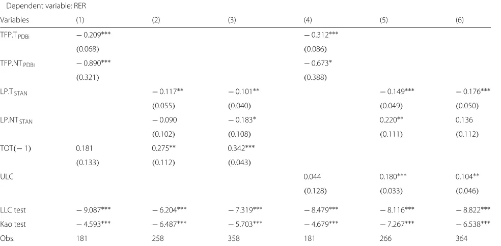
Table5summarizes the results. Compared to Table4,
the coefficients on TFP.T are smaller but are always neg-ative and statistically significant. With the terms of trade
taken into account, a 10% increase in the TFP.TPDBi
relative to the sample mean implies a 2.3% depreciation of the real exchange rate (column (1)). Indeed, omitting TOT leads to a stronger negative effect (column (2)), which is in line with the theoretical framework developed
by Benigno and Thoenissen (2003). Remarkably, though,
the negative relationship between TFP.TPDBiand the real
exchange rate persists even after including the terms of trade to control for the effects of the home bias. More-over, this result continues to hold when the number of leads and lags increases to three (column (3)) or when the method is changed to the group-mean FMOLS estimator
(column (4))29. The group-mean FMOLS estimation
fur-ther reveals that six countries (Belgium, Denmark, France, Italy, Norway, and the USA) exhibit a statistically signif-icant negative effect, while only three countries (Greece, Netherlands, and Sweden) exhibit a statistically significant
positive effect30. An opposite Balassa-Samuelson effect
still occurs if we include relative sectoral productivity as a single regressor, as shown in column (5)31.
The results are similar to the findings of Tintin (2014) from a single regression analysis. While most studies include countries with floating exchange rates, Berka et al. (2018) focus on countries in the euro area to investigate the link between real exchange rates and sectoral TFP. As a result, nominal exchange rate movements that are
Table 5The Balassa-Samuelson effect in recent times
Dependent variable: RER
Variables (1) (2) (3) (4) (5) (6) (7)
TFP.TPDBi −0.234∗∗∗ −0.340∗∗∗ −0.660∗∗∗ −0.191∗∗∗
(0.062) (0.058) (0.208) (0.066)
TFP.NTPDBi −0.789∗∗ −0.621∗∗ −1.656∗∗∗ −0.356
(0.306) (0.263) (0.564) (0.081)
TFP.TPDBi− −0.124
TFP.NTPDBi (0.107)
LP.TSTAN −0.125∗∗ −0.116∗∗∗
(0.059) (0.040)
LP.NTSTAN −0.081 −0.160
(0.099) (0.102)
TOT 0.243 −0.001 1.263∗∗∗ 0.250 0.294∗∗ 0.349∗∗∗
(0.156) (0.222) (0.083) (0.163) (0.115) (0.048)
LLC test −7.868∗∗∗ −6.201∗∗∗ −7.701∗∗∗ −6.581∗∗∗ −7.382∗∗∗ −6.459∗∗∗ −8.203∗∗∗
Kao test −4.568∗∗∗ −4.561∗∗∗ −4.568∗∗∗ −4.586∗∗∗ −1.382∗ −6.367∗∗∗ −5.525∗∗∗
Obs. 181 181 129 207 181 259 364
Notes:See Table1for the definitions of the variables. Panel DOLS estimates in (1)–(3), and in (5)–(7): all FE estimator regressions include country-specific and time-specific
likely to influence the short-run real exchange rate, and thus may weaken this link, are absent. The authors find evidence of a BS effect. We follow Berka et al. (2018) by re-estimating columns (1) and (4) using only countries in
the euro area for the sample period 1995–200832. The
results are shown in Table 8 in Appendix 2. While we
still find a negative relationship between productivity in the tradable sector and the real exchange rate, the effect decreases.
Moreover, with LP data from the STAN data set, the estimated coefficient is also negative. A 10% increase in
the LP.TSTAN implies a 1.3% depreciation of the real
exchange rate (column (6)). The extension of the time period back to 1970 hardly affects the result (column 7). Thus, both TFP data from PDBi and LP data from STAN reveal a negative relationship between productivity of tradables and RER. This contradicts the BS hypothe-sis and the earlier findings from the literature, which are
based on the ISDB data set33. However, our results are
in line with the findings of Fazio et al. (2007), who also
use LP data from STAN, and Égert et al. (2006) using
LP data from a different source. Moreover, taking labor productivity data for advanced countries from sources
other than the OECD, Ricci et al. (2013) show reversed
(but statistically insignificant) BS effects for the period 1980–2004.
Because the coefficients for LP.TSTANare similar across both samples (1984–2008 in column (6) and 1970– 2008 in column (7)), the difference from the finding in
Section 4.1cannot exclusively be explained by differing
sample periods. However, the coefficient on LP.TSTAN
for the extended estimation period has the lowest mag-nitude across all model specifications. Moreover, as
shown in column (1) of Table 9 in Appendix 2, the
re-estimation of the model with all countries available in the STAN data set leads to a still negative but sta-tistically and economically insignificant coefficient on LP.TSTAN (sample (iii), Appendix 1.1)34. Therefore, the negative relationship between the productivity of trad-ables and RER seems to have strengthened in recent
times35. The possibility of changes over time in the BS
effect has also been documented by Bordo et al. (2017)
and Bergin et al. (2006). Furthermore, this finding is
also in line with the theoretical model developed by Gubler and Sax (2014).
We include TOT in order to control for shifts in global demand and the effects of the home bias in consump-tion preferences. However, the inclusion of TOT raises concerns about possible endogeneity because TOT and the real exchange rate are endogenous relative prices and so they are simultaneously determined. First, we con-duct a very simple exercise to check for reverse causa-tion by substituting the contemporaneous value with the 1-year lagged value of TOT. Second, we replace TOT with
unit labor costs (ULC) based on the work by Berka et al.
(2018). They show in a New Keynesian model the
rela-tion between the two. The use of ULC also allows to circumvent the problem arising from the fact that one would ideally need bilateral TOT, which are not read-ily available. The estimation results with both TFP and LP data as explanatory variables are shown in Table 7 in Appendix 2. As Berka et al. (2018), we find that unit labor costs are positively related to the real exchange rate, although the magnitude is somewhat lower in our esti-mates than in the panel regressions by Berka et al. (2018). Importantly, however, the real exchange rate remains neg-atively related to productivity of tradables after these
modifications of the estimation model36. Therefore, we
conclude that conceptual and empirical difficulties with the use of TOT are not a major concern in our analysis37.
Additionally, we re-estimate the model, first, by using NFA and RI instead of TOT, and second, reducing the
country set to sample (i)38, on which the results of the
previous section are based. According to the results
dis-played in columns (2) and (3) of Table 9 in Appendix2,
these modifications do not change the conclusions about the effect of the productivity of tradables on the real exchange rate. With regard to the classification of the subsectors into tradable and non-tradable, we follow De Gregorio and Wolf (1994), who classify agricultural prod-ucts as tradables, although the agriculture subsector is highly protected in some countries. However, removing the agriculture subsector from the data set has no mean-ingful impact on our results (see column (4) of Table 9
in Appendix 2). Moreover, we follow MacDonald and
Ricci (2007) by excluding the business service subsector
from the data set because of missing observations despite of its importance for most countries. In fact, adding the business service subsector to the non-tradable sec-tor at the expense of fewer observations strengthens our
main finding (see column (5) of Table 9 in Appendix 2).
Since it is unclear whether the distribution subsector can actually be classified as non-tradable, we do not include it in our baseline estimate. In order to verify whether its inclusion changes our findings, we re-estimate the model with the distribution subsector added to the non-tradable sector. The results are displayed in columns (6) and (7) of Table 9. The coefficient on tradable TFP remains negative, albeit not statistically significant any-more (see column 6). However, replacing TFP with LP restores the statistically significant negative relationship (see column 7).
−0.2 −0.1 0.0 0.1 0.2 −0.2 −0.1 0.0 0.1 0.2 Bivariate Plot
Tradable Total Factor Productivity
Real Exchange Rate
AUT95 AUT96 AUT97 AUT98AUT99 AUT00 AUT01 AUT02 AUT03 AUT04 AUT05AUT06AUT07
AUT08 BEL95 BEL96 BEL97BEL98 BEL99 BEL00 BEL01BEL02 BEL03 BEL04 BEL05 BEL06 BEL07 BEL08 DEU94 DEU95 DEU96 DEU97 DEU98 DEU99
DEU00DEU03DEU05DEU02DEU04DEU01DEU07DEU06 DEU08 DNK96DNK97 DNK98 DNK99 DNK00 DNK01 DNK02DNK03 DNK04 DNK05DNK06 ESP00 ESP01 ESP02 ESP03 ESP04 ESP05 ESP06 ESP07 FIN84 FIN85 FIN86 FIN87 FIN88 FIN89FIN90 FIN91 FIN92 FIN93 FIN94 FIN95 FIN96FIN97 FIN98FIN99FIN00FIN01
FIN02FIN03FIN04 FIN05FIN06FIN08FIN07 FRA84 FRA85 FRA86 FRA87 FRA88 FRA89 FRA90 FRA91 FRA92 FRA93 FRA94 FRA95FRA96 FRA97FRA98 FRA99 FRA00 FRA01FRA03FRA02 FRA04 FRA05 FRA06 GRC98 GRC99 GRC00GRC01 GRC02 GRC03 GRC04GRC05 GRC06GRC07GRC08
ITA84ITA85 ITA86ITA87ITA88ITA89 ITA90 ITA91 ITA92 ITA93 ITA94 ITA95 ITA96 ITA97 ITA98 ITA99 ITA00 ITA01 ITA02 ITA03 ITA04 ITA05 ITA06 ITA07 ITA08 NLD95 NLD96 NLD97NLD99NLD98 NLD00 NLD01NLD02 NLD03NLD04NLD05NLD06NLD07 NLD08 NOR84 NOR85 NOR86NOR87 NOR88 NOR89 NOR90 NOR91 NOR92 NOR93 NOR94 NOR95 NOR96 NOR97 NOR98 NOR99 NOR00NOR01 NOR02 NOR03 NOR04 NOR05 NOR06 NOR07 SWE96 SWE97 SWE98SWE99SWE00
SWE01SWE02 SWE03SWE04
SWE05SWE07SWE06 USA84 USA86 USA87 USA88 USA89 USA90 USA91 USA92 USA93 USA94 USA95 USA96 USA97 USA98 USA99 USA00 USA01 USA02 USA03
USA04USA06USA05
USA07
−0.2 −0.1 0.0 0.1 0.2
−0.2
−0.1
0.0
0.1
0.2
Partial Regression Plot
Tradable Total Factor Productivity Residuals
Real Exchange Rate Residuals
AUT95 AUT96 AUT97 AUT98 AUT99 AUT00AUT01 AUT02 AUT03 AUT04 AUT05AUT06AUT07
AUT08 BEL95 BEL96 BEL97BEL98 BEL99 BEL00 BEL01 BEL02 BEL03 BEL04 BEL05 BEL06 BEL07 BEL08 DEU94 DEU95 DEU96 DEU97 DEU98 DEU99 DEU00DEU01 DEU02 DEU03DEU04 DEU05DEU07DEU06
DEU08 DNK96 DNK97 DNK98 DNK99 DNK00DNK01 DNK02DNK03 DNK04 DNK05DNK06 ESP00 ESP01 ESP02 ESP03 ESP04 ESP05 ESP06 ESP07 FIN84 FIN85FIN86 FIN87 FIN88 FIN89 FIN90 FIN91 FIN92 FIN93 FIN94 FIN95 FIN96FIN97FIN98FIN99FIN00FIN01
FIN02 FIN03 FIN04FIN05FIN06FIN07FIN08
FRA84 FRA85 FRA86 FRA87 FRA88 FRA89 FRA90 FRA91 FRA92 FRA93 FRA94 FRA95FRA96
FRA97FRA01FRA00FRA98FRA99 FRA02 FRA03 FRA04 FRA05 FRA06 GRC98 GRC99 GRC00 GRC01 GRC02 GRC03GRC04 GRC05 GRC06 GRC07 GRC08 ITA84 ITA85
ITA86ITA87ITA89ITA88 ITA90ITA92ITA91
ITA93 ITA94 ITA95 ITA96 ITA97 ITA98 ITA99 ITA00 ITA01 ITA02 ITA03 ITA04 ITA05 ITA06 ITA07 ITA08 NLD95 NLD96 NLD97NLD98 NLD99 NLD00NLD01NLD02 NLD03NLD04NLD06NLD05 NLD07 NLD08 NOR84 NOR85 NOR86 NOR87 NOR88 NOR89 NOR90NOR91 NOR92NOR93 NOR94 NOR95 NOR96 NOR97 NOR98 NOR99 NOR00 NOR01 NOR02 NOR03 NOR04NOR05 NOR06 NOR07 SWE96 SWE97 SWE98SWE99 SWE00 SWE01SWE02 SWE03SWE04
SWE05SWE06SWE07 USA84USA85 USA86 USA87 USA88 USA89 USA90 USA91USA92 USA93 USA94 USA95 USA96 USA97USA98 USA99 USA00 USA01 USA02 USA03 USA04USA05 USA06 USA07
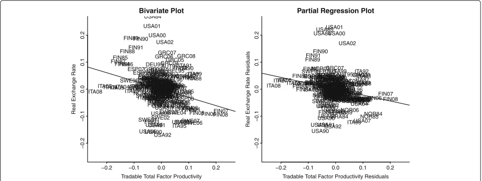
Fig. 1Tradable productivity and the real exchange rate: using data from 1984 to 2008, the plots show the relationship between the real exchange rate and total factor productivity from the OECD productivity database (PDBi). The plots on the left side show the bivariate relationship of the two variables (both the productivity measure and the real exchange rate have been adjusted by country and time fixed effects). The plots on the right side show the results of partial regressions (Velleman and Welsch1981). On the vertical axis, they show the residuals of a regression of the real exchange rate on the following control variables: non-tradable productivity, terms of trade, country, and time fixed effects. On the horizontal axis, they show the residuals of a regression of productivity in the tradable sector based on the same control variables
and Welsch1981): the residuals of a regression of the real exchange rate on two additional control variables (non-tradable productivity, terms of trade) in addition to the fixed effects (vertical axis) are plotted against the residu-als of a regression of productivity in the tradable sector on the same four control variables (horizontal axis). The small differences between the left and the right panel indi-cate that the relationship does not depend on whether control variables are used. In line with the estimation results, the scatter plots show the significant negative relationship.
Again, the effect of non-tradable productivity on RER is less robust. The findings mostly confirm the BS hypoth-esis, although in two estimations, the coefficient on the productivity in the non-tradable sector switches its sign
(columns (1) and (3) of Table 9 in Appendix 2). The
group-mean FMOLS estimate (column (4) of Table 5)
identifies four countries with a significant negative
rela-tionship between TFP.NTPDBi and RER and five
coun-tries with a significant positive relationship between
TFP.NTPDBi and RER40. Therefore, the relationship
between non-tradable productivity and the real exchange rate seem to differ across the countries, making a within-dimension panel approach for analyzing this relationship questionable.
Our findings suggest that terms of trade are a key driver of the real exchange rate, which confirms ear-lier results (see, e.g., (De Gregorio and Wolf1994) for a
panel of OECD countries or (Sax and Weder 2009) and
(Mancini Griffoli et al. 2015) for Switzerland). TOT is
statistically and economically significant with the correct
sign in columns (4)–(6) of Table 5 as well as columns
(1), (3), and (7) of Table 9 in Appendix 2. On
aver-age, a 10% increase in the terms of trade leads to an appreciation of the real exchange rate of approximately 3%. Next, we examine the impact of additional explana-tory variables on the long-run real exchange rate and on the reversed BS effect of productivity in the tradable sector.
4.3 The impact of additional control variables
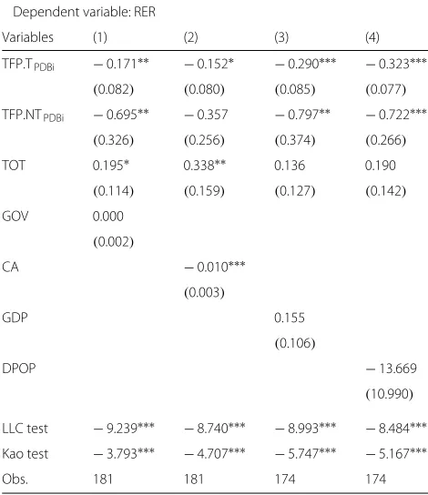
The impact of additional explanatory variables on the
long-run real exchange rate is analyzed in Table 6. In
line with the results in Section4.2, both coefficients on the productivity variables are negative and predominantly significant in all models. For the tradable sector pro-ductivity, this is the opposite effect of what is claimed by the BS hypothesis. Additionally, the significant pos-itive impact of the terms of trade on the price level remains.
The selection of the explanatory variables is discussed in
Section2.3. Government spending (GOV) has no
Table 6The impact of additional control variables
Dependent variable: RER
Variables (1) (2) (3) (4)
TFP.TPDBi −0.171∗∗ −0.152∗ −0.290∗∗∗ −0.323∗∗∗ (0.082) (0.080) (0.085) (0.077) TFP.NTPDBi −0.695∗∗ −0.357 −0.797∗∗ −0.722∗∗∗
(0.326) (0.256) (0.374) (0.266)
TOT 0.195∗ 0.338∗∗ 0.136 0.190
(0.114) (0.159) (0.127) (0.142)
GOV 0.000
(0.002)
CA −0.010∗∗∗
(0.003)
GDP 0.155
(0.106)
DPOP −13.669
(10.990)
LLC test −9.239∗∗∗ −8.740∗∗∗ −8.993∗∗∗ −8.484∗∗∗
Kao test −3.793∗∗∗ −4.707∗∗∗ −5.747∗∗∗ −5.167∗∗∗
Obs. 181 181 174 174
Notes:See Table1for the definitions of the variables. Panel DOLS estimates in (1)–(4):
all FE estimator regressions include country-specific and time-specific dummy variables as well as first differences of each explanatory variable (1 lead/lag). Sample period 1984-2008. Country sample (Appendix1.1): sample (ii). The productivity data stem from the PDBi. Robust standard errors proposed by Driscoll and Kraay (1998) are reported in parentheses. LLC test: Cointegration test following MacDonald and Ricci (2007):tstatistic of Levin et al. (2002) (lag length selection by SIC; Bartlett kernel, Newey-West bandwidth). Kao test: cointegration test proposed by Kao (1999):t
statistic (lag length selection by SIC; Bartlett kernel, Newey-West bandwidth). *, **, and *** denote significance at the 10%, 5%, and 1% levels, respectivel
affects RER positively (column (3))—a 10% increase in GDP implies a 1.6% appreciation of the real exchange rate—but the effect is not statistically significant. Finally, contrary to the theory, in our sample of OECD countries, there is no significant connection between the population growth rate (DPOP) and RER (column (4)). Therefore, of all the additional explanatory variables, it is only the terms of trade that are fairly robust against a sample variation.
5 Summary and conclusions
This paper explores the robustness of the Balassa-Samuelson (BS) hypothesis. We analyze a panel of OECD countries from 1970 to 2008 and compare three different data sets on sectoral productivity provided by the OECD, including a newly constructed data set on total factor productivity (TFP).
Overall, we cannot find support for the BS hypothesis. In contrast, our within-dimension DOLS and between-dimension FMOLS estimations point to a robust nega-tive equilibrium relationship between productivity in the
tradable sector and the real exchange rate for the time since the mid-1980s. We find this negative relationship with respect to TFP from the new Productivity Database (PDBi) as well as with sectoral labor productivity (LP)
from the STAN data set (see also Égert et al. (2006) and
Fazio et al. (2007)). The results from estimations with LP indicate that the negative effect of tradable productivity on the real exchange rate has strengthened over time. The finding not only contradicts the BS hypothesis but also the results of previous empirical research that is based on the older International Sectoral Database (ISDB). Our anal-ysis suggests that the choice of the model specifications matters for the finding as to whether the empirical rela-tionship between the productivity of tradables and the real exchange rate is negative or positive for the time period from 1970 to 1992, using the ISDB.
An extensive robustness analysis shows that the neg-ative relationship does not depend on the choice of the productivity measure, the choice of the country sam-ple, the precise start of the time period, the exact model specification, and the inclusion of additional explanatory variables. This result holds even after including the terms of trade to control for the effects of the home bias. On the other hand, the relationship between productivity in the non-tradable sector and the long-run real exchange rate for the time since 1984 is affected by the choice of the country sample. Prior to 1992, the robustness tests reveal a strong dependency of the results on a single outlier: the coefficient on non-tradable labor productivity signif-icantly changes the sign once Japan is included. Without Japan, we find a robust negative relationship between non-tradable productivity and the real exchange rate, in line with the BS hypothesis.
Finally, we examine the explanatory power of control variables, whose importance for the real exchange rate determination has been discussed in the literature. The results indicate that, with the exception of the terms of trade, their explanatory power is weak or not robust against the chosen time period.
The fact that we find a robust negative relationship between tradable productivity and the real exchange rate is puzzling. According to the Balassa-Samuelson hypothesis, we would expect higher productivity to be connected with higher wages and thus with a higher price level.
Based on these findings, we conclude that the the-oretical framework leading to the Balassa-Samuelson hypothesis needs to be modified to be in line with the empirical data. The literature has proposed the home bias in consumption preferences, as a possible modification: a rise in tradable productivity lowers the price of its goods relative to those abroad. This may offset the increase of the relative price of non-traded goods (see, e.g., Benigno and
and Schembri (2010) or Berka et al. (2018)). However, we find a significant negative relationship between the
productivity of tradables and the real exchange rate
despite controlling for the impact of movements in exports relative to import prices on the real exchange rate. This result suggests that a rise in productiv-ity in the tradable sector can lead to a decrease in the relative price of non-traded goods. Gubler and
Sax (2014) develop a static general-equilibrium
frame-work with skill-based technological change (SBTC), in which a productivity increase in the tradable sector can lower the wages of low-skilled workers, which in turn leads to lower prices of non-tradables and thus to a depreciation of the real exchange rate.
Endnotes
1Rogoff (1996) shows that the speed of adjustment of
real exchange rates is too slow to be in line with the PPP theory. Recent studies challenge this finding and stress
the importance of non-linear adjustments (Taylor2003)
or dynamic aggregation bias (Imbs et al.2005). Altogether, the empirical evidence for PPP is mixed (for reviews, see
Froot and Rogoff (1996); Taylor (2003) or Gengenbach
et al. (2009)
2Égert et al. (2006) provide an extensive survey with a
focus on transition economies.
3However, we also find the results in favor of the BS
hypothesis with data from the ISDB.
4While Fazio et al. (2007) also use a panel DOLS
frame-work, we also employ a between-dimension group-mean panel FMOLS estimator.
5Lee and Tang (2007) and Ricci et al. (2013) also find a
negative, though not statistically significant, relationship between productivity of tradables and the real exchange rate. While the result of the former is based on TFP for OECD countries from the ISDB, that of the latter is based on LP calculated using several data sources for a broad range of advanced economies. Focusing on Switzerland, Sax and Weder (2009) and Mancini Griffoli et al. (2015) conclude that changes in sectoral LP do not play a signifi-cant role in explaining real exchange rate movements.
6For empirical evidence for deviations from the law of
one price see, e.g., Engel (1999).
7MacDonald and Ricci (2007) and Choudhri and
Schembri (2010) provide further results on this
mecha-nism. In contrast, higher productivity in the traded goods sector results in terms of trade improvements and ampli-fies the Balassa-Samuelson effect in the model developed by Corsetti et al. (2008).
8There is no “pricing-to-market” by sellers in their
model, and they consider a single currency area.
9In the small economy model developed by
Devereux (1999), the real exchange rate depreciates
because endogenous productivity gains in the service sector lead to a fall in traded goods prices that off-sets the BS effect. However, because we exclude the distribution subsector due to classification difficulties
(MacDonald and Ricci 2005), this seems not to be the
main mechanism that explains the potentially negative relationship between rising productivity in the tradable sector and the real exchange rate in our study. More recently, Bordo et al. (2017) emphasize that the impact of productivity on the real exchange rate varies over time due to changes in trade costs that affect the terms of trade.
10All country samples featured in our estimations are
presented in Appendix1.1
11In order to verify this claim, we estimate our baseline
model with a reference country for each variable. We then re-estimate the same model without using a reference country and obtain identical coefficients and standard errors for all but time fixed effects.
12Nonetheless, our main results are robust against the
inclusion of the effective real exchange rate (source: OECD Economic Outlook, competitiveness indicator) instead of the unweighted real exchange rate, RER (results not shown).
13Note that there are methodological differences
compared to the calculated sectoral TFP data in the KLEMS database. For example, whereas in the EU-KLEMS database sectoral TFP is affected by changes in the composition of labor and capital over time, this is not the case for the sectoral TFP data from
PDBi used in this paper (Arnaud et al. 2011).
How-ever, Arnaud et al. (2011) compare the average TFP
change from 1990 to 2007 in manufacturing and services of 13 countries. While average TFP growth is substan-tially higher in PDBi/STAN compared to EU-KLEMS, the relative TFP growth rates in manufacturing between countries are very similar (except for Ireland, which is excluded in our study), which mainly determines our main finding.
14In a robustness analysis, we remove the agriculture
15Adjustments of the threshold value to 5% and 20%
leave the division virtually unchanged (De Gregorio and Wolf1994).
16In a robustness analysis, we add the business service
subsector to the non-tradable sector at the expense of fewer observations because of its importance for most countries.
17In a robustness analysis, we add the distribution
sub-sector to the non-tradable sub-sector.
18The advantages are summarized by Canzoneri
et al. 1999: first, the labor productivity data are avail-able for more countries and over a longer time period than the TFP numbers. Second, the calculation of LP figures does not require an estimation of the capital stock and the income share of labor, with both esti-mations likely to be imprecise. Third, the BS hypothe-sis holds for more technologies than the Cobb-Douglas production function, which is generally employed to determine TFP.
19This reflects the use of time-specific dummy
vari-ables in all panel estimations. For a brief discussion on the effects of the use of time-specific dummy variables for the choice of the reference country see Section2.1.
20Non-stationarity of productivity is also consistent
with theoretical macroeconomic models (see, e.g., King et al. (1991); Galí (1999) or Lindé (2009)).
21The leads and lags remove the correlation between
the error term and the stationary component of the non-stationary variables.
22As a robustness check, we employ the HC3 estimator
proposed by Long and Ervin (2000). The conclusions do
not change.
23For the theoretical foundation of this methodology,
see Pedroni (2004). The conclusions do not change if the
residuals are corrected by the estimated leads and lags.
24Because of the limited number of observations for
every country, we prefer the FMOLS estimator to the DOLS estimator for the group-mean estimations.
25To capture the short-run dynamic adjustment of
the real exchange rate to temporary disequilibria, an error correction specification is applied to the data. The estimated half-life of deviations of the real exchange rate from its estimated long-run relationship of approx-imately one to three and a half years, depending on the model specification, is in line with the existing literature.
26Notice that due to the lack of data for some years, the
coverage is not exactly the same. For the period from 1970 to 2008, Sweden is not covered by the STAN data set. See
Figure 2 in Appendix1for more details.
27We exclude Canada from the sample since there are
missing data for Canada from 2004 onwards, which does not affect the conclusions.
28Notice that due to the lack of data for some years,
the coverage is not exactly the same. See Figure 2 in
Appendix1for more details.
29We also repeatedly re-estimate this specification and
each time omit one of the countries. This exclusion exer-cise reveals that the negative sign is persistent against the omission of any country. In rare cases, the coefficient becomes statistically insignificant.
30For the remaining three countries, TFP.T
PDBiis twice insignificantly negative (Austria and Germany) and only once insignificantly positive (Finland).
31We repeat this exercise using LP instead of TFP
and find a negative coefficient of similar magnitude (−0.129) on relative sectoral productivity. In this specifi-cation, the coefficient is statistically significant at the 10% level.
32This is comparable to the countries and years
consid-ered by Berka et al. (2018) (see Table 4 of their study). Our sample period ends in 2008 instead of 2009. Moreover, we do not have data on Ireland; for Spain, we only have a small sample size.
33One exception is the study by Lee and Tang (2007).
The authors use sectoral TFP data from ISDB and find a negative, though not statistically significant, relationship between productivity of tradables and the real exchange rate in their baseline estimation.
34As described in Section2.2, agriculture,
manufactur-ing, and transport, storage, and communications are clas-sified as tradables. If we assume that only manufacturing constitutes the tradable sector, neglecting the other two subsectors, the negative effect is still statistically signifi-cant but remains economically small. Focusing on man-ufacturing might be appropriate since its classification as tradable is the least controversial.
35Varying the start point of the estimation sample