Real-time rendering of aerial perspective effect based on turbidity estimation

R E S E A R C H P A P E R

Open Access

Real-time rendering of aerial perspective

effect based on turbidity estimation

Carlos Morales

, Takeshi Oishi

and Katsushi Ikeuchi

Abstract

In real outdoor scenes, objects distant from the observer suffer from a natural effect called aerial perspective that fades the colors of the objects and blends them to the environmental light color. The aerial perspective can be modeled using a physics-based approach; however, handling with the changing and unpredictable environmental illumination as well as the weather conditions of real scenes is challenging in terms of visual coherence and computational cost. In those cases, even state-of-the-art models fail to generate realistic synthesized aerial perspective effects. To overcome this limitation, we propose a real-time, turbidity-based, full-spectrum aerial

perspective rendering approach. First, we estimate the atmospheric turbidity by matching luminance distributions of a captured sky image to sky models. The obtained turbidity is then employed for aerial perspective rendering using an improved scattering model. We performed a set of experiments to evaluate the scattering model and the aerial perspective model. We also provide a framework for real-time aerial perspective rendering. The results confirm that the proposed approach synthesizes realistic aerial perspective effects with low computational cost, outperforming state-of-the-art aerial perspective rendering methods for real scenes.

Keywords: Real-time rendering, Aerial perspective, Shader programming

1 Introduction

In real open-air scenes, when a target object viewed by an observer is far, the perceived object’s appearance changes, being fainted and blended to the environmental light color. This natural effect is known asaerial perspective

and is due to the light scattering by particles suspended in the atmosphere.

The importance of aerial perspective rendering is reflected in several applications, as illustrated in Fig. 1. It can be employed in image and video composition to generate artistic atmospheric effects over real scenes. It can also be used in computer vision (CV) and com-puter graphics (CG) for rendering virtual objects with an appearance according to the outdoor scene. Namely, fields such as mixed reality (MR), where CG models are merged into a real scene, can exploit aerial perspective rendering to output more realistic virtual objects.

In general, we have to render an artificial aerial per-spective effect on a target object to emulate the natural

*Correspondence: [email protected] 1_{The University of Tokyo, Tokyo, Japan}

Full list of author information is available at the end of the article

atmospheric effect. This goal is specially more difficult in real-time applications in outdoor scenes, which present a challenge due to the variant illumination and atmospheric conditions such as clear, hazy, or cloudy days.

A conventional approach for aerial perspective render-ing is to find an outdoor light scatterrender-ing model with parameters that lead to generate a realistic synthesized look according to the real scene. Such scattering mod-els can be analyzed from captured skies using sky illu-mination models [1–7]. Due to its simplicity and accu-racy for scattering modeling, a heuristic parameter called

turbidity (T) has been used to categorize atmospheric conditions [8–12]. Following that approach, we propose a full-spectrum turbidity-based aerial perspective model that enables us to render realistic aerial perspective effects in real time. Our model heavily relies on estimating tur-bidity from clear-sky regions of a captured omnidirec-tional sky image. Thus, scenes where the sky is not visible are beyond the scope of this work.

Method overview: The overview of our aerial perspec-tive rendering approach is illustrated in Fig. 2. Input data is a real omnidirectional sky image captured by fisheye lens camera and theinput scene, which can be captured by

Fig. 1Aerial perspective rendering with our method.Top row: An input image and the re-targeted synthesized aerial perspective effect (from left to right).Bottom row: A MR application before and after aerial perspective rendering

the same camera or a different perspective or panoramic camera. In image and video composition applications, the input scene is represented by its RGB intensity color, its depth map, and the spectral sensitivity of the camera used to capture the input scene. In MR applications, the input scene is composed of the RGB intensity color of the real scene, the color and depth of the virtual object, and the camera’s spectral sensitivity. The problem addressed in this paper is to estimate the turbidity from the omnidirec-tional sky image and then use it to render an aerial per-spective effect. While the aerial perper-spective is rendered over the de-hazed input scene in composition applica-tions, it is rendered only on the virtual object in MR. For this purpose, our method consists of the following stages:

1) Turbidity estimation: The captured omnidirectional sky image is compared with turbidity-based sky models to find the turbidity value that provides the best matching (Section 3.4).

2) Aerial perspective rendering: An improved turbidity-based scattering model (Section 5) is used in a

full-spectrum aerial perspective rendering equation (Section 4) to generate the finalsynthesized scene. This stage is performed in real time in a graphics processing unit (GPU) framework (Section 6).

Contributions: The main contributions of this work are threefold:

1) Improved turbidity-based scattering model for rendering that fit to real atmospheric effects more accurately than previous works [3, 13].

2) A novel full-spectrum, turbidity-based aerial perspective rendering model that synthesizes plausible aerial perspective effects in real scenes and improves over previous works [13–15] in terms of visual coherence.

3) A real-time framework for aerial perspective effect rendering. The implementation delivers more than two orders of magnitude speed-up compared to prior art [13], allowing real-time performance needed in applications such as MR.

2 Related work

Previous methods for aerial perspective modeling and rendering rely on understanding the scattering phenom-ena in the atmosphere. McCartney [16] presented an excellent review of former works on atmospheric optics. His work contains relevant data about the scattering phe-nomena under different weather conditions categorized by the heuristic parameter turbidity (T). T is used to model the scattering by molecules of air and larger parti-cles, such as haze, and is employed for classifying various atmospheric conditions ranging from pure air to fog. Since the atmospheric phenomenon in [16] is modeled using real data, it has been used in both CV and CG fields. However, such models have been used differently, varying depending on whether the aim is oriented to CV or CG.

2.1 CG-oriented aerial perspective rendering

In this category, the atmospheric optics models are tar-geted for completely virtual scenes. Preetham et al. [3] presented a full-spectrum turbidity-based analytical sky model for various atmospheric conditions. Based on that model, they developed an approximated scattering model for aerial perspective rendering. Dobashi et al. [17] intro-duced a fast rendering method to generate various atmo-spheric scattering effects via graphics hardware. Nielsen [18] presented a real-time rendering system for simu-lating atmospheric effects. Riley et al. [19] presented a lighting model for rendering several optical phenomena. Schafhitzel et al. [20] rendered planets with atmospheric scattering effects in real time. Bruneton and Neyret [5] rendered both sky and aerial perspective from all view-points from the ground to outer space.

The synthesized atmospheric effects generated by the mentioned works are visually plausible in fully CG scenes where the illumination is controlled. However, their direct implementation in real scenes does not have a similar per-formance, since the scattering models need to be tuned to fit the variant, natural outdoor illumination. Moreover, such models are usually targeted as post processing effects where visual quality is more important than computa-tional cost.

2.2 CV-oriented aerial perspective rendering

This group of methods model the atmospheric phe-nomenon in real outdoor scenes. Using scattering models, several works were able to restore captured images at different weather conditions. Gao et al. [21] presented an aerial perspective model for haze filtering based on a parameter called maximum visibility. Zhu et al. [15] developed a linear color attenuation prior for image de-hazing based on a parameter calledscattering coefficient. The synthesized results from these works successfully cor-rected and restored at some extent the color of images under hazy conditions. However, these methods are not

automatic and the results depend on manual tuning of either the maximum visibility in [21] or the scattering coefficient in [15], which control the amount of de-hazing. Automatic image restoration approaches have also been proposed in the literature. Narasimhan and Nayar [22] proposed a physics-based scattering model to describe the appearances of real scenes under uniform bad weather conditions. Using that scattering model, their method restored the contrast of one image; nonetheless, their method required a second image of the same scene under a different weather condition. This limitation was over-come by He et al. [14], who proposed an automatic haze-removal approach for single images using a dark channel as prior. Results in [14] showed consistent and fast image de-hazing. However, using their method for aerial perspective rendering leads to appearances that are incon-sistent with natural aerial perspective, especially in cases with high haze densities.

To solve the previous drawbacks, Zhao [13] proposed an automatic turbidity-based aerial perspective model. In his approach, turbidity was estimated from captured omnidi-rectional sky images. The camera’s spectral sensitivity was estimated for conversion from spectral radiance to RGB pixel values. Combining the estimated spectral sensitiv-ity and a simple correction of Preetham’s scattering model [3], his method was able to generate an aerial perspective effect over virtual objects for outdoor MR. However, his method makes the appearance of the synthesized virtual object suffer from a strong aerial perspective effect even for low turbidity values at short distances. Moreover, his approach has a high computational cost.

3 Preliminary

3.1 Aerial perspective modeling

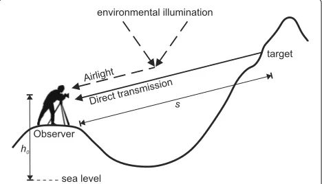
Figure 3 illustrates a general model of aerial perspective. The total light perceived by the observer is a summa-tion of two components:direct transmissionandairlight. The direct transmission stands for the light that comes

from the target following the optical path and is atten-uated until it reaches the observer. The airlight is the environmental light that is scattered in the same direction as the direct transmission and then is attenuated in the way to the observer. The aerial perspective under various atmospheric conditions is broadly modeled as [22–24]:

L(s,λ) = L(0,λ)e−βsc(λ)s

+L(∞,λ)

1−e−βsc(λ)s

, (1)

whereL(s,λ)is the total light perceived by the observer,

L(0,λ)is the light coming from the target without aerial perspective effect, andL(∞,λ) is the atmospheric light.

s is the distance between the target and the observer, andλis the light wavelength.βscis the total atmospheric scattering coefficient modeled as

βsc=βR+βM, (2) where βR is the Rayleigh scattering coefficient that ana-lyzes particles much smaller thanλ, such as molecules of air, andβM is the Mie scattering coefficient that models particles whose size is nearly equal toλ, such as particles of haze.

The Rayleigh scattering coefficient is given by [25]

βR=

8π3(n2−1)2 3Nλ4

6+3pn

6−7pn

e−Hh_{R0, (3)}

and the Mie scattering coefficient is expressed by [26]

βM=0.434c(T)π

2π

λ

ν−2

K(λ)e−

h

H_{M0, (4)}

wheren= 1.0003 is the refractive index of air in the vis-ible spectrum,N = 2.545×1025 m−3is the molecular number density of the standard atmosphere,pn = 0.035

is the depolarization factor for air,his the altitude at the scattering point,HR0 =7994 m is the scale height for the Rayleigh scattering,c(T)is the concentration factor that depends on the atmospheric turbidity,ν=4 is the Junge’s exponent,K(λ)is the wavelength-dependent fudge factor, andHM0=1200 m is the scale height for Mie scattering.

3.2 Atmospheric condition via turbidity

Turbidity is defined as the ratio of the optical thickness of the atmosphere composed by molecules of air plus larger particles to the optical thickness of air molecules alone [16]:

T=

hf

hiβR(h)dh+

hf

hiβM(h)dh

hf

hiβR(h)dh

, (5)

where hi andhf are the initial and final altitudes of the optical path, respectively.

Preetham et al. [3] presented an analytical sky model for various atmospheric conditions through turbidity. Their model relates the luminance Y(cd/m2) of sky in any

viewing directionV with respect to the luminance at a reference pointYzby

Y= F(θ,γ,T) F(0,θs,T)

Yz, (6)

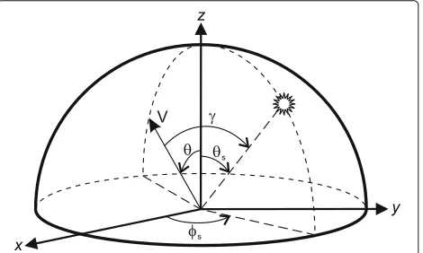
whereFis the sky luminance distribution model of Perez et al. [27], θ is the zenith angle of viewing direction, θs is the zenith angle of the sun, and γ is the angle of the sun direction with respect to the viewing direction (see coordinates in Fig. 4).

3.3 Rendering equation

In MR applications, we need an equation to convert radio-metric formulas, such as the spectral radiance, to pixel color values, such as RGB. In general, when an object is illuminated by a source of light, the reflected light goes through the camera lens and is recorded by its charged couple device (CCD). Then the recorded image intensity for the channel c∈{r,g,b} can be modeled as

Ic=

780 nm

380 nm

L(λ)qc(λ)dλ, (7)

whereL(λ)is the reflected spectral radiance at the object surface, the range 380 to 780 nm stands for the visible spectrum of light, andqc(λ)is the spectral sensitivity of the camera.

The camera’s spectral sensitivity is important for color correction since it compensates the effects of the record-ing illumination. In this matter, we benefited from Kawakami et al. [28] and the public data of spectral sensi-tivity for various cameras [29]. They estimatedqc(λ)from omnidirectional captured sky images and turbidity-based sky spectra.

3.4 Atmospheric turbidity estimation

The atmospheric turbidity can be estimated by matching the luminance distribution of turbidity-based Preetham sky models and an omnidirectional sky image captured by

a fisheye lens camera as in [13]. First, the sun position is estimated at the captured sky image by either find-ing the center of the saturated area of the sun or usfind-ing the longitude, latitude, date, and time at the observer’s position. Then the luminance ratioYi/Yref (Y from the XYZ color space) is calculated between a sampling point

iand a reference point ref that can be the zenith or any other visible point in the captured sky image. The ratio

Yi(T)/Yref(T) is computed at the corresponding points in the Preetham sky models with the same sun position using Eq. (6). The turbidity-based sky model that best matches the captured sky image is the one with the low-est difference between both ratios. Therefore, the targeted turbidity is the solution to the minimization problem:

arg min

T∈[1,20]

N

n=1

Yi(T)

Yref(T)−

Yi

Yref

, (8)

whereNis the number of sample points used in the cal-culation process. In this paper, we solve for the turbidity using the Levenberg-Marquardt algorithm (LMA), a sim-pler yet efficient approach compared to the particle swarm optimization used in [13].

Since the Preetham sky model does not provide equations for calculating the brightness of cloudy pixels, the Random Sample Consensus (RANSAC) approach is used to remove cloudy pixels (outliers) from the sampling and estimate turbidity only from clear-sky pixels (inliers).

4 Aerial perspective rendering equation

In order to render an aerial perspective effect in applica-tions that contain only real scenes or both real and virtual objects, the RGB color system is more convenient to use than a spectral radiance system. Originally, the aerial per-spective rendering equation for one viewing direction can be obtained by replacing the aerial perspective model of Eq. (1) in Eq. (7). From these equations, the observer per-ceives the intensity value Ic of a target object’s pixel at distancesfor the channel c∈{r,g,b} as

Ic =

L(0,λ)e−βsc(λ,T,h0)sqc(λ)dλ

+

L(∞,λ)1−e−βsc(λ,T,h0)sqc(λ)dλ, (9)

whereL(0,λ),L(∞,λ),βsc(·), andsare same as in Eq. (1) andh0is the altitude at the observer position.

To simplify Eq. (9) into an RGB-based rendering equation, we can assumeqc(λ)to be a narrow band. In this way, we approximated the spectral sensitivity in the direct transmission and airlight by Dirac’s delta function. Gen-eralizing this approximation for any observer’s viewing directionV(θ,φ), we obtain

Ic(s,V)=Ic0(V) c(T,s)+Ic∞(T,V) (1− c(T,s)), (10)

whereI0

cis the intensity value of a pixel at the target object, at distances, and viewing directionV, without any aerial perspective effect.I_c∞is the sky intensity value at an infi-nite distance in the same viewing directionV, and c is the attenuation factor approximated as

c(T,s)=

780 nm

380 nme−βsc(λ,T,h0)sqc(λ)dλ

780 nm

380 nmqc(λ)dλ

. (11)

In real daylight scenes, we can calculate I_c∞(T,V)

from another viewing directionV(θ,φ), with the same azimuth φ but different zenith θ, of the captured sky. First, the visible sky is roughly segmented from the textureless area of the captured image using a water-shed algorithm. Then, ahorizon regionwithin the visible sky pixels with the highest azimuth angles is estimated. Finally, I_c∞(·) is computed from pixels in the horizon region that have the highest intensity valueI_c∞(θ)by

I_c∞(T,θ)=I_c∞(θ)ς(T,θ,θ), (12)

where ς(·) is an intensity ratio modeled according to Preetham sky models as

ς(T,θ,θ)= 1+(0.178T−1.463)e

(−0.355T+0.427)/cosθ

1+(0.178T−1.463)e(−0.355T+0.427)/cosθ. (13)

5 Improved scattering model for rendering

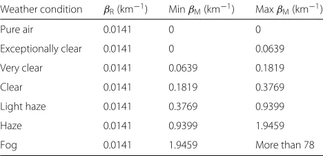
Scattering models for real scenes require parameters that guarantee a realistic result when rendering the aerial per-spective effect. For this purpose, we propose an improved scattering model based on real data of [16] about weather conditions via scattering coefficients, which is summa-rized in Table 2 of the Appendix. The data in [16] was measured under standard conditions, which is using a spectrally weighted average wavelength (λ=550 nm) for daylight within the visual spectrum at sea level (h=0 m).

5.1 Rayleigh scattering coefficient correction

We can obtain the value of the Rayleigh scattering coef-ficient ofβR = 0.0141 km−1 under standard conditions from Table 2 in the Appendix. However, using Eq. (3) for such conditions results inβR = 0.0135 km−1. This slight variation inβRof 0.0006 km−1is actually considerable in terms of the attenuation factor. According to the Inter-national Visibility Code summed up in [16], the visibility range in pure air is up to 277 km. This means that a vari-ation of 0.0006 km−1in the scattering coefficient in that visibility range affects the attenuation factor in 84.69%. To adjust this disparity, we propose a straightforward multiplicative correction factorKRgiven by

Then our modified Rayleigh scattering coefficient is given by

ˆ

βR=

8π3(n2−1)2 3Nλ4

6+3pn

6−7pn

e−

h₀ H_R0 ×_K

R, (15)

wheren,N,pn, andHR0are the same as in Eq. (3),h0is the altitude at the observer, andKRis given by Eq. (14).

5.2 Mie scattering coefficient correction

One issue in Preetham’s scattering model [3] is related to the turbidity itself. From Eq. (5),T =1 refers to the ideal case where the Mie scattering coefficient is zero. Thus, the concentration factorc = (0.6544T −0.6510)×10−16of Preetham [3] andc=(0.6544T−0.6510)×10−18of Zhao [13] should be zero forT =1. We corrected this issue to ensure a more reliable fitting to the real data in [16] by

ˆ

c(T)=(0.65T−0.65)×10−16. (16)

Another issue is the value of the fudge factorKin [3, 13]. The fudge factor affects exponentially to the part of the attenuation factor corresponding to the Mie scattering. Thus, adjusting K to the real data in [16] is essential to handle hazy atmospheric conditions accurately. Preetham et al. [3] and Zhao [13] used a wavelength-dependentK∈

[0.65, 0.69] for wavelengths λ ∈[380, 780] nm. However, such fudge factor values do not match the data in [16]. Therefore, we correctedKaccording to Table 2, calculat-ing an average fudge factor solvcalculat-ing Eq. (4) under standard conditions (λ=550 nm andh=0 m). The obtained fudge factor was

KM=0.0092. (17)

Then our modified Mie scattering coefficient can be written as

ˆ

βM=0.434cˆ(T)π

2π

λ

ν−2

e−

h₀ H_M0 ×_K

M, (18)

wherecˆis given by Eq. (16),νandHM0are the same as in Eq. (4),h0is the altitude at the observer, andKMis given by Eq. (17).

6 GPU implementation of the aerial perspective

rendering

Nowadays, GPU implementation is common in CV and CG. Given the proposed aerial perspective model, we now present how to implement it on a GPU. First, we show the GPU rendering pipeline that includes both a general ren-dering pipeline and our proposed fragment shader. Then we explain the fragment shader in more detail.

6.1 GPU rendering pipeline

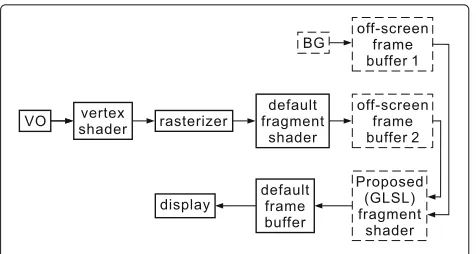
A 3D graphics rendering pipeline employs 3D objects described by their vertices and primitives to generate color values of pixels to be shown on a display. Figure 5

Fig. 5The GPU rendering pipeline

illustrates a general GPU rendering pipeline in solid lines and the proposed GLSL (OpenGL Shader Language) frag-ment shader in dashed lines.

In MR applications, we denote VO for the virtual object and BG for the background to which the virtual object is merged. In case of composition applications, the input image is considered as VO, while there is no BG. Without lost of generality, we explain the rendering pipeline only for the MR case.

In general, raw vertices and primitives of a VO inputted to a vertex shader are processed and transformed for a ras-terizer. The rasterizer scans and converts the transformed primitives into 3D fragments, which are then processed in the default fragment shader and merged to obtain tex-tured and lighten 2D fragments. Normally, the resulting 2D fragments are stored in a default frame buffer and then go to the display. We propose to employ one off-screen frame buffer for storing the 2D fragments of the VO coming from the default fragment shader and another off-screen frame buffer for storing the captured real scene that we will call BG. Since the aerial perspective rendering of Eq. (10) is an RGB-based model, we implement it on a GPU at a fragment level. We insert the fragment shader between the two off-screen buffers and the default frame buffer in order to render a MR frame where the VO has a synthesized aerial perspective effect seamlessly to the natural atmospheric effect visualized on BG.

6.2 Proposed GLSL fragment shader

Fig. 6Proposed GLSL fragment shader for rendering with aerial perspective effect

IVOis given by the RGB values of the CG model textured and illuminated without aerial perspective effect.

Using the abovementioned parameters, the GLSL frag-ment shader consists of the following steps:

1) Initialization: The program calls the texturesIVOand IBG, the target’s relative depth¯s∈[0, 1]and position

(lx,ly) in 2D screen coordinates, the turbidityT, and the spectral sensitivityqc.

2) Positioning: The target’s absolute position in world coordinates is estimated by

s=snear/(1− ¯s(1−snear/sfar)), (19)

φ=arctan(y/x), (20)

θ=arccos(z/

x2_+y2_+z2_{), (21)} where the depths is in meters;snearandsfarare the

distances of near and far planes, respectively; and (x,y,z) is the target’s relative position in world coordinates computed from

⎡ ⎢ ⎢ ⎣

x y z w

⎤ ⎥ ⎥

⎦=[M4×4×P4×4×R4×4]−1

⎡ ⎢ ⎢ ⎣

lx

ly ¯

s

1

⎤ ⎥ ⎥

⎦, (22)

whereM and P are the model view matrix and the projection matrix, respectively, and R is the remap matrix given by

R4×4=

_{2 0 0−1}

0 2 0−1 0 0 2−1 0 0 0 1

. (23)

3) Aerial perspective rendering: The attenuation factor c(T,s)is computed using Eq. (11).Ic∞(T,φ,θ)is computed according to Eqs. (12) and (13). The target with aerial perspective effectIˆVOis calculated using

Eq. (10) and then blended withIBGto produce the

final result.

7 Experimental results

In this section, we evaluated the turbidity estimation approach and the aerial perspective rendering model. Composition application was used for qualitative and quantitative evaluation of the method. We also provide an application on mixed reality. All the following exper-iments were run on C++ on a PC with OS: Windows 7; CPU: Corei7 2.93 GHz; RAM: 16 GB; GPU: nVIDIA GTX 550 Ti 4049 MB.

7.1 Turbidity estimation test

We tested our approach for turbidity estimation using static omnidirectional images of both simulated skies and captured skies.

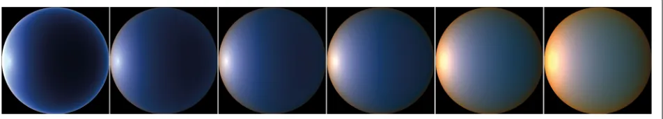
7.1.1 Evaluation with sky models

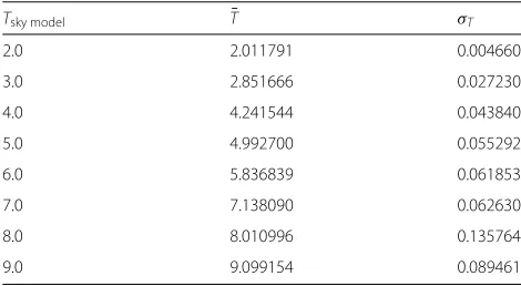
We estimated turbidity 100 times taking Preetham sky models as input images. For this purpose, we implemented the Preetham sky models, which are illustrated in Fig. 7. These models are sky images of 500 by 500 pixels with different values of turbidity ranging from 2.0 to 9.0 and sun position θs = 58.4° and φs = −179.4°. The atmo-spheric turbidity was estimated for each input image using Eq. (8). N = 100 random sampling points were taken for each turbidity estimation. The results are shown in Table 1, where T¯ stands for the mean value of turbidity andσT stands for the corresponding standard deviation.

The speed of the turbidity estimation method was 200 sampling points/second.

7.1.2 Evaluation with captured sky images

We estimated turbidity for omnidirectional sky images captured by Canon EOS5D with a fisheye lens at 12 p.m. in different days. The sky images are illustrated in Fig. 8.

N = 100 random sampling points were used for each turbidity estimation. Turbidity was estimated 50 times for each sky image.

Table 1Estimated turbidity values using the Preetham sky models as an input image

Tsky model T¯ σT

2.0 2.011791 0.004660

3.0 2.851666 0.027230

4.0 4.241544 0.043840

5.0 4.992700 0.055292

6.0 5.836839 0.061853

7.0 7.138090 0.062630

8.0 8.010996 0.135764

9.0 9.099154 0.089461

7.2 Aerial perspective model evaluation

7.2.1 Evaluation of the scattering coefficients

From the proposed corrections, under standard condi-tions (λ=550 nm andh0=0 m), ourβˆMis approximately

70 times smaller than theβMof [3] and roughly 1.43 times

smaller than the corrected Mie scattering coefficient of [13]. We can compare the impact of the Mie scattering coefficient on the aerial perspective effect. To this end, we can employ the approximated values of the attenua-tion factor of [3, 13] and ours, given bye−βscs,e−0.01βscs, and e−0.0137βscs_{, respectively. The results illustrated in}

Fig. 9 show that our attenuation is weaker than Preetham’s attenuation but stronger than Zhao’s attenuation.

We also provide a classification of scattering coefficients through turbidity, as illustrated in Fig. 10. From Eqs. (15) and (18), we have

ˆ

βM1/βˆM2=(T1−1)/(T2−1), (24)

where βˆM1 and βˆM2 refer to our improved Mie scat-tering coefficient for turbidities T1 andT2, respectively. Considering a turbidity of 1.6 for an exceptionally clear atmospheric condition, we plotted Fig. 10 using Eq. (24).

7.2.2 Airlight evaluation

We performed a qualitative evaluation of the airlight constituent of real images using our rendering model of

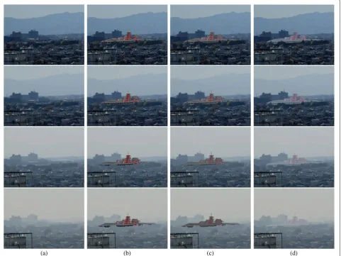
Eq. (10). Real scenes of Tokyo city were captured using Canon EOS5D. The experiments aim to show perfor-mance using a single image as input. Because of this, we used Google earth to manually estimate a rough depth map of the scenes. Nonetheless, depth maps can be esti-mated either from two images of the same scene at different weather conditions using the proposed aerial perspective model or from single images using approaches as in [14, 15]. For a fair evaluation and comparison with state-of-the-art approaches [13–15], the input images were manually segmented to only apply aerial perspective effect over the scene excluding the sky. In addition, the parameters used in the mentioned approaches were set to be optimal.

Figure 11 illustrates our results as well as the results obtained using methods of [13–15] for different atmo-spheric conditions. Theoretically, the airlight component should only contain information from the environmental light affected by the attenuation factor. While our airlight visibly proved to follow such theoretic consistency, the airlights from the other methods clearly retained color information from the target objects.

Moreover, due to the attenuation factor, the more dis-tant the target object is, the more similar to the environ-mental illumination color the airlight should be. Certainly, observing the far way mountains in Fig. 11 we notice that our airlight also followed that theoretic definition, while [13–15] did not succeed to do so.

7.2.3 Evaluation of the aerial perspective effect

In this experiment, we rendered an aerial perspective effect using a given source imageIsand compared the syn-thesized outputIˆtwith a ground truth target imageItof the same scene. We use the subscripts s and t to refer to the source and target, respectively. We dropped the sub-script channel c∈{r,g,b} just for readability; however, the computation was carried out in the three channels. In gen-eral, based on Eq. (10), if we assume constant reflectance properties for objects in the scene, we can first estimate the normalized radiance ρ(x) at pixel x in the source image. Since ρ(x) does not depend on the atmospheric condition, that is

Fig. 9Approximate relation between the attenuation factor of Preetham [3], Zhao [13], and our proposal

ρ(x)= I 0 s(x)

I_s∞(x) =

I_t0(x)

I_t∞(x), (25)

the desired aerial perspective can be applied on the normalized radiance. We compute this two-step process directly by

ˆ

It(x) = Is(x)

I_t∞(x) t(Tt,x)

I_s∞(x) s(Ts,x)

+I_t∞(x)

1− t(Tt,x) s(Ts,x)

, (26)

In the evaluation, we used the input image withTs = 1.9 of Fig. 11 as the source image since it provides more detailed color information than scenes with higher tur-bidities. We targeted to ground truth images withTt = {2.11, 2.54, 2.94, 4.36}.

Figure 12 displays our qualitative results as well as a comparison with results from [13–15]. As can be appre-ciated from the results, our method generated more visually coherent appearances than the state-of-the-art techniques. Synthesized results of all methods were sim-ilar to the ground truth for close objects, such as the biggest building in the scenes. However, while our method prevailed effectively along the entire scene, [13–15] suf-fered from appearance inconsistencies in more distant regions.

Fig. 10Scattering coefficients through turbidity

We also performed a quantitative evaluation using two metrics: the hue saturation brightness (HSV) histogram correlation and the structural similarity (SSIM) image quality index [30] (see Fig. 13). The histogram correlation was calculated as

Corrc(H1,H2)=

c

H1(c)− ¯H1 H2(c)− ¯H2

H1(c)− ¯H1

2

H2(c)− ¯H2

2,

(27)

whereHis histogram,H¯ stands for the histogram mean, c∈{H-S,V}, and lower indexes 1 and 2 correspond toˆItand

It, respectively. In both the HSV correlation and the SSIM index metrics, a higher value represents a higher similarity between the synthesized aerial perspective and the ground truth.

The quantitative results showed that our approach outperformed the methods mentioned beforehand. It is worth noting that while [14] had a better SSIM index than ours only at the least hazy scene, our method provided the highest combined HSV histogram corre-lation for all scenes. In general, at lower turbidities, [14] rendered compelling results closer to ours than [13, 15]. However, contrary to our method, the qual-ity of [13–15] drastically decreased as the haze became denser.

7.3 Application on MR

track-Fig. 11Airlight evaluation with real scenes. Fromtoptobottom rows: scenes with turbiditiesT=1.9,T=2.94, andT=4.36.aInput images. Airlight results ofbHe et al. [14],cZhao [13],dZhu et al. [15], andeours. Depth map intop-left imagewas used only by [13] and our method

ing systems. The altitude at the observer position was

h0 = 40 m above sea level. The distance from the CG model to the observer was around 3500 m. The real scenes of the experiments correspond to the scenes captured for the turbidity estimation test seen in Fig. 8. We use the real scenes with estimated atmospheric turbidities of 1.9, 2.10, 2.94, and 4.36.

The rendered results are shown in Fig. 14. We pro-vide the MR results using Zhao’s method [13] for the comparison. We found that the proposed method synthe-sized more plausible results in terms of visual coherence between the virtual object and the real scene. In terms of computational cost, our rendering speed (14 fps for a full HD frame size) was 225 times faster than Zhao’s method.

Fig. 13Quantitative evaluation of different methods of aerial perspective rendering on real scenes withT=2.11,T=2.54,T=2.94, andT=4.36

8 Conclusions

We have proposed an efficient turbidity-based method for aerial perspective rendering in real scenes. The atmo-spheric turbidity is effectively estimated by matching the luminance distributions of a sky model and an omnidirectional captured sky image. An improved scat-tering model was deduced using real data to classify scattering coefficient values via turbidity. The enhanced

scattering model was employed to provide a novel full-spectrum aerial perspective rendering model. Qualitative and quantitative evaluations on real and synthesized data show that the rendering method accomplishes realistic appearances seamlessly to the natural aerial perspective in real time, outperforming related works in terms of appearance quality and computational cost.

Appendix

Table 2 corresponds to the classification of weather con-ditions based on scattering coefficients. The data was adapted from [16], where measurements were carried out under standard conditions. Standard conditions refer to a spectrally weighted average wavelength (λ=550 nm) for daylight within the visual spectrum at sea level (h=0 m).

Table 2Weather conditions via scattering coefficients

Weather condition βR(km−1) MinβM(km−1) MaxβM(km−1)

Pure air 0.0141 0 0

Exceptionally clear 0.0141 0 0.0639

Very clear 0.0141 0.0639 0.1819

Clear 0.0141 0.1819 0.3769

Light haze 0.0141 0.3769 0.9399

Haze 0.0141 0.9399 1.9459

Fog 0.0141 1.9459 More than 78

Acknowledgements

This work was, in part, supported by JSPS KAKENHI Grant Number 16H05864.

Authors’ contributions

CM, TO, and KI designed the study, developed the methodology, and performed the analysis. CM collected the data. CM wrote the manuscript, and TO and KI helped to polish it. All authors read and approved the final manuscript.

Competing interests

The authors declare that they have no competing interests.

Author details

1_{The University of Tokyo, Tokyo, Japan.}2_{Microsoft Research Asia, Beijing, China.}

Received: 28 July 2016 Accepted: 13 December 2016

References

1. Nishita T, Sirai T, Tadamura K, Nakamae E (1993) Display of the earth taking into account atmospheric scattering. In: Proceedings of the 20th Annual Conference on Computer Graphics and Interactive Techniques, SIGGRAPH’93. ACM, New York. pp 175–182

2. Nishita T, Dobashi Y, Kaneda K, Yamashita H (1996) Display method of the sky color taking into account multiple scattering. In: Proceedings of the Fourth Pacific Conference on Computer Graphics and Applications (Pacific Graphics ’96). pp 66–79

3. Preetham AJ, Shirley P, Smits B (1999) A practical analytic model for daylight. In: Proceedings of the 26th Annual Conference on Computer Graphics and Interactive Techniques, ser. SIGGRAPH ’99. ACM Press/Addison-Wesley Publishing Co., New York. pp 91–100 4. Haber J, Magnor M, Seidel HP (2005) Physically-based simulation of

twilight phenomena. ACM Trans Graphics (TOG) 24(4):1353–73 5. Bruneton E, Neyret F (2008) Precomputed atmospheric scattering.

Comput Graphics Forum 27(4):1079–1086

6. Hosek L, Wilkie A (2012) An analytic model for full spectral sky-dome radiance. ACM Trans Graphics (TOG) 31(4):95

7. Hosek L, Wilkie A (2013) Adding a solar-radiance function to the Hosek-Wilkie skylight model. IEEE Comput Graphics Appl 33(3):44–52 8. Kerker M (1969) The scattering of light and other electromagnetic

radiation. Academic press, New York

9. Kider Jr, Knowlton D, Newlin J, Li YK, Greenberg DP (2014) A framework for the experimental comparison of solar and skydome illumination. ACM Trans Graphics (TOG) 33(6):180

10. Jung J, Lee JY, Kweon IS (2015) One-day outdoor photometric stereo via skylight estimation. In: Proceedings of the IEEE Conference on Computer Vision and Pattern Recognition, Boston. pp 4521–4529

11. Satilmis P, Bashford-Rogers T, Debattista K, Chalmers A (2016) A machine learning driven sky model. In: IEEE Computer Graphics and Applications 12. Wang X, Gao J, Fan Z, Roberts NW (2016) An analytical model for the

celestial distribution of polarized light, accounting for polarization singularities, wavelength and atmospheric turbidity. J Optics 18(6):065601

13. Zhao H (2012) Estimation of atmospheric turbidity from a sky image and its applications. Ph.D. dissertation, Graduate School of Information Science and Technology, The University of Tokyo

14. He K, Sun J, Tang X (2011) Single image haze removal using dark channel prior. IEEE Trans Pattern Anal Mach Intell 33(12):2341–2353 15. Zhu Q, Mai J, Shao L (2015) A fast single image haze removal algorithm

using color attenuation prior. IEEE Trans Image Process 24(11):3522–3533 16. McCartney EJ (1976) Optics of the atmosphere: scattering by molecules

and particles, vol. 1. John Wiley and Sons, Inc., New York, p. 421 17. Dobashi Y, Yamamoto T, Nishita T (2002) Interactive rendering of

atmospheric scattering effects using graphics hardware. In: Proceedings of the ACM SIGGRAPH/EUROGRAPHICS Conference on Graphics Hardware, ser. HWWS ’02. Eurographics Association, Aire-la-Ville, Switzerland. pp 99–107

18. Nielsen RS (2003) Real time rendering of atmospheric scattering effects for flight simulators. Master’s thesis, Informatics and Mathematical Modelling, Technical University of Denmark, DTU, Richard Petersens Plads, Building 321, DK-2800 Kgs. Lyngby

19. Riley K, Ebert DS, Kraus M, Tessendorf J, Hansen C (2004) Efficient rendering of atmospheric phenomena. In: Proceedings of the Fifteenth Eurographics Conference on Rendering Techniques, ser. EGSR’04. Eurographics Association, Aire-la-Ville, Switzerland. pp 375–386 20. Schafhitzel T, Falk M, Ertl T (2007) Real-time rendering of planets with

atmospheres. In: Journal of WSCG 15(1–3). pp 91–98

21. Gao R, Fan X, Zhang J, Luo Z (2012) Haze filtering with aerial perspective. In: 19th IEEE International Conference on Image Processing (ICIP). pp 989–992

22. Narasimhan SG, Nayar SK (2003) Contrast restoration of weather degraded images. Pattern Anal Mach Intell IEEE Trans 25(6):713–724 23. Nayar S, Narasimhan S (1999) Vision in bad weather. In: International

Conference on Computer Vision. pp 820–827

24. Tan R (2008) Visibility in bad weather from a single image. In: Proceedings of IEEE International Conference on Computer Vision and Pattern Recognition. pp 1–8

25. Strutt JW (1871) Lviii. On the scattering of light by small particles. London, Edinburgh Dublin Philos Mag J Sci 41(275):447–454 26. Mie G (1908) Beitrage zur optik truber medien, speziell kolloidaler

metallosungen. Annalen der Physik 330(3):377–445

27. Perez R, Seals R, Michalsky J (1993) All-weather model for sky luminance distribution-preliminary configuration and validation. Solar Energy 50(3):235–245

28. Kawakami R, Zhao H, Tan RT, Ikeuchi K (2013) Camera spectral sensitivity and white balance estimation from sky images. Int J Comput Vis 105(3):187–204

29. Zhao H (2013) Spectral sensitivity database. http://www.cvl.iis.u-tokyo. ac.jp/rei/research/cs/zhao/database.html. Accessed 31 May 2013 30. Wang Z, Bovik A, Sheikh H, Simoncelli E (2004) Image quality