R E G U L A R A R T I C L E
Open Access
Testing the hypothesis of preferential
attachment in social network formation
Thomas House
1,2*, Jonathan M Read
3, Leon Danon
4and Matthew J Keeling
2*Correspondence:
1School of Mathematics, University
of Manchester, Oxford Road, Manchester, M13 9PL, UK
2Warwick Infectious Disease
Epidemiology Research (WIDER), University of Warwick, Gibbet Hill Road, Coventry, CV4 7AL, UK Full list of author information is available at the end of the article
Abstract
The hypothesis of preferential attachment (PA) - whereby better connected individuals make more connections - is hotly debated, particularly in the context of epidemiological networks. The simplest models of PA, for example, are incompatible with the eradication of any disease through population-level control measures such as random vaccination. Typically, evidence has been sought for the presence or absence of preferential attachment via asymptotic power-law behaviour. Here, we present a general statistical method to test directly for evidence of PA in count data and apply this to data for contacts relevant to the spread of respiratory diseases. We find that while standard methods for model selection prefer a form of PA, careful analysis of the best fitting PA models allows for a level of contact heterogeneity that in fact allows control of respiratory diseases. Our approach is based on a flexible but numerically cheap likelihood-based model that could in principle be applied to other integer data where the hypothesis of PA is of interest.
Keywords: MLE; Phase-type distribution; model selection; spectral methods
1 Introduction
1.1 Contact heterogeneity in infectious disease epidemiology
Infectious pathogens that spread via contact between people are a major cause of human disease, driving attempts to understand their epidemiology []. Much theoretical work on infectious disease dynamics has been focused on the role of heterogeneity in the human population [], which is often conceptualised as a network of epidemiologically relevant contacts [–].
Perhaps the most important quantity in any infectious disease outbreak is the basic re-productive ratio,R, which is defined verbally as the expected number of secondary cases
generated by an average primary case early in the epidemic. An epidemic is possible exactly whenR> , and typically the efforts required to control such an outbreak grow
mono-tonically withR[, ]. In the simplified scenario where each individual picks an integer
number of contactsKfrom the samedegree distribution, but transmission is otherwise
homogeneous,
R∝E
K. ()
This dependence of the basic reproductive ratio on the second moment of the degree dis-tribution has been a ‘textbook’ result for some time [], however work by Pastor-Satorras and Vespignani [] and May and Lloyd [] raised the question of what might happen for large, or asymptotically divergent, second moments. Such questions can be posed and answered at different levels of mathematical rigour [] however in the context of epidemi-ology it is clear that a highly variable degree distribution is associated with the epidemio-logically unrealistic scenario that even the most weakly transmissible pathogen can cause an epidemic, and as a corollary that control of any infectious disease through untargeted vaccination would be impossible.
1.2 Data
Of course, whether such a theoretical possibility matters for the study of infectious dis-eases depends on the actual variance in degree for epidemiologically relevant contacts. While th century models of infectious disease were often based on strong a priori as-sumptions about mixing patterns [], various methods for measurement of contact pat-terns now exist and were reviewed by Read et al. []. As well as direct measurement of individuals through surveys [] it is possible to improve coverage through snowball and respondent-driven sampling [, ], to make use of the extremely large datasets produced by electronic sensors [, ], and also to combine aggregate data [, ].
Previous empirical studies have seen evidence that for direct (e.g. [, ]) and sexual (e.g. [, ]) contacts, an approximate power-law relationship may hold such that for largek, a randomly selected node obeys
Pr(node hasklinks)≈k–γ. ()
As is the case for almost all biological data, there is much more complexity in the data than such a simple parametric relationships as () would imply. For example, Leigh Brown et al. [] found that while a power-law was a better functional form than the negative binomial for sexual contacts, the richer Waring distribution was preferable to either. What is hard to dispute, however, is that as better quality data on epidemiologically relevant contacts is obtained the evidence consistently points to a very high level of variance; for example, Read et al. [] were able to validate the high numbers of contacts reported by some study participants through direct (rather than postal) surveying.
These empirical observations of high heterogeneity in contact number, together with theoretical results aboutR, present a paradox for infectious disease epidemiology: is the
extreme heterogeneity in observed contact patterns indicative of PA and does that im-ply that R> for almost any finite level of person-to-person transmissibility meaning
that our theoretical understanding of infectious disease epidemiology is somehow severely lacking?
1.3 Preferential attachment and power laws in empirical data
attachment is intimately linked with, but not always equivalent to, asymptotic power-law behaviour.
Simple power-law relationships have been claimed for numerous real-world systems, and a critical review of these claims by Clauset et al. [] used maximum-likelihood fitting of distribution tails to power-law distributions to show varying levels of statistical support for claims in the literature. In the context of discrete data, pioneering work by Zipf []
found power-laws in word frequencies; considering the count of unique words inMoby
Dickboth Newman [] and Clauset et al. [] agree that the statistical evidence for Zipf ’s power-law distribution in this context is strong. On the other hand, the in- and out-degrees ofE. colimetabolic networks have been claimed to follow a power law [], but this is disputed by the analyses of Huss and Holme [] and Clauset et al. [].
The debate around presence or absence of power laws in real data continues, perhaps most strongly in the context of networks. For example, Barabási [] writes that prefer-ential attachment is network science’s “most profuse concept,” and that “the impact of preferential attachment is hard to miss.” At the same time, Stumpf and Porter [] argue that “most reported power laws lack statistical support and mechanistic backing.”
1.4 Testing preferential attachment directly
In this work, we attempt to test the hypothesis of preferential attachment in social con-tact data directly, rather than via asymptotic power law behaviour. We make use of previ-ously collected data on social encounters specifically designed to measure heterogeneity in numbers of contacts amongst the British population, and fit mechanistic models of different complexity to these data. We determine that models with significant levels of preferential attachment have better evidential support from the data than models with-out.
2 Methods
2.1 Social Contact Survey data
A cross-sectional study was conducted between May and October , recruiting households and individuals through postal and online questionnaires, supported by a large random-address mailshot and a modest online and media promotion [, ]. Question-naires asked respondents to report on the number of distinct individuals they encountered the previous day: their contacts. Respondents were able to report contacts either as indi-viduals or as members of a group with a reported size. Allowing the reporting of groups of individuals was a deliberate methodological design to permit the easy reporting of large numbers of contacts, to avoid the approach taken by previous studies [], which imposed a high burden on respondents with large number of contacts, and to ensure the best cap-ture of the right-hand tail of the degree distribution. In general, we expect that such data will become increasingly available due to the epidemiological importance of this tail (e.g. the study of Read et al. []).
2.2 Generalised preferential attachment
As noted by Durrett [], Barabási [], and Simkin and Roychowdhury [], the basic idea behind the preferential attachment model is close to the population model of Yule []. We consider a Yule-like stochastic process described precisely as follows. In a population ofNindividuals indexed byieach individual has an integer-valued random variableKi(t) for its number of contacts. Individualistarts withKi() = and makes new contacts over a time periodTi, which is given by a positive real-valued random variable with probability density functionρ(t). The generation of new social contacts is modelled by a continuous-time Markov chain with the following events and rates:
Ki→Ki+ at ratefKi:= +τKi. ()
We take the preferential attachment hypothesis PA to be stated mathematically as
PA⇔τ > . ()
Writingpk(t) for the probability thatKi=kat timet<Ti, we can use the method of char-acteristics to derive an expression for the probability generating function ofKi,
g(t,s) = k
pk(t)sk=
s– (s– )eτt–/τ
, s∈[, ]. ()
From this, we can derive expressions for the probability mass function,
pk(t) =
k!
∂kg
∂sk
s=
= (k+
τ) τ (
τ)(k+ )
e–teτt– k
→κt
eτt– kk(–τ)/τ, ()
whereκtis a function oftbut notkand the asymptote holds askbecomes large. This is not a simple power-law relationship, and so the asymptotic behaviour of the moments is not determined by the power-law exponent, but rather through the moment generating functionM(t,z) =g(t, ez),z∈(–∞, ], such that therth moment of the degree distribution, conditional ont<T, is
mr(t) =
∂rM
∂zr
z=
. ()
In particular,
m(t) =
τ
eτt– , m(t) =m(t) + (τ+ )
m(t)
, . . . . ()
Then accounting for the randomness of the times, therth moment of the degree distribu-tion will be
mr=
∞
t=
ρ(t)mr(t) dt. ()
Figure 1 A model ofmphases.νais the probability of starting in
phasea,μais the exit rate of phasea, andQa,bis the rate of moving
from phaseato phaseb.
2.3 Phase-type holding times
The question is then posed as to an appropriate distribution from which to draw the
hold-ing times{Ti}for the amount of time spent making new contacts on the day for which
individuals provide data. In previous work [] on a related model of contact formation we considered holding timesTithat were log-normally distributed. This provided a good fit to data, but was computationally intensive and lacked a mechanistic interpretation. We therefore consider here a class of distributions for the holding times that is highly flexi-ble, but which has analytic and numerical benefits - the distributions ofphase type[]. Phase-type distributions are dense in the space of positive-valued probability distributions [], meaning that they can be made arbitrarily close to any other distribution. They have a mechanistic interpretation and allow for analytic manipulations that greatly reduce the numerical cost of likelihood evaluation.
The basic idea behind the model is shown in Figure . A set of phases is indexed bya,b= , . . . ,m; the probability of starting in phaseaisνa(meaning these parameters must sum to unity); the rate of stopping making new social contacts isμafor an individual in phasea; and the rate of moving from phaseato phasebisQa,b. Note that different rates of making contacts in different phases are not realistically distinguishable from different times spent and so are not included as parameters. The phases have a mechanistic interpretation as the activities that individuals undertake on a given day.
In this model, the probability density function for the holding time is given by the general expression
ρ(t) =μeMtν, ()
where:
μ= (μa); ν= (νa);
Ma,a= –Ma; Ma=μa+
b
Qb,a; Ma,b=a=Qb,a.
()
From the expressions (), (), () and () above, in particular through inspection of the
form of the moment generating function, it is clear that the rth moment of the degree
distribution will involve a term like
Ir=
∞
t=
erτtρ(t) dt=μ ∞
t=
e(M+rτI)tdtν, ()
λa= –Ma+rτ. If we let R be a matrix whoseath column is theath right eigenvector of A and L be a matrix whoseath row is theath left eigenvector of A then
Ir=μ ∞
t=
L–LeAtRR–dtν=μL– ∞
t=
DdtR–ν, ()
where D is a diagonal matrix whoseath diagonal element is eλat. The integralIrtherefore converges exactly when∀a,λa< , which implies that the condition for divergence of the
rth moment is
mrdiverges ⇔ ∃asuch thatτ>Ma/r. ()
In general, however, combination of () and () is not the most numerically efficient method for calculation of the overall probability mass function for final number of con-tactsKi(Ti) and a different approach is needed.
2.4 Numerically efficient model solution
The model as described above can be solved in a numerically efficient manner using the spectral methods for continuous-time Markov chains developed by Bailey []. We
con-sider the limit as the population sizeN→ ∞and write down ordinary differential
equa-tions (ODEs) for the proportion of the population in phaseaand withksocial contacts at timet,pa,k(t). These ODEs take the form
d
dtpa,k= – fk+μa+
b>a
Qa,b
pa,k+fk–pa,k–+
b<a
Qb,apb,k, ()
wherefkis the rate at which individuals withksocial contacts make new contacts, given in (). We are then interested indk, the probability mass function for a randomly selected in-dividual having madeksocial contacts by the end of the process. A series of manipulations directly analogous to those of Bailey [] shows that
dk=lim s↓
a
μa
∞
e–stpa,k(t) dt=:
a
μaAa,k. ()
Applying Laplace transformation to () subject to the initial conditionpa,k() =νaδk,
and taking the frequency-space limits↓ then leads to a set of linear equations fordk that are triangular and so can be evaluated directly without numerically costly matrix in-version:
νaδk,= – fk+μa+
b>a
Qa,b
Aa,k+fk–Aa,k–+
b<a
Qb,aAb,k. ()
2.5 Model likelihood, fitting and selection
We assume a vector of data y = (yk), whereyk is the number of individuals reportingk
social contacts when surveyed. A modelMis therefore specified by a number of phasesm
and the presence or absence of PA, meaning the general parameters areθ= (τ,νa,μa,Qa,b), withτ present only if there is PA. The numbernof individuals sampled from the British populationNis
n= k
yk= N×, ()
and so it is appropriate to assume that each individual picks a number of contacts indepen-dently from the distribution with pmf given bydkas in (). Accounting for the censoring of zero contacts in the real data, we define
˜
d= , d˜k>=
dk –d
, ()
meaning that the overall likelihood function is then given by
L(y|θ) =n! lyl!
k
˜
dk(θ)yk
. ()
Note that the combinatorial factors do not depend on the parameters, and so need not be calculated during model fitting.
We consider the use of the likelihood function () using standard statistical methodol-ogy. Numerical maximum likelihood estimation was performed using simulated anneal-ing run from multiple startanneal-ing points to ensure the global optimum was obtained. Model selection was performed using AIC [] and BIC [], as well as likelihood ratio tests [] on pairs of models where this test was informative. This was done since each ap-proach involves different trade-offs between model fit and complexity, and to check that our conclusions about PA are not overly sensitive to the precise method used. Uncer-tainty in model parameters was quantified using confidence intervals obtained through bootstrapping the data, and uncertainty in model outputs such as the predicted degree distribution was quantified using a parametric bootstrap.
3 Results and discussion
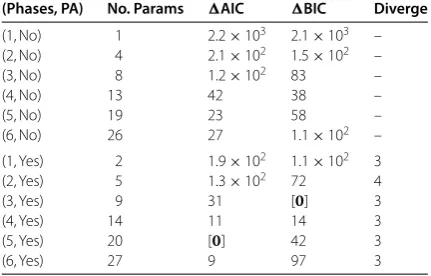
Table shows the models we fitted, their number of parameters, AIC/BIC relative to the minimum, and the first moment that diverges according to (). Figure shows the results of performing likelihood ratio tests. These show that AIC prefers a -phase model with PA as do likelihood ratio tests for any significance level between .% and %. BIC penalises complex models more severely and therefore selects a -phase model with PA.
Table 1 Comparison of models with different numbers of phases, with and without
preferential attachment (PA), together with: number of parameters; differences in AIC and BIC values compared to the overall minimum; and the lowest divergent moment for models with PA
(Phases, PA) No. Params AIC BIC Diverge
(1, No) 1 2.2×10³ 2.1×10³ –
(2, No) 4 2.1×10² 1.5×10² –
(3, No) 8 1.2×10² 83 –
(4, No) 13 42 38 –
(5, No) 19 23 58 –
(6, No) 26 27 1.1×10² –
(1, Yes) 2 1.9×10² 1.1×10² 3
(2, Yes) 5 1.3×10² 72 4
(3, Yes) 9 31 [] 3
(4, Yes) 14 11 14 3
(5, Yes) 20 [] 42 3
(6, Yes) 27 9 97 3
Preferred models are shown using square brackets and bold type.
Figure 2 The results of likelihood ratio tests on the models.
Arrows point towards the model preferred by the likelihood ratio test, withpvalues shown.
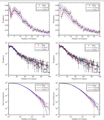
For the -phase model with PA,τ= . [., .]; and if we setτ= but leave the other parameters at their fitted values, then the total number of contacts per person is re-duced to % of its original value. For the -phase model with PAτ= . [., .]; and if we setτ= but leave the other parameters at their fitted values, then the total num-ber of contacts per person is reduced to % of its original value. This shows that in both of these models, we can attribute a substantial fraction of the contacts to PA.
We also calculate that the second moment does not diverge in any of the fitted mod-els, which helps to resolve the epidemiological paradox that we introduced at the start of this paper. PA is empirically supported, and is also mechanistically plausible since existing social contacts give more opportunities for future social contact. Combined with a suffi-ciently detailed phase-based mechanistic model of the contexts in which social contacts are made, however, PA does not imply a divergent second moment for the distribution of contacts relevant for the spread of directly transmitted infections. This means that our un-derstanding of how basic epidemiological quantities like the basic reproductive ratio,R,
Figure 3 Data at different scales versus (left column) model selected using AIC and likelihood ratio tests (right column) model selected using BIC.Models are labelled by the number of phases and whether PA is present. Confidence intervals in the data are calculated using bootstrapping for data and parametric bootstrapping for models.
As a final observation, we believe that as computational resources for fitting models to data improve, it will in general be easier to test the hypothesis of PA directly in all kinds of data, rather than looking for asymptotic power laws.
Appendix A: Code
We provide the function phase_ll.c below as a Mex file for use within MATLAB; how-ever, the C syntax is standard and modification to run within R, Python or C should be straightforward. Once compiled, use within MATLAB is:
>> [LL, P] = phase_ll(params,M,kh,K);
whereparamsis a vector of the model parameters[nu(:), mu(:), Q(:), tau],
count,LLis the log-likelihood given the parameters andPis a the probability vector for the observed counts given the parameters.
A.1 The function phase_ll.c
#include <mex.h> #include <math.h>
void mexFunction (int nlhs, mxArray *plhs[], int nrhs, const mxArray *prhs[]) {
/* Input variables */
double *params, *kh, *Mmex, *Kmex; size_t lp;
int M, K;
/* Get inputs in correct form */ params = mxGetPr(prhs[0]); lp = mxGetN(prhs[0]); Mmex = mxGetPr(prhs[1]); kh = mxGetPr(prhs[2]); Kmex = mxGetPr(prhs[3]); M = (int) Mmex[0]; K = (int) Kmex[0];
/* Working variables */
double nu[M], mu[M], Q[M][M], s[M]; double f[K];
double tau, S; double A[K][M]; int fi, fj, k, m;
/* Output variables */ double *P, *LL;
/* Organise outputs into correct form */ plhs[0] = mxCreateDoubleMatrix(1,1,mxREAL); LL = mxGetPr(plhs[0]);
plhs[1] = mxCreateDoubleMatrix(K,1,mxREAL); P = mxGetPr(plhs[1]);
nu[0] = 1.0;
for(fi=1; fi<M; fi++) { nu[fi] = params[fi-1]; nu[0] -= params[fi-1]; }
for(fi=M; fi<(2*M); fi++) { mu[fi-M] = params[fi-1]; }
m = (2*M)-1;
for(fi=0; fi<M; fi++) { s[fi] = 0;
Q[fi][fj] = params[m]; s[fi] += params[m]; m=m+1;
} }
if (lp == (m+1)) tau = params[m]; else
tau = 0;
f[0] = 1;
for(k=1; k<(K-1); k++) f[k] = 1+(tau*k); f[K-1] = 0;
A[0][0] = (nu[0])/(f[0]+mu[0]+s[0]); for(k=1; k<K; k++) {
A[k][0] = ( f[k-1]/(f[k]+mu[0]+s[0]) )*A[k-1][0]; }
for(m=1; m<M; m++) { S=0.0;
for(fi=0; fi<m; fi++) { S += Q[fi][m]*A[0][fi]; }
A[0][m] = (nu[m]+S)/(f[0]+mu[m]+s[m]); for(k=1; k<K; k++) {
S=0.0;
for(fi=0; fi<m; fi++) { S += Q[fi][m]*A[k][fi]; }
A[k][m] = ((f[k-1]*A[k-1][m])+S)/(f[k]+mu[m]+s[m]); }
}
P[0] = 0.0;
for(m=0; m<M; m++) { P[0] += A[0][m]*mu[m]; }
for(k=1; k<K; k++) { P[k] = 0.0;
for(m=0; m<M; m++) { P[k] += A[k][m]*mu[m]; }
P[k] /= (1-P[0]); }
P[0] = 0.0;
LL[0] = 0.0;
for(k=1; k<(K-1); k++) { LL[0] += kh[k]*log(P[k]); }
Competing interests
The authors declare that they have no competing interests.
Authors’ contributions
All authors: collected the data, designed the study. TH: performed the analysis.
Author details
1School of Mathematics, University of Manchester, Oxford Road, Manchester, M13 9PL, UK.2Warwick Infectious Disease
Epidemiology Research (WIDER), University of Warwick, Gibbet Hill Road, Coventry, CV4 7AL, UK. 3CHICAS, Faculty of
Health and Medicine, Lancaster University, Lancaster, Lancashire, LA1 4YG, UK.4School of Social and Community
Medicine, University of Bristol, Oakfield Grove, Clifton, BS8 2BN, UK.
Acknowledgements
The Social Contact Survey was funded by the Medical Research Council, grant number G0701256. TH and MJK are supported by the Engineering and Physical Sciences Research Council. JMR and MJK are supported by the Economic and Social Research Council, grant ES/K004255/1. LD is supported by the Leverhulme Trust.
Received: 2 July 2015 Accepted: 28 September 2015 References
1. Anderson RM, May RM (1991) Infectious diseases of humans. Oxford University Press, Oxford
2. Diekmann O, Heesterbeek JAP, Britton T (2012) Mathematical tools for understanding infectious disease dynamics. Princeton University Press, Princeton
3. Bansal S, Grenfell BT, Meyers LA (2007) When individual behaviour matters: homogeneous and network models in epidemiology. J R Soc Interface 4(16):879-891
4. Danon L, Ford AP, House T, Jewell CP, Keeling MJ, Roberts GO, Ross JV, Vernon MC (2011) Networks and the epidemiology of infectious disease. Interdiscip Perspect Infect Dis 2011:284909
5. Pellis L, Ball F, Bansal S, Eames K, House T, Isham V, Trapman P (2014) Eight challenges for network epidemic models. Epidemics 10:58-62. doi:10.1016/j.epidem.2014.07.003
6. Diekmann O, Heesterbeek JAP (2000) Mathematical epidemiology of infectious diseases: model building, analysis and interpretation. Wiley, New York
7. Pastor-Satorras R, Vespignani A (2001) Epidemic dynamics and endemic states in complex networks. Phys Rev E 63:066117
8. May RM, Lloyd AL (2001) Infection dynamics on scale-free networks. Phys Rev E 64:066112
9. Durrett R (2010) Some features of the spread of epidemics and information on a random graph. Proc Natl Acad Sci USA 107(10):4491-4498
10. Read JM, Edmunds WJ, Riley S, Lessler J, Cummings DAT (2012) Close encounters of the infectious kind: methods to measure social mixing behaviour. Epidemiol Infect 140(12):2117-2130
11. Mossong J, Hens N, Jit M, Beutels P, Auranen K, Mikolajczyk R, Massari M, Salmaso S, Tomba GS, Wallinga J, Heijne J, Sadkowska-Todys M, Rosinska M, Edmunds WJ (2008) Social contacts and mixing patterns relevant to the spread of infectious diseases. PLoS Med 5(3):381-391
12. Goodman LA (1961) Snowball sampling. Ann Math Stat 32:148-170
13. Heckathorn DD (1997) Respondent-driven sampling: a new approach to the study of hidden populations. Soc Probl 44:174-199
14. Salathé M, Kazandjieva M, Lee JW, Levis P, Feldman MW, Jones JH (2010) A high-resolution human contact network for infectious disease transmission. Proc Natl Acad Sci USA 107(51):22020-22025
15. Isella L, Stehlé J, Barrat A, Cattuto C, Pinton J, Van den Broeck W (2011) What’s in a crowd? Analysis of face-to-face behavioral networks. J Theor Biol 271(1):166-180
16. Eubank S, Guclu H, Kumar VSA, Marathe MV, Srinivasan A, Toroczkai Z, Wang N (2004) Modelling disease outbreaks in realistic urban social networks. Nature 429(6988):180-184
17. Eubank S, Barrett C, Beckman R, Bisset K, Durbeck L, Kuhlman C, Lewis B, Marathe A, Marathe M, Stretz P (2010) Detail in network models of epidemiology: are we there yet? Journal of Biological Dynamics 4(5):446-455
18. Fournet J, Barrat A (2014) Contact patterns among high school students. PLoS ONE 9(9):e107878
19. Schneeberger A, Mercer CH, Gregson SAJ, Ferguson NM, Nyamukapa CA, Anderson RM, Johnson AM, Garnett GP (2004) Scale-free networks and sexually transmitted diseases: a description of observed patterns of sexual contacts in Britain and Zimbabwe. Sex Transm Dis 31(6):380-387
20. Leigh Brown AJ, Lycett SJ, Weinert L, Hughes GJ, Fearnhill E, Dunn DT (2011) Transmission network parameters estimated from HIV sequences for a nationwide epidemic. J Infect Dis 204(9):1463-1469
21. Read JM, Lessler J, Riley S, Wang S, Tan LJ, Kwok KO, Guan Y, Jiang CQ, Cummings DAT (2014) Social mixing patterns in rural and urban areas of southern China. Proc R Soc B 281(1785):20140268
22. Barabási AL, Albert R (1999) Emergence of scaling in random networks. Science 286(5439):509-512 23. Clauset A, Shalizi CR, Newman MEJ (2009) Power-law distributions in empirical data. SIAM Rev 51(4):661-703 24. Zipf GK (1949) Human behavior and the principle of least effort: an introduction to human ecology. Addison-Wesley,
Reading
25. Newman MEJ (2005) Power laws, Pareto distributions and Zipf’s law. Contemp Phys 46(5):323-351
26. Jeong H, Tombor B, Albert R, Oltvai ZN, Barabási AL (2000) The large-scale organization of metabolic networks. Nature 407(6804):651-654
27. Huss M, Holme P (2007) Currency and commodity metabolites: their identification and relation to the modularity of metabolic networks. IET Syst Biol 1(5):280-285
28. Barabási AL (2012) Network science: luck or reason. Nature 489(7417):507-508
29. Stumpf MPH, Porter MA (2012) Critical truths about power laws. Science 335(6069):665-666
31. Danon L, Read JM, House T, Vernon MC, Keeling MJ (2013) Social encounter networks: characterizing Great Britain. Proc R Soc B 280(1765):20131037
32. Durrett R (2007) Random graph dynamics. Cambridge University Press, Cambridge 33. Simkin MV, Roychowdhury VP (2011) Re-inventing Willis. Phys Rep 502(1):1-35
34. Yule GU (1925) A mathematical theory of evolution, based on the conclusions of Dr. J. C. Willis, F.R.S. Philos Trans R Soc Lond B, Contain Pap Biol Character 213:21-87
35. Neuts MF (1981) Matrix-geometric solutions in stochastic models: an algorithmic approach. Johns Hopkins University Press, Baltimore
36. Neuts MF (1975) Probability distributions of phase type. In: Liber amicorum Professor emeritus Dr. H. Florin. Katholieke Universiteit Leuven, Departement Wiskunde, Leuven, pp 173-206
37. Bailey NTJ (1957) The mathematical theory of epidemics. Griffin, London
38. Akaike H (1974) A new look at the statistical model identification. IEEE Trans Autom Control 19(6):716-723 39. Schwarz G (1978) Estimating the dimension of a model. Ann Stat 6(2):461-464