R E S E A R C H
Open Access
Performance evaluation of data aggregation for
cluster-based wireless sensor network
Adwitiya Sinha
*and Daya Krishan Lobiyal
* Correspondence: [email protected] School of Computer & Systems Sciences, Jawaharlal Nehru University, New Delhi, India
Abstract
In wireless sensor network, data fusion is considered an essential process for preserving sensor energy. Periodic data sampling leads to enormous collection of raw facts, the transmission of which would rapidly deplete the sensor power. In this paper, we have performed data aggregation on the basis of entropy of the sensors. The entropy is computed from the proposed local and global probability models. The models provide assistance in extracting high precision data from the sensor nodes. We have also proposed an energy efficient method for clustering the nodes in the network. Initially, sensors sensing the same category of data are placed within a distinct cluster. The remaining unclustered sensors estimate their divergence with respect to the clustered neighbors and ultimately join the least-divergent cluster. The overall performance of our proposed methods is evaluated using NS-2 simulator in terms of convergence rate, aggregation cycles, average packet drops, transmission cost and network lifetime. Finally, the simulation results establish the validity and efficiency of our approach.
Keyword:Wireless sensor network; Divergence clustering; Entropy-based data aggregation; Local and global aggregation
Introduction
The wireless sensor network (WSN) [1] has started receiving huge research incentives for its omnipresence in several applications, including environmental monitoring, wildlife exploration, medical supervision and battlefield surveillance. The sensor network is formed with small electronic devices possessing self-configuring capability that are either randomly deployed or manually positioned in huge bulk [2]. It performs activities in several dimensions, for instance identifying the neighborhood, presence of targets or monitoring environmental factors (motion, temperature, humidity, sound and other physical variables). However, owing to limited battery power, the sensor networks demand energy efficient resolutions to enhance the performance of sensor network.
Energy consumption problem, being the most visible challenge, is considered central to the sensor research theme. The processing of data, memory accesses and input/output operations, all consume sensor energy. However, the major power drain occurs due to wireless communication [3]. Therefore, attempts require to be carried out to perform as much in-network processing as possible within a sensor or a group of sensors (cluster). This is achieved by performing aggregation and filtration of raw data before transmitting them to destined targets. As a result of which redundancy in the recorded sensory
samples is eliminated, thereby reducing the transmission cost and network overloading. Moreover, decrease in the effective number of packet transmissions also leads to minimized chances of network congestion, thereby saving the excess energy consumption in the network. For instance, if the radio electronics requires 50nJ/bit and amplifier circuitry needs 10pJ/bit/m2 for communication, then power used in transmitting 1 bit of information to the processing center situated 1 km away, consumes 1.005 × 10⁴ nJ per unit time (watts). However, energy used in data processing for aggregation is 5 nJ/bit/signal, which implies that execution of almost 2010 instructions compensates the energy used for one transmission in unit time. Therefore, it is quite recommendable to apply aggregation techniques. Previous researches have already proven the fact that in-network processing cost is much less than the communication cost [4-14].
The proliferation of sensor network has created the urge of exploring novel ideas for data aggregation. However, the aggregation schemes would require efficient clustering protocols to well-implement its functioning. Hence, in this paper we have contributed a divergence-measure based clustering protocol along with entropy based data aggregation, to the ongoing sensor network research. The remainder of this paper is organized as follows: a brief review of previous research carried out in the related field is included in section 2. Our proposed clustering technique based on divergence measure is provided in section 3. In section 4, the proposed fuzzy-entropy based aggregation scheme has been elaborated. Analysis of network diagram is presented in section 5. Section 6 shows the performance evaluation of our proposed method. Finally, the paper is concluded in section 7 along with directions for further scope.
Related work
The energy consumption in wireless sensor network has created enormous awareness among the researchers for increasing the network lifetime. The sensor network is considered to have prospective results in terms of dynamism and diversity in everyday applications. Several resource efficient protocols have been introduced by researchers in order to limit the sensor energy usage, at the same time maintaining a sufficient degree of reliability and throughput.
dynamically and updated on sensing environmental parameters followed by aggre-gation at the cluster head. The clusters formed in this case, are also known as adaptive clusters.
An energy aware algorithm has been provided in [4] for constructing an aggregation tree prior to data transmission. The algorithm seems to reflect the influence of both the energy and distance parameters to construct the tree. In another research [5], the authors have performed aggregation by considering entropy of correlated data transmitted by the source nodes. This procedure reduces the amount of redundant data forwarded to the sink. Furthermore, the estimation of joint entropy of the correlated data set helps in maximizing information integrity. Another interesting aggregation protocol is developed in [6] on the basis of wavelet-entropy. Initially, multi-scale wavelet transforms are used to spread signals in multi-scale range, after which information is aggregated using wavelet-entropy discriminance theorem. Simulation results indicate that the proposed method is capable to extend the lifetime of networks to a much greater degree than Low-Energy Adaptive Clustering Hierarchy (LEACH) protocol [7]. In [8] the authors have put forward a novel approach that focusses on data aggregation with significantly reduced aggregation latency. Collision-free schedule is generated by a distributed algorithm for performing data aggregation in wireless sensor network. The time latency of aggregation schedule is minimized using greedy strategy.
In a recent research [9], an aggregation scheme called smart aggregation is developed for continuous monitoration in sensor networks. The proposed technique maintains a tolerable deviation (a bounded error) in the aggregated data while utilizing the spatio-temporal correlation of data. In another subsequent work [10], data aggregation techniques are designed on the basis of statistical information extraction. The applied methods exhibits bounded message overhead and robustness against link failures. The expectation–maximization (EM) algorithm is used in order to accomplish accurate estimation of distribution parameters of sensory data. The experimental outcome confirms reduced network communication cost even in large scale sensor networks. In a latest publication [11], the corresponding authors have presented α-local spatial clustering algorithm along with data aggregation mechanism. The contribution was mainly made for environmental surveillance applications in high density sensor networks. The aggregation algorithm constructs a dominating set by exploiting the spatial correlation between data measured by different sensors. The dominating set is further considered as network backbone to execute data aggregation on the basis of information summarization of the dominator nodes. Another research in [12] proposed cooperative information aggregation (CIA) mechanisms to handle observation noise and communication errors initially found in the sampled data. Moreover, the authors have designed an aggregation hard decision estimator (AHDE) and an Aggregation Maximum-Likelihood Estimator (AMLE). Simulation shows the effectiveness of CIA schemes to be suitably applied to environments prone to observation noise.
well-known clustering protocols: Hybrid Energy-Efficient Distributed Clustering (HEED) [13] and an inference clustering protocol based of Belief Propagation (BP) [14]. HEED is a distributed clustering approach that operates in energy efficient manner and helps in prolonging network lifetime. It is scalable over large network sizes and performs load balancing within clusters. However, frequent computation of communications cost and broadcasting among neighbors degrades its performance. As a strong counterpart, BP clustering method offers energy effective solutions based on belief calculations with potential functions. Though BP performs better than HEED in terms of clustering the network and packet delivery performance, but long-length messages induce larger overheads in message passing. This makes transmission cost higher in case of BP. Previous simulations have shown a marginal difference in network lifetimes contributed by these protocols.
Proposed divergence measure based clustering technique
Clustering is the process of assigning a set of sensor nodes, with similar attributes, to a specified group or cluster. In our research, we have proposed a new energy efficient clustering algorithm that operates in two phases: preliminary and final clustering phase. In preliminary phase, sensor nodes sensing the same category of data are placed in a distinct cluster. In final phase, the remaining unclustered sensors estimate their divergence with respect to the clustered neighbors and ultimately join the least-divergent cluster.
Preliminary clustering phase
The formation of preliminary clusters is purely distributed and is based on the sensed data. The proposed clustering method is independent of predetermination of number of clusters, geographic positioning and distance measures. We have used a window function [24] to normalize the sensed data so as to scale the value within the range [0…1]. Let us assume, a and b be the minimum and maximum value of the environmental parameter to be monitored and x avg(t) be the average of the set of data sensed for the time interval t. The window function ϕ(•) can be defined as follows:
φ xavgð Þt ;a;b
¼
1 xavgð Þt
b−a
∈ ½0;0:2½
2 xavgð Þt
b−a
∈ ½0:2;0:4½
3 xavgð Þt
b−a
∈ ½0:4;0:6½
4 xavgð Þt
b−a
∈ ½0:6;0:8½
5 xavgð Þt
b−a
∈ ½0:8;1:0 0 otherwise 8 > > > > > > > > > > > > > > > > > > > > > > < > > > > > > > > > > > > > > > > > > > > > > :
ð1Þ
preliminary cluster. In the initial phase, the node with maximum energy within the preliminary cluster is appointed as the cluster head. It maintains a duration timer to keep track of the period for which it remained cluster head. Once appointed the node functions as cluster head till its duration timer expires. On the expiration of the timer, the role of cluster head rotates to other probable nodes whose residual energy qualifies above a minimum predefined energy threshold. The head rotation performs load balancing within the clusters. Moreover, the cluster head assigns a unique cluster id to all the cluster members.
Though the idea of preliminary stage of cluster formation is simple to implement but due to some situations (boundary value or out-of-bound data sensing) few nodes in the network might still remain unclustered. This problem is solved by our final clustering phase.
Final clustering phase
The final clustering phase ensures that all the nodes in the sensor network get clus-tered. The process begins with an unclustered node discovering one or more clustered neighbor in its direct hop. The node then obtains the array of probabilities of the sensed data from its neighbors that are distinctly clustered. This procedure is further elaborated in the following section.
Each sensor node maintains the following information in its database, which eventually helps in calculating the divergence measure required for final clustering.
Δs
n¼ Ps¼ ps1;p2s;ps1;…; psn
; psi≥0;∑ni¼1 psi ¼1
ð2Þ
where pis is the probability of ith data format from the sensor s and the probability se-quence is denoted byPs.
Selection of divergence method
We know that the entropy of the source can be given by the Shannon’s entropyH(P):
H Pð Þ ¼−∑ni¼1 pilnpi ð3Þ
where pi∈Ps and P is Host or Local Probability Model (LPM) of host sensor node. Moreover, the inaccuracy in data is given by:
H Pð jjTÞ ¼−∑ni¼1 pilnti ð4Þ
Where ti ∈ Ts and T is Remote Probability Model (RPM) of remote sensor node. On subtracting equation (4) from (3), we get Kullback–Leibler directed divergence measure [25]:
D Pð jjTÞ ¼H Pð jjTÞ−H Pð Þ ¼−∑ni¼1 pilntiþ∑ni¼1 pilnpi¼∑ni¼1 piln
pi
ti ð
5Þ
version of Kullback–Leibler, known as Jeffrey’s (J) divergence measure [26] which can be derived as following:
J Pð jjTÞ ¼D Pð jjTÞ þD Tð jjPÞ ¼∑ni¼1 pilnpi
tiþ∑
n i¼1 tiln
ti
pi
J Pð jjTÞ ¼∑ni¼1 pilnpi
ti−∑
n i¼1 tiln
pi
ti ¼∑
n
i¼1 ðpi−tiÞpiln
pi
ti
ð6Þ
Application of divergence measure
Divergence measure is a metric used for defining the degree of dissimilarity between two objects. In our clustering processes, an unclustered node uses the divergence measure to analyze the extent to which it differs from each of its clustered neighbors and eventually decides to join the cluster that exhibits maximum similarity (minimum divergence). Subsequently, clusters formed by the end of final clustering phase are likely to be highly correlated. For simulation purpose, we have employed Jeffrey’s divergence measure owing to its symmetric nature.
According to our strategy, every unclustered sensor node makes use of theJ- divergence measure derived in equation (6) to calculate the divergence between itself and every other clustered (neighboring) sensor nodes. The unclustered sensorswill join the clustered node
s such that its divergence is the least as compared to other clustered nodes (equation 7). This process of clustering recursively continues till all nodes in the network are clustered.
J T 1jjPs
J T 2jjPs
⋮
J Tð zjjPsÞ
)
¼ minJ Tð sjjPsÞ ; 1≤s≤z ð7Þ
whereJ Tð sjjPsÞdenote theJ- divergence measure between thesthclustered node andsth sensor node to be clustered.
Exceptional cases
There can be two exceptional cases while executing the final clustering phase. The first case occurs at the beginning of the phase, when no clustered neighbors are found in 1-hop vicinity. This requires the node to wait till it discovers one. The waiting period ends with the expiration of wait timer (initialized at the beginning of final clustering phase). The second case is confronted by the end of the final clustering phase when a node discovers itself isolated, i.e. none of its neighbors in 1-hop vicinity are clustered yet. In that case, the node declares itself as cluster head and forms cluster with its 1-hop neighbors. This process continues, till a clustered node is discovered which initiates final clustering with divergence measure. Since, most of the nodes would be clustered (to the least divergent cluster) in the final phase, only fewer nodes would confront such isolation.
Proposed data fusion algorithm using fuzzy-entropy
Fuzzification of input data
We consider five data ranges, i.e.M= {mi|i= 5} for recognizing the category of sensed data, as mentioned in equation (1). Each formatmi consists of an array of sensed data that falls within its defined range. In other words, each data sampled at regular time interval is associated one of the five data categories/formats. The average of sets of data falling in the category mi is denoted by xi which is further used in the fuzzification
process. The temperature ranges are represented by two well-known fuzzy membership functions - Sigmoidal and Generalized-bell membership function [27]. Such fuzzification of temperature function is performed using the FIS Editor of MATLAB. The Sigmoidal and Generalized-bell membership functions are given by equations (8) and (9) respectively:
fsigðxi;ω;νÞ ¼ 1
1þe−ωðxi−νÞ
ð8Þ
fgbellðxi;α;β;γÞ ¼ 1= 1þ xi−γ
α
2β
!
" #
ð9Þ
We have selected Generalized-bell membership function to model the moderate data formats: m2(cold temperature),m3(normal temperature),m4(hot temperature); while
Sigmoidal membership function has been chosen to model extreme data formats: m1
(very cold temperature), m5 (very hot temperature). The temperature is continuous
parameter which requires functions that can well represent its characteristics. Hence, the choice of both the membership functions is suitable as they are best known for representing maximum variation and smoothness.
Sampling process & local probability measure
We assume that the sensors sense data for a time period of tseconds. Aftertseconds, a sequenceδ(t) ofLmessages is generated:
δð Þ ¼t mi1;mi2;mi3;…;miL ð10Þ
The frequency fi of the data range mi is recorded. On the basis of the frequency of occurrence of each range (mi) with respect to sensors, local probability is computed as:
pð Þis ¼ fi
∑n i¼1 fi
ð11Þ
such that ∑ni¼1pð Þis ¼1. This probability function has been designed to capture the maximum variation. Finally, the entropy is calculated locally at each sensor s as the following: [28].
Hð Þrsð Þ ¼M ∑ni¼1 pð Þis logr 1
pð Þis
!
ð12Þ
All the sensors send the computed entropy, i.e. sensorid;Hð Þrsð ÞM
of entropies Hrð ÞM . This means that if Hrð Þsð ÞM >Hrð ÞM , then the cluster head
sends an acknowledgement to sensor node s to send its data. Hence, selected sensors qualifying the threshold finally participate in the data reporting process, which ultimately results in sensor compression. On receiving the acknowledgement, sensors calculates the mathematical expectation of the array of sensed data:
dð ÞðsexpcÞ¼∑ni¼1 pð Þis xi ð13Þ
Finally, the sensors send sensor id;dð ÞðsexpcÞÞ
to the cluster head. Hence, the process of
sending entropy followed by the expected data value; greatly reduces the bulk of packet transmissions within the cluster.
Global probability measure
On receiving data and entropy from selected sources the cluster head computes global probability as following:
pq¼
Hð Þrqð ÞM
−1
∑j jQ
q¼1 Hð Þrqð ÞM
h i−1 with∑j jqQ¼1 pq¼1 ð14Þ
This probability function will allow capturing the focused information, rather than considering the maximum variation in information that is achieved by the local probability model. On expanding equation (14), we get:
pq¼
∑n i¼1 p
q ð Þ
i logr p1ð Þq i
−1
∑j jQ
q¼1 ∑ni¼1 p
q ð Þ
i logr p1ð Þq i
−1¼
∑n i¼1 p
q ð Þ
i logr p1ð Þq i
∑j jQ
q¼1 logr∏ni¼1 1=p
q ð Þ i
pð Þiq
" #
8 > > > > < > > > > :
9 > > > > = > > > > ;
−1
∀q∈Q
ð15Þ where Q refers to the set of selected sensors that qualify the entropy threshold. Finally, the cluster head computes the expected value of the actual set of data received from the selected sensors as following:
dexpc ¼∑j jqQ¼1 pq xi ð16Þ
Subsequently, the cluster head sends (cluster_id,dexpc) to the data processing node (i.e. sink). As a result of the global probability model, more accurate data is filtered and sent to the sink. Besides reducing the amount of data being sent, our method also minimizes the number of participating sensors. This interprets that our proposed approach preserves the information relevance as well as enhances the energy efficiency of the aggregation process.
Network diagram analysis
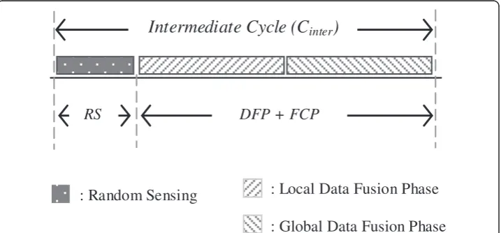
final clustering phase (FCP) are executed in parallel thereby performing better time utilization. The data aggregation or data fusion phase (DFP) is further classified in local and global phases respectively. The local DFP is carried out by individual nodes with the help of local probability measure and the global DFP is performed by the cluster heads using the global probability measure. Since, the aggregation process is involved only within the cluster, the FCP can continue in parallel (outside the clusters) without collision. This efficient utilization of time ultimately results in significant energy savings. In Figure 2, the working slots for intermediate cycles are highlighted. We assume that our cluster formation procedure is static, i.e. the sensors are stationery and are all assigned to a fixed cluster at the initiation of the network that remains unchanged over the entire lifetime of the sensor network. After the clusters are formed at the network start-up, the consecutive data cycles involve random sampling (or sensing) and data fusion process (local as well as global).
Simulation and performance evaluations
The simulation of the proposed clustering and entropy-based aggregation is performed using Network Simulator (NS-2) [29,30]. Moreover, on the basis of the tracing data
Intermediate Cycle (C
inter)
RS
DFP + FCP
: Local Data Fusion Phase
: Global Data Fusion Phase
: Random Sensing
Figure 2Network timeline diagram for the intermediate cycles. Initial Cycle (Cinitial)
RS PCP DFP + FCP
: Local Data Fusion Phase
: Global Data Fusion Phase
: Final Clustering Phase : Random Sensing
: Preliminary Clustering Phase
generated in NS-2 and other log files, the graphical evaluation is generated using
MATLAB [31]. In our simulation, the sensor nodes are randomly deployed over a
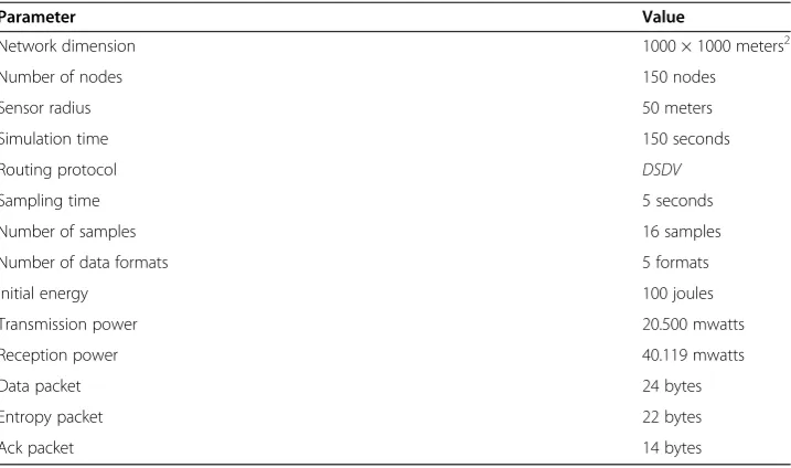
network of dimension 1000 x 1000 square meters. Our proposed clustering method uses divergence measure to discover clusters in the network. The simulation parameters used for the experimentation are specified in Table 1.
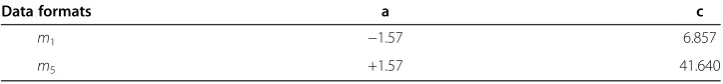
We have used Gaussian Bell and Sigma membership functions to monitor the fuzzy environmental parameter (temperature). The simulation parameters of the membership functions are provided in Table 2 and Table 3 respectively. The trend of the membership function, over the range of temperature being monitored, is highlighted in Figure 3.
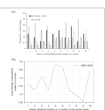
The clustered nodes keep track of the frequency of data formats sensed during the sampling period. The bar graph plotted in Figure 4 displays the variation of local probability of different data formats with respect to a randomly chosen cluster in the sensor network. Figure 4(a) represents the local entropy sent by the sensors to its CH. It is evident from the graph that node with id 5 gives highest entropy owing to the least variation of the same node in Figure 4(b). Therefore the fact that, least divergence is the implication of maximum entropy is verified.
Figure 5 provides an estimation of the number of aggregation cycles performed with 50, 100 and 150 nodes for a given amount of energy (in joules). The elevation in the trend apparently shows that the increase in number of aggregated samples is achieved at the minor cost of minimum packets transmission. Also, it is apparent that as the number of sensors rises from 50 to 150, the graph upraises specifying greater aggregation cycles. Moreover, the drift becomes smoother for 150 nodes, which implies that the performance of our protocol improves with increasing number of sensor nodes. This behavior is explained by the increase in the density of nodes ensures better exploitation of spatial property (of data sampled by different sensors).
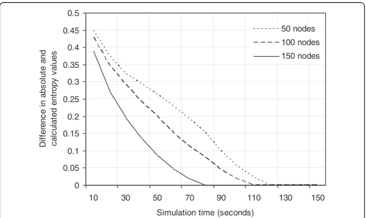
Figure 6 shows the convergence rate of calculated entropy with absolute entropic value. It can be seen that on average the proposed algorithm performs in good conjunction with the absolute value. However, for lesser number of sensor nodes (50 nodes), the trend stagnates in the early simulation phase. The reason is reduced accuracy in sampled data
Table 1 Simulation parameters used for performance evaluation
Parameter Value
Network dimension 1000 × 1000 meters2
Number of nodes 150 nodes
Sensor radius 50 meters
Simulation time 150 seconds
Routing protocol DSDV
Sampling time 5 seconds
Number of samples 16 samples
Number of data formats 5 formats
Initial energy 100 joules
Transmission power 20.500 mwatts
Reception power 40.119 mwatts
Data packet 24 bytes
Entropy packet 22 bytes
because of lesser utilization of spatio-temporal correlation. With increased node deployment, the convergence improves. This proves that our theoretical aggregation model results in good performance on implementation.
The graph presented in Figure 7 shows the average transmission cost contributed by our proposed Divergence Measure based Clustering (DMC) + Entropy based Data Aggregation (EDA) along with Hybrid Energy-Efficient Distributed Clustering (HEED) and Belief Propagation (BP) [10,11]. The maximum message size of BP is 74 bytes which are forwarded frequently in the network for the purpose of updation of local belief by individual nodes. As a result of which we find degradation in the performance of BP at the beginning of simulation period. Though BP performs lesser re-clustering than HEED, but owing to the smaller size of the messages in HEED (29 bytes) it achieves eventually better results in the late simulation period. However, our proposed DMC+EDA protocol presents best results than its comparatives. The graph, however, elevates slightly during the period of 50-90 seconds to compensate for the initial cluster formation. The clusters constructed using divergence measure exhibit comparatively better stability during the course of simulation. Moreover, the packet size of our protocol is maximum 24 bytes (minimum size being 14 bytes) which reduces the transmission cost to a greater extent.
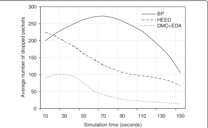
Figure 8 compares the average number of packets dropped by all the protocols respectively. As a matter of fact, HEED triggers more clustering processes than BP. Consequently, in case of HEED the nodes die out at a quicker rate. As a result, with fewer alive nodes the number of cluster heads tends to increase rapidly. This increases number of transmissions and therefore the chances of packet drops. However, due to rapid energy exhaustion the packet drop rate falls in the later simulation course. This is apparent from the HEED graph that steeps down towards the end of simulation. For BP the graph shows stability in clustering process resulting in better aggregation, lesser transmissions and reduced packet loss. But, owing to high transmission cost, BP finally deteriorates in the later simulation phase. Above all, our proposed scheme illustrates perfect combination of clustering and data aggregation over the entire simulation process. Increase in packet loss occurs at the network startup due to primary cluster formation. Once the network stabilizes, the outcome trend also becomes persistent.
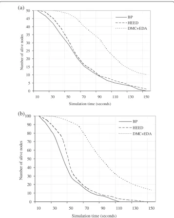
Finally, in Figure 9, the results of network lifetime is plotted for our protocol in association with its comparatives for varying number of nodes, 50 (Figure 9a) and
Table 3 SIGMF parameters table
Data formats a c
m1 −1.57 6.857
m5 +1.57 41.640
Table 2 GBELLMF parameters table
Data formats a b c
m2 2.86 2.43 12.60
m3 4.10 3.86 24.36
1.35 1.4 1.45 1.5 1.55 1.6
1 2 3 4 5 6 7 8 9 10
Nodes reporting entropy in a cluster to the cluster head
Loc
a
l ent
ropy
c
o
m
put
ed by
nodes
i
n
a c
lus
te
r
DMC+EDA
0 0.1 0.2 0.3 0.4 0.5 0.6
1 2 3 4 5 6 7 8 9 10
Nodes sensing different data formats in a cluster
P
ro
b
ab
ility
o
f d
ata
f
o
rm
at
s
c
m1 m2 m3 m4 m5
(a)
(b)
Figure 4a. Variation in probability of sensed data formats in a cluster. b. Local entropy sent by sensors to CH in a cluster.
0 5 10 15 20 25 30 35 40 45 50
0 0.1 0.2 0.3 0.4 0.5 0.6 0.7 0.8 0.9 1
Range of temperature monitored
V
a
lu
e
o
f m
e
m
b
e
rs
h
ip
fu
n
c
tio
n
cold normal hot very cold very hot
100 (Figure 9b) respectively. The lifetime performance of the protocols is illustrated in terms of remaining number of alive nodes. Evidently, our proposed scheme achieves sig-nificant improvement during the simulation. It is worth revealing that the gain in lifetime is achieved by sending the entropy of nodes in the first phase of aggregation followed by reduced data transmission (expected value) in second phase. This results in reducing the bulk of packets transfer, thereby increasing the network lifetime commendably. Moreover, as the number of initially deployed nodes is increased to 100, HEED and BP fails to keep the network functional till the end of simulation period (Figure 9b).
0 0.05 0.1 0.15 0.2 0.25 0.3 0.35 0.4 0.45 0.5
10 30 50 70 90 110 130 150
Simulation time (seconds)
D
if
fe
renc
e i
n
abs
ol
ut
e and
c
a
lc
ul
at
ed ent
ro
py
v
a
lues
50 nodes 100 nodes 150 nodes
Figure 6Convergence rate analysis of absolute and calculated entropy.
0 10 20 30 40 50 60 70 80 90 100
5 15 25 35 45 55 65 75 85 95
Initial sensor energy (joules)
d
e
mr
ofr
e
p
s
el
c
y
c
n
oit
a
g
er
g
g
a
f
o
r
e
b
m
u
N
50 nodes 100 nodes
150 nodes
Hence, the above experimental results rationalize the development of our proposed clustering and aggregation strategy.
Conclusion & future research directions
In this research, we have demonstrated that our proposed clustering protocol in wire-less sensor network provides significant energy savings. The clustering process is purely distributed and is based on the sensed data, regardless of geographic positioning and distance measures. We have calculated the precision of sensor data on the basis of local and global probability model. Furthermore, we have also analyzed the rate and impact
0 50 100 150 200 250 300
10 30 50 70 90 110 130 150
Simulation time (seconds)
st
e
k
c
a
p
d
e
p
p
or
d
f
o
r
e
b
m
u
n
e
g
ar
e
v
A
BP HEED DMC+EDA
Figure 8Evaluating average number of dropped packets for BP, HEED and DMC+EDA protocols.
0 500 1000 1500 2000 2500 3000 3500 4000 4500
10 30 50 70 90 110 130 150
Simulation time (seconds)
)
s
et
y
b(
t
s
o
c
n
oi
s
si
m
s
n
art
e
g
ar
e
v
A
BP HEED DMC+EDA
of information gain, i.e. convergence rate of calculated sensor entropy towards the absolute value. We have also defined the working slots to aggregate data for the initial period with partially clustered network and for the intermediate cycles, once the whole network is clustered.
The simulations of our proposed methods have shown outperforming results. The entropy measurement facilitates the efficient selection of maximum information bearing nodes, which further makes more accurate aggregation at the cluster head. It is also clarified that our proposed data aggregation technique performs in energy efficient manner. Moreover, the energy consumption in the network has also been carried out for several aggregation cycles. Therefore, it can be concluded that
0 5 10 15 20 25 30 35 40 45 50
10 30 50 70 90 110 130 150
Simulation time (seconds)
N
u
m
b
er
of
al
iv
e nodes
BP HEED DMC+EDA
0 10 20 30 40 50 60 70 80 90 100
10 30 50 70 90 110 130 150
Simulation time (seconds)
N
u
m
b
er
of
al
iv
e nodes
BP
HEED DMC+EDA
(a)
(b)
entropy based fusion is relevant in terms of information integrity, network lifetime as well as energy utilization.
Thus far we have concentrated on the homogeneous sensor networks with a single powerful processing center (sink). In our future work, we would rather focus on the heterogeneous wireless sensor networks with multiple resource-rich actors for carrying out energy consuming tasks. Apart from this, we would emphasis our effort on developing novel entropy-based techniques so as to enrich the integrity of aggregated content, thereby maintaining a delay constrain on the computational efficiency.
Competing interest
Both authors declare that they have no competing interests.
Authors’contributions
The authors have performed entropy based data aggregation that is computed from the proposed local and global probability distribution models, for extracting high precision data from the sensor nodes. An energy efficient clustering method is also proposed with the help of cluster divergence measure. Experimental analysis is carried out in terms of convergence rate, aggregation cycles, average packet drops, transmission cost and network lifetime. Both authors read and approved the final manuscript.
Authors’information
Adwitiya Sinha has completed Bachelor of Computer Applications and Master of Computer Applications in 2006 and 2008. She received Master of Technology in the Computer Science and Technology in 2010 from Jawaharlal Nehru University, New Delhi, India. Presently, she is working towards her PhD in the same university. She is the recipient of Senior Research Fellowship from Council of Scientific and Industrial Research, India. Her major interest lies in energy-efficient wireless networking, mobile and ad hoc communication, data aggregation and filtration techniques. D. K. Lobiyal received his Bachelor of Technology in Computer Science from Lucknow University, India. He received Master of Technology and PhD both in Computer Science from Jawaharlal Nehru University, New Delhi, India. Presently, he is working as an Associate Professor in the School of Computer and Systems Sciences at Jawaharlal Nehru University. His areas of research interest are Wireless ad Hoc Networks, Video on Demand, and Natural Language Processing (NLP).
Received: 1 February 2013 Accepted: 29 July 2013 Published: 9 August 2013
References
1. Akyildiz IF, Su W, Sankarasubramaniam Y, Cayirci E (2002) Wireless sensor networks: a survey. J Comp Networks 38(4):393–422, Elsevier
2. Yong-Min L, Shu-Ci W, Xiao-Hong N (2009) The architecture and characteristics of wireless sensor networks. IEEE Int Conf Comp Technol Dev 1:561–565, 13-15 November 2009
3. Potdar V, Sharif A, Chang E (2009) Wireless sensor networks: a survey. IEEE Int Conf Adv Inf Netw Appl:636–641, 26-29 May 2009
4. Eskandari Z, Yaghmaee MH, Mohajerzadeh AH (2008) Energy efficient spanning tree for data aggregation in wireless sensor networks. IEEE Proceedings of 17th International Conference on Computer Communications and Networks., pp 1–5, 3-7 August 2008
5. Galluccio L, Palazzo S, Campbell AT (2008) Efficient data aggregation in wireless sensor networks: an entropy-driven analysis. IEEE 19th International Symposium on Personal, Indoor and Mobile Radio Communications., pp 1–6, 15-18 September 2008
6. Cai W, Zhang M (2008) Data aggregation mechanism based on wavelet-entropy for wireless sensor networks. 4th IEEE International Conference on Wireless Communications, Networking and Mobile Computing, pp 1–4, 12-14 October 2008
7. Heinzelman WR, Chandrakasan A, Balakrishnan H (2000) Energy-efficient communication protocols for wireless microsensor networks. IEEE Proceedings of the 33rd Hawaii International Conference on System Sciences, pp 1–10, 4-7 January 2000
8. Yu B, Li J, Li Y (2009) Distributed data aggregation scheduling in wireless sensor networks. IEEE INFOCOM:2159–2167, 19-25 April 2009
9. Azim MA, Moad S, Bouadallah N (2010) SAG: Smart Aggregation Technique for continuous-monitoring in wireless sensor networks. IEEE International Conference on Communications, pp 1–6, 23-27 May 2010
10. Jiang H, Jin S, Wang C (2010) Parameter-based data aggregation for statistical information extraction in wireless sensor networks. IEEE Trans Vehicular Technol 59(8):3992–4001
11. Ma Y, Guo Y, Tian X, Ghanem M (2011) Distributed clustering-based aggregation algorithm for spatial correlated sensor networks. IEEE Sensors Journal 11(3):641–648
12. Tsai YR, Chang CJ (2011) Cooperative information aggregation for distributed estimation in wireless sensor networks. IEEE Trans Signal Processing 8:3876–3888
13. Younis O, Fahmy S (2004) Distributed clustering in Ad-hoc sensor networks: a hybrid, energy-efficient approach. IEEE INFOCOM:1–12, 7-11 March 2004
15. Chitnis L, Dobra A, Ranka S (2008) Aggregation methods for large-scale sensor networks. ACM Trans Sensor Netw 4(2):1–36
16. Castelluccia C, Chan AC-F, Mykletun E, Tsudik G (2009) Efficient and provably secure aggregation of encrypted data in wireless sensor networks. ACM Trans Sensor Netw 5(3):1–36
17. Xiong N, Svensson P (2002) Multi-sensor management for information fusion: issues and approaches. Inf Fusion 3(2):163–186, Elsevier
18. Heinzelman W, Chandrakasan A, Balakrishnan H (2002) An application-specific protocol architectures for wireless microsensor networks. IEEE Trans Wireless Comm 1(4):660–670
19. Ghiasi S, Srivastava A, Yang XJ, Sarrafzadeh M (2004) Optimal energy aware clustering in sensor networks. Sensors J 2(7):258–269
20. Srinivasan SM, Azadmanesh A (2008) Data aggregation in static Adhoc networks, 3rd IEEE international conference on industrial and information systems., pp 1–6, 8-10 December 2008
21. Wang X, Li J (2009) Precision constraint data aggregation for dynamic cluster-based wireless sensor networks. 5th International Conference on Mobile Ad-hoc and Sensor Networks., pp 172–179, 14-16 December 2009
22. Zhao F, Shin J, Reich J (2002) Information-driven dynamic sensor collaboration. IEEE Signal Process Mag 19:61–72 23. Commuri S, Tadigotla V (2007) Dynamic data aggregation in wireless sensor networks, IEEE 22nd International
Symposium on Intelligent Control., pp 1–6, 1-3 October 2007
24. Kong L, Chen Z, Yin F (2007) Optimum design of a window function based on the small-world networks. IEEE International Conference on Granular Computing, p 97, 2-4 November 2007
25. Eguchi S, Copus J (2006) Interpreting Kullback–Leibler Divergence with the Neyman–Pearson Lemma. J Multivar Anal 97:2034–2040, Elsevier
26. Chang H, Yao Y, Koschan A, Abidi B, Abidi M (2009) Improving face recognition via narrowband spectral range selection using Jeffrey Divergence. IEEE Trans Inf Forensics Security 4(1):111–123
27. Duch W (2004) Uncertainty of data, Fuzzy membership functions, and multi-layer perceptrons. IEEE Trans Neural Netw 20:1–12
28. Gray RM (1990) Entropy and information theory. Springer-Verlag, New York, USA 29. Fall K, Varadhan K (2009) The ns manual, the VINT project
30. Altman E, Jemenez T (2003) NS simulator for beginners. Morgan & Claypool Publishers, Florida, USA 31. Attaway S (2009) Part I: programming and problem solving using MATLAB, in: MATLAB-A Practical Approach.
Elsevier, USA, pp 1–196
doi:10.1186/2192-1962-3-13
Cite this article as:Sinha and Lobiyal:Performance evaluation of data aggregation for cluster-based wireless sensor network.Human-centric Computing and Information Sciences20133:13.
Submit your manuscript to a
journal and benefi t from:
7Convenient online submission
7Rigorous peer review
7Immediate publication on acceptance
7Open access: articles freely available online
7High visibility within the fi eld
7Retaining the copyright to your article