R E S E A R C H
Open Access
Referenceless image quality assessment
by saliency, color-texture energy, and gradient
boosting machines
Pedro Garcia Freitas
1*, Welington Y. L. Akamine
2and Mylène C. Q. Farias
2Abstract
In most practical multimedia applications, processes are used to manipulate the image content. These processes include compression, transmission, or restoration techniques, which often create distortions that may be visible to human subjects. The design of algorithms that can estimate the visual similarity between a distorted image and its non-distorted version, as perceived by a human viewer, can lead to significant improvements in these processes. Therefore, over the last decades, researchers have been developing quality metrics (i.e., algorithms) that estimate the quality of images in multimedia applications. These metrics can make use of either the full pristine content (full-reference metrics) or only of the distorted image (referenceless metric). This paper introduces a novel referenceless image quality assessment (RIQA) metric, which provides significant improvements when compared to other state-of-the-art methods. The proposed method combines statistics of the opposite color local variance pattern (OC-LVP) descriptor with statistics of the opposite color local salient pattern (OC-LSP) descriptor. Both OC-LVP and OC-LSP descriptors, which are proposed in this paper, are extensions of the opposite color local binary pattern (OC-LBP) operator. Statistics of these operators generate features that are mapped into subjective quality scores using a machine-learning
approach. Specifically, to fit a predictive model, features are used as input to a gradient boosting machine (GBM). Results show that the proposed method is robust and accurate, outperforming other state-of-the-art RIQA methods.
Keywords: Color-texture analysis, Gradient boosting machine, Local variance patterns, Local salient patterns, Referenceless image quality assessment, Regression, Visual attention
Background
The rapid growth of current multimedia industry, and the consequent increase in content quality requirements, have prompted the interest in visual quality assessment methodologies [1]. Because most multimedia applications are designed for human observers, visual perception has to be considered when measuring visual quality [2]. Psy-chophysical experiments (or subjective quality assessment methods) performed with human subjects are consid-ered the most accurate methods to assess visual qual-ity [3]. However, these subjective methods are costly, time-consuming, and, for this reason, not adequate for real-time multimedia applications.
*Correspondence:[email protected]
1Department of Computer Science, University of Brasília, Campus Universitário Darcy Ribeiro, Brasília - DF 70919-970 Brazil
Full list of author information is available at the end of the article
Objective quality assessment metrics predict visual quality employing mathematical methods instead of human subjects. For instance, mean squared deviation (MSD) and peak-to-noise ratio (PSNR) are mathematical methods that can be used to measure the similarity of visual signals. However, MSD and PSNR scores often do not correlate well with the image quality as perceive by human observers (i.e., subjective scores) [4]. It is worth mentioning that, for an objective metric to be used in mul-timedia applications, its estimates must be well correlated with quality scores available in publicly available quality databases, which use standardized experimental proce-dures to measure the quality of a comprehensive series of visual signals.
Metrics can be classified according to the quantity of reference information (pristine content) required by the method. While full-reference (FR) metrics require the original content, reduced-reference (RR) metrics demand
papers of Fang et al. [6], Bahrami and Kot [7], Golestaneh and Chandler [8], and Li et al. [9–11]. These methods make assumptions about the type of distortion present in the signal and, as a consequence, have limited applications in more diverse multimedia scenarios.
Non-distortion-specific (NDS) methods, which do not demand a prior knowledge about the type of distortions in the signal, are more suitable for diverse multimedia sce-narios. In this case, instead of making assumptions about the main characteristics of specific distortions, the meth-ods make assumptions about the image characteristics. For instance, to find the relationship between gradient information and image quality, Liu et al. [12] and Li et al. [13] make assumptions about the image structure of reference images in the gradient domain. Some meth-ods compare the statistics of impaired and non-impaired (natural) images using a “natural scene statistic” (NSS) approach [14,15].
In addition to the aforementioned approaches, IQA methods can be classified as feature-based or human visual system (HVS)-based approaches. Feature-based approaches extract and analyze features from image sig-nals to estimate quality. Usually, these approaches require three steps. In the first step, descriptive features are extracted. Then, the extracted features are pooled to pro-duce a quality-aware feature vector. Finally, a model maps the pooled data into a numerical value that represents the quality score of the image under test. One example of a feature-based metric is the work of Mittal et al. [16], which is a spatial-domain method based on the NSS. Saad et al. [14,17] proposed another feature-based NSS method that operates in the discrete cosine transform (DCT) domain. Finally, Liu et al. [18] proposed a feature-based method that is based on spatial and spectral image entropies. More recently, some works proposed feature extraction used texture information to estimate image quality [19–27].
Instead of extracting basic features from images, HVS-based approaches aim to mimic the HVS behavior. Hith-erto, various HVS properties have been used in quality metrics, including structural information [28, 29] and error and brightness sensitivities [30,31]. The acclaimed structural similarity index (SSIM) [32] is based on the assumption that HVS is more sensitive to the structural
been proposed [35–37]. These CNN-based methods are established on the comparison between the hierarchy of the human visual areas and the layers of a CNN [38,39].
In recent years, HVS-based image quality approaches that incorporate visual saliency models (VSM) have been a trend [40–43]. Image quality metrics and VSM are inherently correlated because both of them take into account how the HVS perceives the visual content (i.e., how humans perceive suprathreshold distortions) [42]. Since VSM provide a measurement of the region’s impor-tance, they can be successfully used for weight distor-tions in image quality algorithms. Several researchers have studied how the saliency information can be incor-porated into visual quality metrics to enhance their performance [41, 44–47]. However, most VSM-based quality metrics are FR approaches. Among the exist-ing VSM-based RIQA methods, most are DS methods that cannot be used as general-purpose RIQA methods (GP-RIQA).
Additionally, most of current GP-IQA methods have no good prediction accuracy for color and contrast-distorted images. For instance, Ortiz-Jaramill et al. [48] demon-strated that current color difference measures (i.e., FR-IQA methods that compute color differences between processed and reference images) present little correla-tion with subjective quality scores. Also, even though some DS-IQA methods are able to predict the quality of contrast-distorted images [49], most GP-IQA methods have a poor prediction performance. This low perfor-mance leads to authors often omitting the results for these types of image distortions [18,20,23,50].
saliency information using a VSM to weight the OC-LBP statistics. The OC-LVP descriptor uses concepts intro-duced by the local variant patterns (LVP) [52] to modify the OC-LBP and measure the color-texture energy. The method uses the statistics of OC-LVP and OC-LSP as input of a gradient boosting machine (GBM) [53,54] that learns the predictive quality model via regression. When compared to previous work [52], in this work, we use OC-LSP and OC-LVP operators, instead of the simpler LVP operator. The metric design of the metric was also modi-fied to use a GBM, instead of the random forest regression algorithm.
The rest of this paper is divided as follows. In the “A brief review of local binary patterns” section, the basis of texture analysis is revised. In the “Opponent color local binary pattern” section, the base color-texture descriptor is summarized. In the “Opponent color local salient pattern” and “Opposite color local variance pattern” sections, the proposed descriptors are detailed. In the “Feature extrac-tion” and “Gradient boosting machine for regression” sections, we describe how to use the proposed descriptors to predict image quality without references. An exten-sive analysis of the results is presented in the “Results and discussion” section. Finally, the “Conclusions” section concludes this paper.
Methods
In this section, we review the basic texture operator local binary pattern (LBP) and its improved color-texture extension, the opposite color local binary patterns (OC-LBP). Then, we describe the proposed quality-aware descriptor, named the color local salient patterns (OC-LSP) and the color local variance patterns (OC-LVP). Finally, this section finishes with the proposed quality assessment method based on these operators.
A brief review of local binary patterns
Local binary pattern (LBP) is indubitably one of the most effective texture descriptors available for texture analy-sis of digital images. It was first proposed by Ojala et al. [55] as a specific case of the texture spectrum model [56]. Being I ∈ Rm×n the image whose texture we want to describe, the ordinary LBP takes the form:
LBPR,P(Ic)= P−1
p=0
f Ip,Ic,p, (1)
where
fIp,Ic,p
=SIp−Ic
·2p (2) and
S(t)=
1, ift≥0,
0, otherwise. (3)
In Eq.1,Ic = I(x,y)is an arbitrary central pixel at the position (x,y) andIp = I(xp,yp) is a neighboring pixel surroundingIc, where:
xp=x+Rcos
2π· p
P
,
and
yp=y−Rsin
2π·p
P
.
In this case,Pis the number of neighboring pixels sam-pled from a distance ofRfromIctoIp. Figure1illustrates examples of symmetric samplings for different neighbor-ing points (P) and radius (R) values.
Figure2exemplifies the steps for applying the LBP oper-ator on a single pixel (Ic = 35), located in the center of a 3× 3 image block, as shown in the bottom-left of this figure. The numbers in the yellow squares of the block represent the order in which the operator is com-puted (counter-clockwise direction starting from 0). In this figure, we use an unitary neighborhood radius (R=1) and eight neighboring pixels (P = 8). After calculating S(t) (see Eq.3) for each neighboring pixelIp, we obtain a binary output for each Ip (0 ≤ p ≤ 7), as illustrated in the block in the upper-left position of Fig. 2. In this block, black circles correspond to “0” and white circles to “1”. These binary outputs are stored in a binary for-mat, according to their position (yellow squares). Then, the resulting binary number is converted to the decimal format. For a complete image, we use the LBP operator to obtain a decimal number for each pixel of the image, by makingIcequal the current pixel.
When an image is rotated, Ip values move along the perimeter of the circumference (aroundIc), generating a
Fig. 2Pattern extraction process for a given pixel using LBP and LVP operators withR=1,P=8,Ic=35, andIp= {71, 32, 91, 103, 21, 10, 34, 13}
circular shift in the binary number generated. As a con-sequence, a different decimalLBPR,P(Ic)value is obtained. To remove this effect, we assign a unique identifier to each rotation, generating a rotation invariant LBP:
LBPriR,P(Ic)=min
ROTRLBPR,P(Ic),k , (4)
wherek= {0, 1, 2,· · ·,P−1}andROTR(x,k)is the circu-lar bit-wise right shift operator that shifts the t-uplexby movingkpositions.
Due to the primitive quantization of the angular space [57,58],LBPR,PandLBPriR,P operators do not always pro-vide a good discrimination [58]. To improve the discrim-inability of the LBP operator, Ojala et al. [55] proposed an improved operator that captures fundamental pattern properties. These fundamental patterns are called “uni-form” and computed as follows:
LBPuR,P(Ic)=
⎧ ⎨ ⎩
P−1
p=0
fIp,Ic,p
ULBPriR,P≤2,
P+1 otherwise,
(5)
whereU(LBPP,R)is the uniform pattern given by:
U(LBPP,R)= (IP−1,I0)+ P−1
p=1
Ip,Ip−1
, (6)
and
Ix,Iy
= |S(Ix−Ic)−S(Iy−Ic)|. (7) In addition to a better discriminability, the uniform LBP operator (Eq.5) has the advantage of generating fewer dis-tinct LBP labels. While the “nonuniform” operator (Eq.1) produces 2P different output values, the uniform opera-tor produces only P+2 distinct output values, and the “rotation invariant” operator producesP(P−1)+2 points. Opponent color local binary pattern
The LBP operator is designed to characterize texture of grayscale images. Although this restriction may not affect
many applications, it may be unfavorable for image qual-ity assessment purposes because LBP is not sensitive to some types of impairments, such as contrast distortions or chromatic aberrations. As pointed out by Maenpaa et al. [51], texture and color have interdependent roles. When luminance-based texture descriptors (e.g., LBP) achieve good results, color descriptors can also obtain good results. However, when color descriptors are unsuc-cessful, luminance texture descriptors can still present a good performance. For this reason, operators that inte-grate both color and texture information tend to be more successful to predict the quality of images with a wider range of distortions.
In order to integrate color and texture into a single descriptor, Maenpaa et al. [51] introduced the opponent color local binary pattern (OC-LBP). The OC-LBP extends the LBP operator by incorporating color information, while keeping texture information. This color-texture descriptor is an extension of the operator proposed by Jain and Healey [59], which replaces the Gabor’s filtering with a variant of the LBP-inspired operator.
The OC-LBP descriptor operates on intra-channel and inter-channel color dimensions. In the intra-channel oper-ation, the LBP operator is applied individually, on each color channel, instead of being applied only on a sin-gle luminance channel. This approach is called “intra-channel” because the central pixel and the corresponding sampled neighboring points belong to the same color channels.
In the “inter-channel” operation, the central pixel belongs to a color channel and its corresponding neigh-boring points are necessarily sampled from another color channel. Therefore, for a three-channel color space, such as HSV, there are six possible combinations of chan-nels: OC-LBPHS, OC-LBPSH, OC-LBPHV, OC-LBPVH, OC-LBPSV, and OC-LBPVS.
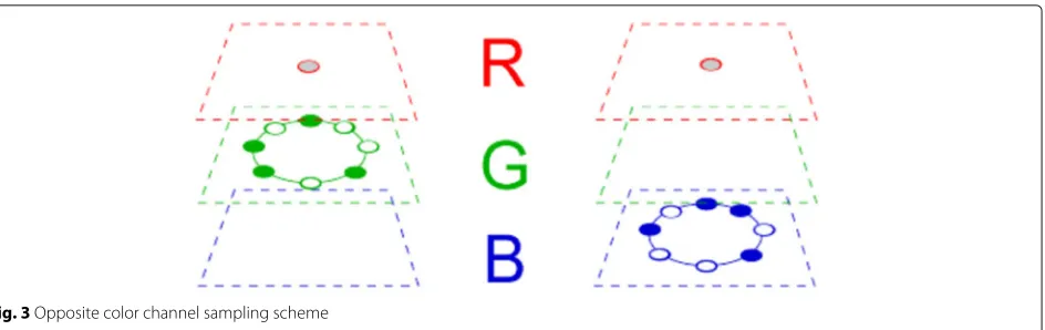
Fig. 3Opposite color channel sampling scheme
RGB image. From this figure, we can notice that two com-binations are possible: OC-LBPRG (left) and OC-LBPRB (right). In OC-LBPRG, the gray circle in the red channel is the central point, while the green circles in the green channel correspond to “0” sampling points and the white circles correspond to “1” sampling points, respectively. Similarly, in OC-LBPRB, the blue circles correspond to “0” sampling points and the white circles correspond to “1” sampling points, respectively.
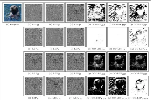
After computing the OC-LBP operator for all pixels of a given image, a total of six texture maps are generated. As depicted in Fig.4, three intra-maps and three inter-maps are generated for each color space. Although all possi-ble combinations of the opposite color channels allow six distinct maps, we observed that the symmetric opposing pairs are very redundant (e.g., OC-LBPRG is equivalent to OC-LBPGR, OC-LBPHS is equivalent to OC-LBPSH, and so on). Due to this redundancy, only the three more descriptive inter-maps are used.
Opponent color local salient pattern
Although OC-LBP increases the discriminability of LBP by incorporating color-texture information, it does not necessarily mimics the human visual system (HVS) behavior. To generate general-purpose descriptors that incorporates visual attention, we modify the OC-LBP by incorporating the VS information. The modified descriptor is named opponent color local salient pattern (OC-LSP). Basically, we compute the OC-LBP for all pixels of an image, obtaining the intra- and inter-channel maps of the image (see Fig.4). In other words, beingL∈
{LBPX, LBPY, LBPZ, OC-LBPXY, OC-LBPXZ, OC-LBPYZ}, where XYZ represents any color space (i.e., HSV, CIE Lab, RGB, and YCbCr) normalized in the range [0, 255]. Each labelL(x,y)corresponds to the local texture asso-ciated to the pixel I(x,y). We use a VSM to generate a saliency map W, where each pixel W(x,y) corre-sponds to the saliency of pixel I(x,y). Figure 5a and h
depicts an image and its corresponding saliency map, respectively.
The saliency mapWis used to weight each pixel of the mapL. This weighting process is used to generate a fea-ture vector based on the histogram ofLweighted byW. The histogram is given by the following expression:
H= {h0,h1,h2,· · ·,hP+1}, (8) wherehφ is the count of the labelL(x,y)weighted byW, as given by:
hφ =
x,y
W(x,y)·δ(L(x,y),φ), (9)
where
δ(v,u)=
1, ifv=u,
0, otherwise. (10)
The number of bins ofHis the number of distinct labels ofL. Therefore, we can remap eachL(x,y)to its weighted form, generating the mapS(x,y)that is the local salient pattern (LSP) map. Figure5depictsS.
Opposite color local variance pattern
The use of the LBP operator (or of its variants) in IQA is based on the assumption that visual distortions affect image textures and their statistics. Particularly, images with similar distortions, at similar strengths, have tex-tures that share analogous statistical properties. Recently, Freitas et al. [52] used a second assumption, which con-siders the changes in the spread of the local texture energy that are commonly observed in impaired images. For instance, a Gaussian blur impairment decreases the local texture energy, while a white noise impairment increases it. Therefore, we can use techniques that measure texture energy in RIQA algorithms.
Fig. 4Original image and its output maps, computed using the OC-LBP descriptor computed in HSV (b–g), Lab (h–m), RGB (n–s), and YCbCr (t–y) color spaces
The LVP descriptor computes the local texture-energy according to the following formula:
LVPuR,P(Ic)=
P·VR,P(Ic)−
LBPuR,P(Ic)
2
P2
, (11)
where:
VR,P(Ic)= P−1
p=0
f(tp,tc,p)
2
, (12)
and·represents the operation of rounding to the nearest integer.
Figure2depicts the steps to extract the texture-energy information using the LVP operator. Similar to LBP oper-ator, a LVP map is generated after computing the LVP descriptor for all pixels of a given image. A compari-son between LVP and LBP maps is depicted in Fig. 6. In this figure, the first column corresponds to the refer-ence (undistorted) image, while the three other columns correspond to images impaired with blur, white noise, and JPEG-2K distortions. The first row shows the col-ored images, while the second and third rows show the corresponding LBP and LVP maps, respectively. Notice
that textures are affected differently by different impair-ments. For instance, the LBP maps (second line of Fig.6) corresponding to noise, blurry, and JPEG-2K com-pressed images have clear differences among themselves. However, the LBP map corresponding to the noise and reference images are similar. This similarity affects the discrimination between unimpaired and impaired images, affecting the quality prediction. On the other hand, the LVP channels (third line of Fig.6) clearly show the differ-ences between impaired and reference images.
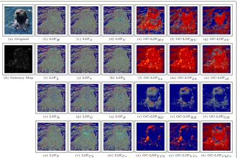
Fig. 5Original image (a), its saliency (h), and its output maps, computed using the OC-LSP descriptor computed in HSV (b–g), Lab (i–n), RGB (o–t), and YCbCr (u–z) color spaces
the central point in a channel and the neighboring points in another channel (across channels).
Feature extraction
The proposed RIQA method uses a supervised ML approach. The set of features is extracted, as depicted in Fig.8. The first step of the feature extraction process consists of splitting the color channels. Using the indi-vidual color channels, we compute the OC-LSP maps. In Fig.5, we observe that, independent of the color space,
the intra-channel maps are very similar. This similarity and the invariance between color spaces indicate that intra-channel statistics do not depend on the chosen color space.
The inter-channel maps, on the other hand, are not sim-ilar to each other. Moreover, they show considerable dif-ferences for the different color spaces. This indicates that different OC-LSP are able to extract different information, depending of the color space. Therefore, based on these observations, we use Eq. 8 to compute the histograms
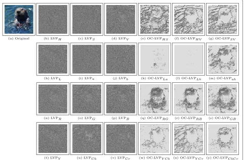
Fig. 7Original image and its output maps, computed using the OC-LVP descriptor computed in HSV (b–g), Lab (h–m), RGB (n–s), and YCbCr (t–y) color spaces
H of LSPH, OC-LSPHS, OC-LSPHV, OC-LSPSV, OC-LSPLa, OC-LSPLb, OC-LSPab, OC-LSPRG, OC-LSPRB, OC-LSPGB, OC-LSPYCb, OC-LSPYCr, and OC-LSPCbCr maps. The concatenation of these histograms generates the OC-LSP feature set.
Finally, the OC-LVP feature set is generated by comput-ing the mean, variance, skewness, kurtosis, and entropy of each map, as depicted in Fig.8. The concatenation of OC-LVP and OC-LSP feature sets generates the feature vectorx, which is used as input to a regression algorithm.
Gradient boosting machine for regression
After concatenating the OC-LVP and OC-LSP feature sets to generate the feature vector x, we use it to pre-dict image quality. The prepre-diction is computed using x as input to a gradient boosting machine (GBM). GBMs are a group of powerful ML techniques that have shown substantial success in a wide range of practical appli-cations [53, 54]. In our application, we use a GBM regression model to map x to the database subjective scores.
Results and discussion
In this section, we analyze the proposed method by comparing it with some of the state-of-the-art methods. Specifically, this section describes the experimental setup and configurations used in the analysis of the impact of the color space on the performance of the proposed method and in the comparisons between the proposed method and available state-of-the-art methods.
Experimental setup
There are a number of existing benchmark image quality databases. In this work, we use the following databases:
• Laboratory for Image and Video Engineering (LIVE) Image Database version 2 [60]: The database presents 982 test images, including 29 originals and 5
categories of distortions. These images are in uncompressed BMP format at several dimensions, including 480×720, 610×488, 618×453, 627×482, 632×505, 634×438, 634×505, 640×512, and 768×512. The distortions include JPEG, JPEG 2000 (JPEG2k), white noise (WN), Gaussian blur (GB), and fast fading (FF).
• Computational and Subjective Image Quality (CSIQ) Database [28]: The database contains 30 reference images, obtained from public-domain sources, and 6 categories of distortions. These images are in 512×512×24 compressed bitmap (BMP) format (PNG image data). The distortions include JPEG, JPEG 2000 (JPEG2k), white noise (WN), Gaussian blur (GB), global contrast decrements (CD), and additive Gaussian pink noise (PN). In total, there are 866 distorted images.
• Tampere Image Database 2013 (TID2013) [61]: The database has 25 reference images and 3,000 distorted images (25 reference images×24 types of
distortions×5 levels of distortions). These images are in 512×384×24 uncompressed BMP format. The distortions include additive Gaussian noise (AGN), additive noise in color components (ANCC), spatially correlated noise (SCN), masked noise (MN), high frequency noise (HFN), impulse noise (IN),
quantization noise (QN), Gaussian blur (GB), image denoising (ID), JPEG, JPEG2k, JPEG transmission errors (JPEG+TE), JPEG2k transmission errors (JPEG2k+TE), non eccentricity pattern noise (NEPN), local block-wise distortions (LBD), intensity shift (IS), contrast change (CC), change of color saturation (CCS), multiplicative Gaussian noise (MGN), comfort noise (CN), lossy compression (LC), image color quantization with dither (ICQ), chromatic aberration (CA), and sparse sampling and reconstruction (SSR).
The Boolean Map Saliency (BMS) is used as the VSM algorithm [62]. We compare the proposed method with
a set of publicly available methods. The chosen state-of-the-art RIQA methods are the following: Codebook Repre-sentation for No-Reference Image Assessment (CORNIA) [23], Curvlet-based Quality Assessment (CQA) [50], Spa-tial and Spectral Entropies Quality Assessment (SSEQ) [18], Blind/Referenceless Image Spatial Quality Evalua-tor (BRISQUE) [16], local ternary patterns (LTP) [20], and No-Reference Free Energy Principe Metric (NFERM) [33]. Additionally, we also compared the proposed algo-rithm with three well-established FR-IQA metrics, namely PSNR, structural similarity (SSIM) [32], and reduced-reference image quality metric for contrast change (RIQMC) [49].
The trained-based RIQA methods are performed using the same training-and-testing protocol. The protocol con-sists of splitting each single database into two content-independent subsets (i.e., one subset for training and another for testing). To avoid overtraining and, therefore, failing to predict quality for other contents, scenes in the testing subset are not present in the training subset, and vice-versa. Considering this constraint, 20% of images are randomly selected for testing and the remaining 80% are used for training. This 80-20 split, training, and testing procedure is a simulation. We performed each simulation 1000 times, and the mean correlation value is reported. To compare the predicted and subjective quality scores, three correlation metrics were used: Spearman rank order correlation coefficient (SROCC), Pearson linear correla-tion coefficient (LCC), and Kendall rank order correlacorrela-tion coefficient (KRCC).
It is worth pointing out that each simulation is per-formed using all distortions in training. When the prediction performance “per distortion” is reported, the predicted data for each distortion is generated using the trained data using all distortions for train-ing. For the training-based methods based on the sup-port vector regression (SVR) algorithm, the training and predicting steps are implemented using the Sklearn library [63]. The SVR metaparameters are found using exhaustive grid search methods provided by Sklearn’s API. The proposed method, on the other hand, uses GBM regression implemented with the XGBoost [64] library.
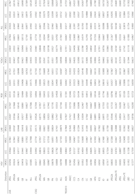
Impact of color space on prediction performance
To investigate the most suitable color space for the pro-posed method, we perform simulations with the LIVE2 database using the HSV, Lab, RGB, and YCbCr color spaces. For comparison proposes, we also tested the algorithm using the features obtained by combining all color spaces. Table1shows the average LCC, SROCC, and KRCC correlation scores (CS) for 1000 simulations.
JPEG2k 0.9309 0.9251 0.5795 0.8458 0.8405 0.8214 0.7302 0.8877 0.9223 0.8871
WN 0.9345 0.8761 0.4678 0.6931 0.6187 0.7276 0.7876 0.6454 0.9214 0.9346
GB 0.9358 0.9089 0.8007 0.8337 0.8526 0.7486 0.7766 0.9244 0.8962 0.9197
PN 0.9315 0.8871 0.3653 0.7740 0.5340 0.5463 0.6661 0.7828 0.6334 0.9461
CD 0.8862 0.8128 0.9565 0.4255 0.4458 0.5383 0.4172 0.2082 0.3774 0.8097
ALL 0.8088 0.8116 0.5066 0.7597 0.6969 0.6369 0.7007 0.8280 0.9142 0.8949
TID2013 AGC 0.8568 0.7912 0.3555 0.4166 0.2605 0.3964 0.3949 0.5963 0.7077 0.9217
AGN 0.9337 0.6421 0.6055 0.6416 0.5689 0.6051 0.6040 0.6631 0.8567 0.8662 CA 0.7759 0.7158 0.5726 0.7310 0.6844 0.4380 0.4366 0.6749 0.6357 0.5991
CC 0.4608 0.3477 0.8044 0.1849 0.1400 0.2043 0.2006 0.1886 0.2148 0.7583
CCS 0.6892 0.7641 0.0581 0.2715 0.2642 0.2461 0.2547 0.2384 0.3106 0.5765
CN 0.8838 0.6465 0.6262 0.2176 0.3553 0.1623 0.1642 0.3880 0.1385 0.5100 GB 0.8905 0.8196 0.7687 0.8063 0.8341 0.7019 0.7058 0.7465 0.8502 0.8655
HFN 0.9165 0.7962 0.4267 0.7103 0.7707 0.7104 0.7061 0.7626 0.8797 0.9319
ICQ 0.9087 0.7271 0.8691 0.7663 0.7044 0.6829 0.6834 0.7603 0.4804 0.7877 ID 0.9457 0.8327 0.8661 0.5243 0.7227 0.6711 0.6716 0.7063 0.6405 0.8388 IN 0.9263 0.8055 0.1222 0.6848 0.5874 0.4231 0.4272 0.6484 0.1735 0.6699
IS 0.7647 0.7411 0.5979 0.2224 0.2403 0.2011 0.2013 0.3291 0.0407 0.8792
JPEG 0.9252 0.8275 0.7293 0.7252 0.7815 0.6317 0.6284 0.6631 0.8711 0.6160
JPEGTE 0.7874 0.6144 0.6009 0.3581 0.5679 0.2221 0.2195 0.2314 0.1281 0.8531
JPEG2k 0.8934 0.7531 0.5967 0.7337 0.8089 0.7219 0.7205 0.7780 0.8068 0.3819
JPEG2kTE 0.8581 0.7067 0.7189 0.7277 0.6113 0.6529 0.6529 0.6594 0.1686 0.1754
LBD 0.1301 0.6213 0.2471 0.2833 0.2157 0.2382 0.2290 0.3813 0.1995 0.9000
LC 0.9386 0.8311 0.5346 0.5726 0.6682 0.4561 0.4460 0.6533 0.6516 0.7738 MGN 0.9085 0.7863 0.3751 0.5548 0.4393 0.4969 0.4897 0.6209 0.7159 0.1254
MN 0.8385 0.7388 0.0438 0.2650 0.2342 0.2506 0.2575 0.4243 0.2238 0.8769
NEPN 0.6931 0.5326 0.1496 0.1821 0.2855 0.1308 0.1275 0.1256 0.0667 0.1985
QN 0.8636 0.7428 0.8697 0.5383 0.4922 0.7242 0.7214 0.7361 0.7716 0.8662
SCN 0.9152 0.7934 0.7811 0.7238 0.7043 0.7121 0.7064 0.7015 0.2181 0.9146 SSR 0.9241 0.7774 0.6967 0.7101 0.8594 0.8115 0.8084 0.8457 0.7865 0.9023
ALL 0.6869 0.5758 0.4439 0.5416 0.6006 0.4925 0.4900 0.6078 0.3971 0.7231
Average 0.8377 0.7807 0.5808 0.6234 0.6262 0.5741 0.5893 0.6563 0.6084 0.7767
all distortions (23 out of 114 CS or 20.17%) and fol-lowed by Lab (13 out of 114 or 11.41%), HSV (10 out of 114 or 8.77%), and RGB (3 of 114 or 2.63%). However,
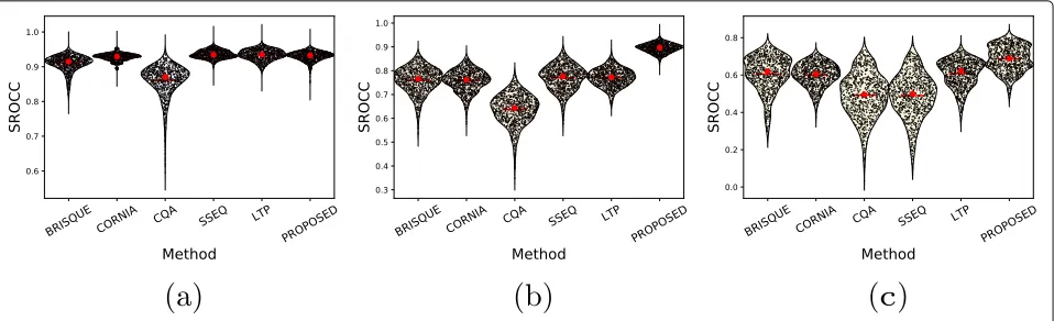
Fig. 9Bean plot of SROCC distributions from 1000 runs of simulations on tested databases.aLIVE.bCSIQ.cTID2013
Prediction performance using a single database
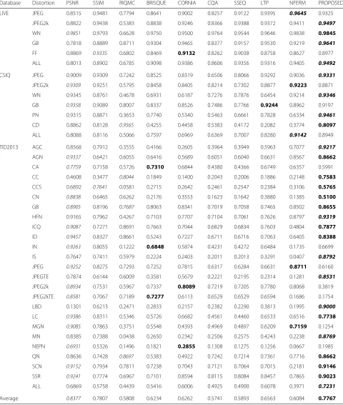
Table2 depicts the results for the tested methods using part of database for training and part for testing. Num-bers in italics represent the best correlation values among RIQA and FR-IQA methods, while numbers in bold corre-spond to the best correlation values considering only the RIQA methods.
From Table2, we can see that, for most databases, the proposed method achieves the best performance among the RIQA methods. For the LIVE2 database, the pro-posed method outperforms even the FR-IQA methods for JPEG2, WN, GB, and “ALL” distortions. For the PN and CD distortions of the CSIQ database, the proposed method provides a significantly better performance than the other RIQA methods. The only exception is RIQMC that obtained a mean SROCC of 0.9565, which is expected since it is a contrast-specific metric. The superior perfor-mance for PN distortions is probably due to the color-based features. The good performance for CD distortions is an important advantage of the proposed method, given that this distortion is a challenge for most RIQA methods. For the TID2013 database, the proposed method out-performs other RIQA methods for 18 out of the 25 distor-tions, followed by NFERM, BRISQUE, and CORNIA. For AGC, HFN, IS, JPEG+TE, SSR, LBP, and MN distortions, the performance of the proposed method surpasses even FR-IQA methods. The performance for AGC distortions is very good, similar to what was obtained for the PN dis-tortions of the CSIQ database. Albeit losing for RIQMC, which is a contrast-specific metric, the performance of the proposed method for CC and CD distortions of the CSIQ database is also good. This shows that the proposed method can handle contrast distortions.
Figure9depicts the distributions of the SROCC values computed between the subjective scores (MOS) and the predicted scores obtained using the tested RIQA meth-ods. The bean plots of this figure are generated using the distribution of SROCC values for the set containing all database distortions (corresponding to “ALL” in Table2).
From Fig.9a, we notice that almost all methods (with the exception CQA) present similar distributions of SROCC scores for the LIVE database. On the other hand, SROCC values vary more for CSIQ and TID2013 databases, as can be seen in Fig.9b,c.
Statistical difference significance test
We also conduct tests to determine the statistical signifi-cance of the differences of the coefficient values reported in Table 3. We used the Welch’s t test on the SROCC values corresponding to each color space, considering all distortions (“ALL” label), with a 95% confidence level. The cells in Table3 indicate whether the value of the corre-sponding row is statistically better (↑), statistically inferior (↓), or statistically equivalent () to the value of the cor-responding column. These results show that the proposed method has a statistically superior performance in all cases.
Performance for a cross-database validation
To investigate the generalization capability of the pro-posed method, we performed a cross-database validation. This validation consists of training the proposed RIQA method using all images of one database and testing them
Table 3Welch’sttest performed between SROCC average values for TID2013 database: “↑” indicates that the method depicted in the row is statistically superior to the one in the column, “↓” indicates that the row is worse than the column, and “” indicates that two methods have statistically the same performance
BRISQUE CORNIA CQA SSEQ LTP PROPOSED
BRISQUE – ↑ ↑ ↓
CORNIA – ↑ ↑ ↓ ↓
CQA – ↓ ↓
SSEQ – ↓ ↓
LTP – ↓
GB 0.8245 0.8133 0.8214 0.8624 0.8693 0.8693
ALL 0.7965 0.7599 0.8214 0.7955 0.8137 0.8923
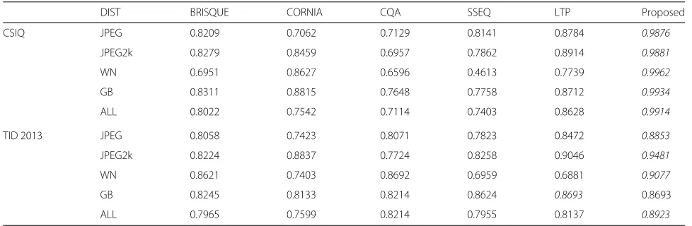
on the other databases. Table4depicts the SROCC val-ues obtained using LIVE as the training database and TID2013 and CSIQ as the testing databases. To perform a straightforward cross-database comparison, only simi-lar distortions were selected from each database. In other words, we select only JPEG, JPEG2k, WN, and GB dis-tortions of CSIQ since these disdis-tortions are also present in the training databases. The PN and CD distortions were removed from the test set and, therefore, they are not listed in Table 4. Likewise, for TID2013, only JPEG, JPEG2k, WN, and GB distortions were kept. In TID2013, the HFN distortion was chosen because it is the most similar to the WN distortion.
From Table4, we can notice that the proposed method outperforms the other RIQA methods for the cross-database validation test. Notice that the proposed method achieves the best performance for all cases, except for one. For TID, the proposed method outperforms the other methods for four out of the five distortions, while for CSIQ, it outperforms the other methods for all five distor-tions. Therefore, the cross-database validation test indi-cates that the proposed method has a better generalization capability, when compared to the tested state-of-the-art RIQA methods.
Conclusions
In this paper, we proposed a novel NDS-GP-RIQA method based on the statistics of two new texture descriptors: the OC-LSP and OC-LVP. OC-LSP descrip-tor extends the capabilities of the (previous) OC-LBP operator by incorporating texture, color, and saliency information. Similarly, OC-LVP fuses OC-LBP and LVP operators to incorporate texture, color, and energy infor-mation. Quality is predicted after training a regression model using a gradient boost machine. Experimental results showed that, when compared with state-of-the art RIQA methods, the proposed method has the best perfor-mance. More specifically, when considering a wide range
of distortions, the proposed method has a clear supe-riority. Since the proposed method is based on simple descriptors, it can be suitable for video quality assess-ment. Future works include a parallel implementation of the OC-LSP and OC-LVP descriptors.
Abbreviations
AGN: Additive gaussian noise; ANCC: Additive noise in color components; BMP: Bit map; BMS: Boolean Map Saliency; BRISQUE: Blind/referenceless image spatial quality evaluator; CA: Chromatic aberration; CC: Contrast change; CCS: Change of color saturation; CD: Contrast decrements; CN: Comfort noise; CNN: Convolutional neural networks; CORNIA: Codebook Representation for No-Reference Image Assessment; CQA: Curvlet-based quality assessment; CSIQ: Computational and subjective image quality; DCT: Discrete cosine transform; DS: Distortion-specific; FF: Fast fading; FR: Full-reference; FR-IQA: Full-reference image quality assessment; GB: Gaussian blur; GBM: Gradient boosting machine; GP: General-purpose; GP-IQA: General-purpose image quality assessment; GP-RIQA: General-purpose referenceless image quality assessment; HFN: High frequency noise; HSV: Hue, saturation, and value; HVS: Human visual system; ICQ: Image color quantization; ID: Image denoising; IN: Impulse noise; IQA: Image quality assessment; IS: Intensity shift; JPEG: Joint photographic experts group; JPEG+TE: JPEG transmission errors; JPEG2k: JPEG 2000; JPEG2k+TE: JPEG2k transmission errors; KRCC: Kendall rank order correlation coefficient; LBP: Local binary pattern; LBP: Local block-wise distortions; LC: Lossy compression; LCC: Linear correlation coefficient; LIVE: Laboratory for Image and Video Engineering; LTP: Local ternary patterns; LVP: Local variance pattern; MGN: Multiplicative Gaussian noise; ML: Machine learning; MN: Masked noise; MSD: Mean squared deviation; NDS: Non-distortion-specific; NDS-GP-RIQA: Non-distortion-specific general-purpose referenceless image quality assessment; NEPN: Non eccentricity pattern noise; NFERM: No-reference free energy principe metric; NSS: Natural scene statistic; OC-LBP: Opponent local binary patterns; OC-LSP: Opposite color local salient patterns; OC-LVP: Opposite color local variance patterns; PN: Pink noise; PNG: Portable network graphics; PSNR: Peak-to-noise ratio; QN: Quantization noise ; RGB: Red, green, and blue; RIQA: Referenceless image quality assessment; RIQMC: Reduced-reference image quality metric for contrast change; RR: Reduced-Reduced-reference; SCN: Spatially correlated noise; SROCC: Spearman rank order correlation coefficient; SSEQ: Spatial and spectral entropies quality assessment; SSIM: Structural similarity; SSR: Sparse sampling and reconstruction; SVR: Support vector regression; VSM: Visual saliency models; WN: White noise; YCbCr: Y luma component, color blue component relative to the green component, and color red component relative to the green component
Funding
Authors’ contributions
PGF wrote most of the text, figures, and analysis and developed the methods described in this manuscript. WYLA was responsible for implementing the compared methods to perform the experiments. MCQF is the principal investigator in this project and has guided the research and helped write and revise this manuscript. All authors read and approved the final manuscript.
Ethics approval and consent to participate Not applicable.
Competing interests
The authors declare that they have no competing interests.
Publisher’s Note
Springer Nature remains neutral with regard to jurisdictional claims in published maps and institutional affiliations.
Author details
1Department of Computer Science, University of Brasília, Campus Universitário Darcy Ribeiro, Brasília - DF 70919-970 Brazil.2Department of Electrical Engineering, University of Brasília, Campus Universitário Darcy Ribeiro, Brasília -DF 70919-970 Brazil.
Received: 4 March 2018 Accepted: 18 July 2018
References
1. Seshadrinathan K, Bovik AC (2011) Automatic prediction of perceptual quality of multimedia signals—a survey. Multimed Tools Appl 51(1):163–186
2. Chandler DM (2013) Seven challenges in image quality assessment: past, present, and future research. ISRN Signal Process, vol. 2013.https://doi. org/10.1155/2013/905685.https://www.hindawi.com/journals/isrn/2013/ 905685/
3. Telecom I (2000) Recommendation 500-10: Methodology for the subjective assessment of the quality of television pictures. ITU-R Rec. BT.500
4. Wang Z, Bovik AC (2009) Mean squared error: love it or leave it? A new look at signal fidelity measures. IEEE Signal Proc Mag 26(1):98–117 5. Moghadam A, Mohammadi P, Shirani S (2015) Subjective and objective
quality assessment of image: a survey. Majlesi J Electr Eng 9(1):55–83. https://profdoc.um.ac.ir/paper-abstract-1048833.html
6. Fang Y, Ma K, Wang Z, Lin W, Fang Z, Zhai G (2015) No-reference quality assessment of contrast-distorted images based on natural scene statistics. Signal Process Lett IEEE 22(7):838–842
7. Bahrami K, Kot AC (2014) A fast approach for no-reference image sharpness assessment based on maximum local variation. Signal Process Lett IEEE 21(6):751–755
8. Golestaneh SA, Chandler DM (2014) No-reference quality assessment of JPEG images via a quality relevance map. Signal Process Lett IEEE 21(2):155–158
9. Li L, Lin W, Zhu H (2014) Learning structural regularity for evaluating blocking artifacts in jpeg images. Signal Process Lett IEEE 21(8):918–922 10. Li L, Zhou Y, Lin W, Wu J, Zhang X, Chen B (2016) No-reference quality
assessment of deblocked images. Neurocomputing 177:572–584 11. Li L, Zhu H, Yang G, Qian J (2014) Referenceless measure of blocking
artifacts by Tchebichef kernel analysis. Signal Process Lett IEEE 21(1):122–125
12. Liu L, Hua Y, Zhao Q, Huang H, Bovik AC (2016) Blind image quality assessment by relative gradient statistics and adaboosting neural network. Signal Process Image Commun 40:1–15
13. Li Q, Lin W, Fang Y (2016) No-reference quality assessment for multiply-distorted images in gradient domain. IEEE Signal Process Lett 23(4):541–545.https://doi.org/10.1109/LSP.2016.2537321
14. Saad MA, Bovik AC, Charrier C (2012) Blind image quality assessment: a natural scene statistics approach in the DCT domain. Image Process IEEE Trans 21(8):3339–3352
15. Moorthy AK, Bovik AC (2011) Blind image quality assessment: from natural scene statistics to perceptual quality. Image Process IEEE Trans
20(12):3350–3364
16. Mittal A, Moorthy AK, Bovik AC (2012) No-reference image quality assessment in the spatial domain. Image Process IEEE Trans 21(12):4695–4708
17. Saad MA, Bovik AC, Charrier C (2010) A DCT statistics-based blind image quality index. IEEE Signal Process Lett 17(6):583–586
18. Liu L, Liu B, Huang H, Bovik AC (2014) No-reference image quality assessment based on spatial and spectral entropies. Signal Process Image Commun 29(8):856–863
19. Freitas PG, Akamine WY, Farias MC (2016) Blind image quality assessment using multiscale local binary patterns. J Imaging Sci Technol
60(6):60405–1
20. Freitas PG, Akamine WY, Farias MC (2016) No-reference image quality assessment based on statistics of local ternary pattern. In: 2016 Eighth International Conference on Quality of Multimedia Experience (QoMEX). IEEE. pp 1–6.https://ieeexplore.ieee.org/abstract/document/7498959/ 21. Freitas PG, Akamine WY, Farias MC (2016) No-reference image quality
assessment using texture information banks. In: Intelligent Systems (BRACIS), 2016 5th Brazilian Conference On. IEEE. pp 127–132.https:// ieeexplore.ieee.org/abstract/document/7839574/
22. Ye P, Doermann D (2012) No-reference image quality assessment using visual codebooks. Image Process IEEE Trans 21(7):3129–3138
23. Ye P, Kumar J, Kang L, Doermann D (2012) Unsupervised feature learning framework for no-reference image quality assessment. In: Computer vision and pattern recognition (CVPR), 2012 IEEE Conference On. IEEE. pp 1098–1105.https://ieeexplore.ieee.org/abstract/document/6247789/ 24. Zhang M, Muramatsu C, Zhou X, Hara T, Fujita H (2015) Blind image
quality assessment using the joint statistics of generalized local binary pattern. Signal Process Lett IEEE 22(2):207–210
25. Zhang Y, Wu J, Xie X, Shi G (2016) Blind image quality assessment based on local quantized pattern. In: Pacific Rim Conference on Multimedia. Springer. pp 241–251. https://link.springer.com/chapter/10.1007/978-3-319-48896-7_24
26. Wu Q, Wang Z, Li H (2015) A highly efficient method for blind image quality assessment. In: Image processing (ICIP), 2015 IEEE International Conference On. IEEE. pp 339–343.https://ieeexplore.ieee.org/abstract/ document/7350816/
27. Wu J, Lin W, Shi G (2014) Image quality assessment with degradation on spatial structure. Signal Process Lett IEEE 21(4):437–440
28. Larson EC, Chandler DM (2010) Most apparent distortion: full-reference image quality assessment and the role of strategy. J Electron Imaging 19(1):011006–011006
29. Charrier C, Saadane A, Fernandez-Maloigne C (2017) No-reference learning-based and human visual-based image quality assessment metric. In: 19th International Conference on Image Analysis and Processing, Catania. https://link.springer.com/chapter/10.1007/978-3-319-68548-9_23
30. Sheikh HR, Bovik AC (2006) Image information and visual quality. IEEE Trans Image Process 15(2):430–444
31. Chandler DM, Hemami SS (2007) VSNR: a wavelet-based visual signal-to-noise ratio for natural images. IEEE Trans Image Process 16(9):2284–2298
32. Wang Z, Bovik AC, Sheikh HR, Simoncelli EP (2004) Image quality assessment: from error visibility to structural similarity. Image Process IEEE Trans 13(4):600–612
33. Gu K, Zhai G, Yang X, Zhang W (2015) Using free energy principle for blind image quality assessment. IEEE Trans Multimed 17(1):50–63
34. Zhang L, Zhang L, Mou X (2010) RFSIM: a feature based image quality assessment metric using riesz transforms. In: Image Processing (ICIP), 2010 17th IEEE International Conference On. IEEE. pp 321–324.https:// ieeexplore.ieee.org/abstract/document/5649275/
35. Kang L, Ye P, Li Y, Doermann D (2014) Convolutional neural networks for no-reference image quality assessment. In: Proceedings of the IEEE Conference on Computer Vision and Pattern Recognition. pp 1733–1740. https://ieeexplore.ieee.org/abstract/document/6909620/
36. Li J, Zou L, Yan J, Deng D, Qu T, Xie G (2016) No-reference image quality assessment using Prewitt magnitude based on convolutional neural networks. SIViP 10(4):609–616
37. Bosse S, Maniry D, Wiegand T, Samek W (2016) A deep neural network for image quality assessment. In: Image Processing (ICIP), 2016 IEEE International Conference On. IEEE. pp 3773–3777.https://ieeexplore.ieee. org/abstract/document/7533065/
44. You J, Perkis A, Hannuksela MM, Gabbouj M (2009) Perceptual quality assessment based on visual attention analysis. In: Proceedings of the 17th ACM International Conference on Multimedia. ACM. pp 561–564.https:// doi.org/10.1145/1631272.1631356
45. Le Meur O, Ninassi A, Le Callet P, Barba D (2010) Overt visual attention for free-viewing and quality assessment tasks: impact of the regions of interest on a video quality metric. Signal Process Image Commun 25(7):547–558
46. Le Meur O, Ninassi A, Le Callet P, Barba D (2010) Do video coding impairments disturb the visual attention deployment?. Signal Process Image Commun 25(8):597–609
47. Akamine WY, Farias MC (2014) Video quality assessment using visual attention computational models. J Electron Imaging 23(6):061107 48. Ortiz-Jaramillo B, Kumcu A, Philips W (2016) Evaluating color difference
measures in images. In: Quality of Multimedia Experience (QoMEX), 2016 Eighth International Conference On. IEEE. pp 1–6.https://ieeexplore.ieee. org/abstract/document/7498922/
49. Gu K, Zhai G, Lin W, Liu M (2016) The analysis of image contrast: from quality assessment to automatic enhancement. IEEE Trans Cybern 46(1):284–297
50. Liu L, Dong H, Huang H, Bovik AC (2014) No-reference image quality assessment in curvelet domain. Signal Process Image Commun 29(4):494–505
51. Maenpaa T, Pietikainen M, Viertola J (2002) Separating color and pattern information for color texture discrimination. In: Pattern Recognition, 2002. Proceedings. 16th International Conference On. IEEE Vol. 1. pp 668–671. https://ieeexplore.ieee.org/abstract/document/1044840/
52. Freitas PG, Akamine WYL, de Farias MCQ (2017) Blind image quality assessment using local variant patterns. In: 2017 Brazilian Conference on Intelligent Systems (BRACIS). IEEE. pp 252–257.https://ieeexplore.ieee. org/abstract/document/8247062/
53. Friedman JH (2001) Greedy function approximation: a gradient boosting machine. Ann Stat:1189–1232.https://www.jstor.org/stable/2699986? seq=1#page_scan_tab_contents
54. Natekin A, Knoll A (2013) Gradient boosting machines, a tutorial. Front Neurorobotics 7:21
55. Ojala T, Pietikäinen M, Mäenpää T (2002) Multiresolution gray-scale and rotation invariant texture classification with local binary patterns. Pattern Anal Mach Intell IEEE Trans 24(7):971–987
56. He DC, Wang L (1990) Texture unit, texture spectrum, and texture analysis. Geosci Remote Sens IEEE Trans 28(4):509–512
57. Ojala T, Pietikäinen M, Mäenpää T (2000) Gray scale and rotation invariant texture classification with local binary patterns. In: Computer Vision-ECCV 2000. Springer, Berlin. pp 404–420
58. Pietikäinen M, Ojala T, Xu Z (2000) Rotation-invariant texture classification using feature distributions. Pattern Recog 33(1):43–52
59. Jain A, Healey G (1998) A multiscale representation including opponent color features for texture recognition. IEEE Trans Image Process 7(1):124–128
60. Sheikh HR, Sabir MF, Bovik AC (2006) A statistical evaluation of recent full reference image quality assessment algorithms. Image Process IEEE Trans 15(11):3440–3451