R E V I E W
Open Access
Own-wage labor supply elasticities:
variation across time and estimation methods
Olivier Bargain
1,2and Andreas Peichl
3**Correspondence: [email protected] 3ZEW, University of Mannheim, IZA and CESifo, L7, 1, 68161 Mannheim, Germany
Full list of author information is available at the end of the article
Abstract
There is a huge variation in the size of labor supply elasticities in the literature, which hampers policy analysis. While recent studies show that preference heterogeneity across countries explains little of this variation, we focus on two other important features: observation period and estimation method. We start with a thorough survey of existing evidence for both Western Europe and the USA, over a long period and from different empirical approaches. Then, our meta-analysis attempts to disentangle the role of time changes and estimation methods. We highlight the key role of time changes, documenting the incredible fall in labor supply elasticities since the 1980s not only for the USA but also in the EU. In contrast, we find no compelling evidence that the choice of estimation method explains variation in elasticity estimates. From our analysis, we derive important guidelines for policy simulations.
JEL Classification: C25, C52, H31, J22
Keywords: Household labor supply, Elasticity, Taxation, Europe, USA
1 Introduction
Our survey substantially completes previous reviews on static labor supply models by providing a wider and more comprehensive comparison of international evidence. Hand-book studies written in the 1980s mainly focus on estimations using the continuous labor supply model of Hausman (1981) and provide evidence essentially for individuals in cou-ples (Hausman 1985b; Pencavel 1986, for married men, Killingsworth and Heckman 1986, for married women). More recent surveys incorporate some evidence from recent meth-ods (see Blundell and MaCurdy 1999; Meghir and Phillips 2008) or focus on dynamic life-cycle models (Keane 2011; Keane and Rogerson 2012; McClelland and Mok 2012). Yet, most of these surveys mainly summarize the available evidence for the USA and the UK. Evers et al. (2008) suggest a meta-analysis based on estimates for different Western countries but focus essentially on those obtained with the traditional Hausman approach. We provide a fresh characterization of static labor supply elasticities, collecting old and recent estimates for both Europe and the USA, covering the studies based on the Hausman method, more recent ones based on discrete-choice structural models, and, when available, estimates drawn from natural experiments. We focus on the two margins usually emphasized in the empirical literature on labor supply (Heckman 1993), namely how individuals respond by varying their hours of work (intensive margin) or by deciding whether or not to enter the labor force (extensive margin).2We ignore other margins that are captured in the literature on the elasticity of taxable income (see Meghir and Phillips 2008 and Saez et al. 2012, for surveys)3and leave aside the macroeconomic literature, in which elasticities are often obtained by calibration of general equilibrium models.4 We compare 282 elasticity estimates resulting from 92 studies, including 156 wage elastici-ties for individuals in couples, 70 wage elasticielastici-ties for single individuals and lone parents, and 56 income elasticities. Our survey broadly confirms the modest consensus reached in the literature, establishing that own-wage elasticities are largest for married women and smaller for men. Recent studies confirm these findings but not the negative elasticities for men as sometimes found in older studies. Estimates for men are generally positive and small, with some exceptions (for instance, Ireland and some German studies). Some of the studies for the USA and the UK, but not all, point to substantial elasticities for single parents while estimates for childless singles are usually missing.
the Hausman approach compared to more recent approaches including discrete-choice model estimations and quasi-experiments. Section 3 surveys estimates of labor supply elasticities in the literature. Section 4 suggests a meta-analysis of the respective contribu-tions of time change and estimation methods. In Section 5, we conclude by discussing the next steps of research and implications for policy analysis.
2 Estimation methods: a review
The principal object of examination in this study is the size of wage and income elastici-ties stemming from static labor supply models. Responsiveness to financial incentives in these models has been identified in various ways. There is no generally agreed-upon stan-dard estimation approach, and we provide here a brief critical review. A more technical and comprehensive presentation of these methods and their identification strategies are provided in Blundell and MaCurdy (1999) and Blundell et al. (2007).
Traditional estimation techniques rely on some functional specification of a labor sup-ply function and the underlying consumption-leisure preferences. Estimation is then made through local linearization of the budget constraint, accounting for the fact that after-tax wages depend on the labor supply choice (Hall 1973) or using more comprehen-sive techniques (Hausman 1981, 1985a, 1985b). The approach relies on cross-sectional variation in working hours and in the two main covariates, i.e., the after-tax wage and the virtual income (i.e., the intercept of the linearized budget constraint). As a result, the main identification issue is the endogeneity of wages and unearned income, which can be seen as an omitted variable problem. Indeed, wages may be endogenous because unob-servables affecting preferences for work, e.g., being a hardworking person, may well be correlated with unobservables affecting productivity and hence wages. Unearned income may be endogenous for similar reasons, i.e., individuals who work harder because of unob-served preferences for work are also likely to have accumulated more assets; if unearned income also represents income from the spouse, positive assortative mating could imply that hardworking individuals will tend to marry similar persons, another reason for the endogeneity issue. Hence, estimates obtained from cross-sectional variation in wages and non-labor income across individuals are potentially biased.
an unnecessary behavioral restriction that may bias estimates (see a modern statement in Heim and Meyer 2003 and Meghir and Phillips 2008).6 Third, the Hausman model makes it difficult to handle joint labor supply decisions within a couple or participation decisions. Instead of non-participation following simply from the corner solution of the model, fixed costs of work can be introduced, yet this additional source of non-convexity has to be dealt with and results seem to be very sensitive to the model specification (see the discussion in Bourguignon and Magnac 1990).
Instead of estimating a labor supply function, the discrete-choice approach is based on the concept of random utility maximization (see Aaberge et al. 1995, 1999; van Soest 1995; or Hoynes 1996, among others). Thus, it requires the explicit parameterization of consumption-leisure preferences, for utility to be evaluated at each discrete alternative. Tangency conditions need not be imposed, and the model is in principle very general. Labor supply decisions are reduced to choosing among a discrete set of possibilities, e.g., inactivity, part-time, and full-time. This solves several problems encountered with the Hausman method. In particular, modeling includes non-participation as one of the options so that both extensive and intensive margins are directly estimated. The com-plete effect of the tax-benefit system is easily accounted for, even in the presence of non-convexities in budget sets. Work costs, which also create non-convexities, are dealt with relatively easily. Estimated as model parameters as in Callan et al. (2009) or Blundell et al. (2000), they usually improve the fit of these models as they account for the fact that very few observations exist with a small positive number of worked hours. Very few restrictions on preferences need to be imposed in discrete-choice models, notably because fixed costs of work cannot be disentangled from preference parameters, so that it makes no sense to impose the convexity of preferences (see van Soest et al. 2002; Heim and Meyer 2003; Bargain 2009). The only restriction to the model is the imposition of increas-ing monotonicity in consumption, which seems a minimum requirement for meanincreas-ingful interpretation and policy analysis. Joint labor supply decision for couples is a straightfor-ward extension of the basic model in the discrete-choice setting. Yet, many applications still treat husbands’ working hours fixed at observed levels and focus on the labor sup-ply of women, i.e., a male chauvinist model (e.g., Bargain 2009; such treatment is typical in Hausman models, e.g., Killingsworth and Heckman 1986). The implication of such separable treatment of spouses’ labor supply choices is relatively unknown.
ation in tax-benefit rules. For instance, in the USA, variation in income tax rules or in the parameters of the Earned Income Tax Credit (EITC) across states is used in Eissa and Hoynes (2004) or Hoynes (1996). Time variation in tax-benefit rules also provides a better identification when policy reforms occur over the period under consideration, as discussed, e.g., in Bargain et al. (2014).
A third approach consists in using policy reforms explicitly in order to identify labor supply responses, without attempting to estimate a structural model (e.g., Eissa and Liebman 1996). Natural experiments based on important tax-benefit reforms in the USA and the UK have been extensively used to identify behavioral parameters (see the sur-vey of Hotz and Scholz 2003, for the USA). For example, Eissa and Liebman (1996) use a difference-in-difference approach to identify the impact of the EITC reforms on the labor supply of single mothers. They find compelling evidence that single mothers joined the labor market in response to increased financial incentives to work. Regarding iden-tification, the definition of control groups might be an issue in difference-in-difference approaches. For instance, responses to EITC expansions affecting single mothers were evaluated using childless women as control group, which may not be ideal given differ-ent long-term trends in labor supply in the two groups (see Hotz and Scholz 2003).7 Regression discontinuity (RD) is deemed better in this respect since the nature of individ-uals on both sides of the discontinuity is “as good as random” (cf. Lemieux and Milligan 2008). Overall, much of the evidence is concentrated in studies from the USA, Canada, and the UK. There is less evidence for other countries and notably for continental Europe maybe because large reforms, creating exogenous variation in tax-benefit rules, were less available. Partly for this reason, structural models described above have been very much in use.8The timing of response to policy reforms or policy discontinuity is unclear. Nonetheless, the implicit model that analysts have in mind when discussing the “next-morning” effect of the policy impact is often a static one (cf. Lemieux and Milligan 2008 or Bargain and Doorley 2011). Reduced-form approaches, based on policy reforms or discontinuities, are increasingly used because natural experiments probably offer one of the most credible sources of identification, despite the limitations outlined above. In this way, it is important to compare estimates from these studies with those stemming from structural model estimations. Unfortunately, these studies do not systematically report wage elasticities. They rather report labor supply elasticities to benefit or tax rate changes. Thus, for comparability purposes, we could include only a few of them in the present survey. Also, the fact that actual reforms—notably welfare reforms in the USA and the UK—typically affect couples or single women with children makes that very lit-tle evidence is available for other demographic groups, in particular for childless single individuals.
3 Static labor supply elasticities: a survey
We present here existing evidence on labor supply elasticities for European couples (Table 1), European single individuals (Table 2), and all demographic groups in the USA (Table 3). The reason for this classification is that US studies are more numerous (and, hence, deserve a particular focus) and sometimes consider several demographic groups simultaneously (e.g., Pencavel 2002, Devereux 2003). As mentioned before, our focus is on steady-state elasticities, i.e., elasticities from static (structural) models. We sepa-rately report uncompensated wage elasticities (total hour and participation responses) and income elasticities.9The uncompensated (Marshallian) wage elasticity is defined as the percentage change in labor supplyhfor a 1 % change in the (gross) wagew:10
u= dh dw
w h.
The income elasticity is defined as the percentage change in labor supplyhfor a 1 % change in the non-labor labor incomey:
Y = dh dy y h.
Using the Slutsky equation, it is straightforward to derive the compensated (Hicksian) elasticity (capturing only the substitution effect) as
c=u− wh y
Y.
The tables highlight methodological differences across studies and notably where elas-ticities stem from the estimation of continuous labor supply functions (the Hausman approach), from the estimation of discrete-choice models, and from grouped estima-tions or natural experiments. We can observe an over-representation of studies based on discrete-choice models with taxation, as this method is increasingly used around the world to analyze the effect of fiscal and social policy reforms.11 We do not pretend to be fully exhaustive but nonetheless attempt to give a sense of the range of elasticities obtained in the vast literature for Europe and the USA. Some studies do not report elas-ticities and unfortunately could not be included in our tables.12This is the case with some studies using labor supply models (e.g., Hoynes 1996 reports income elasticities but not wage elasticities) and more generally the case with studies using policy reforms as natu-ral experiments, as indicated above (for instance, Bingley and Walker 1997, for the UK, or Eissa and Liebman 1996, for the USA). In addition to Tables 1, 2, and 3, the analysis below is supported by graphics obtained using wage-elasticity estimates drawn from these tables (Figs. 1 and 2).
3.1 Overview
IZA
Journal
of
Labor
Economics
(2016) 5:10
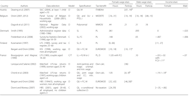
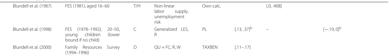
Table 1Labor supply elasticities in Europe: couples
Female wage elast. Male wage elast. Income elast. Country Authors Data selection Model Specification Tax-benefit Hours Particip. Hours Particip. Female Male Austria Dearing et al. (2007) SILC (2004), at least 1 child
aged<10
D QU; M ITABENA [.07, .19]b
Belgium Orsini (2007, 2012) Panel Survey of Belgian Households (2000–2001), working age
D QU and GU + PTD; J
MODETE [.16, .31] [.10, .19] [.10, .18] [.08, .15]
Dagsvik et al. (2011) National Register Data (2002), working age
D Polynomial MIMOSI .44 .21 .31 .18
Denmark Smith (1995) Administrative register data (1980–1986)
C SL PL .061 .093 0 −.025
Frederiksen et al. (2008) Survey by Statistics Denmark (1996), age 18–59
C SL, FC PL .148 .05 −.007 −.006
Finland Kuismainen (1997) LFS (1989), survey and tax register; 25–60
C SL, R PL [0, .06] [.11, .27]
Bargain and Orsini (2006) IDS (1998), working age, men all employed
D QU + FC; M EUROMOD [.10, .18] [.10, .17]a
France Bourguignon and Magnac (1990)
LFS (1985), couples aged 18–60
C/T LL + R; M or J PL, D 1 (.05 with FC) .10 −.03 (−.02 with FC)/−.11a
−.07
Laroque and Salanie (2002) Matched LFS-tax returns (1999), women aged 25–49
D Joint particip. and wage; unempl. and min. wage
Own calc. (.96)
Choné et al. (2003) Matched LFS-tax returns (1997), working age, children aged<6
D QU, joint wage and CC; min. wage
Own calc. 1.05 [.8, .9]b −.19 /−.18a
Bargain and Orsini (2006) HBS (1994/5), working age women, men all employed
D QU + FC; M EUROMOD [.52, .65] [.46,.58]a
Donni and Moreau (2007) HBS (2001), aged 20–60, all employed, no children aged<3
C QL; s-conditional collective LS
IZA
Journal
of
Labor
Economics
(2016) 5:10
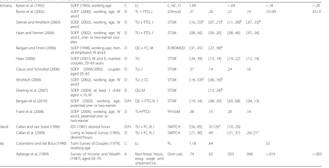
Table 1Labor supply elasticities in Europe: couples(Continued)
Germany Kaiser et al. (1992) SOEP (1983), working age C LL C, NC, D 1.04 −.04 −.18 −.28
Bonin et al. (2002) SOEP (2000), working age, W and E
D TL + PTD; J IZAmod .27 .20 .21 .19 .15/.09 .01/ 0
Steiner and Wrohlich (2004) SOEP (2002), working age, W and E
D TU + PTD; J STSM [.16, .55]b [.07, .21]b [.11, .38]b [.07, .23]b
Haan and Steiner (2004) SOEP (2002), working age, W and E, one- or two-earner cou-ples
D TU + PTD; J STSM [.08, .56] [.04, .20] [.08, .46] [.07, .26]
Bargain and Orsini (2006) SOEP (1998), working age, men all employed, W and E
D QU + FC; M EUROMOD [.31, .45] [.27, .38]a
Haan (2006) SOEP (2001), W and E; married couples, 20–65 years
D TU STSM [.34, .39] [.13, .14] [.19, .22] [.12, .14]
Clauss and Schnabel (2006) SOEP (2004/2005), couples aged 20–65
D TU; J STSM .37 .14 .24 .16
Wrohlich (2006) SOEP (2002), working age, W and E
D TU; J; CC STSM [.14, .53]b [.06, .16]b
Dearing et al. (2007) SOEP (2004), at least 1 child aged<10, W
D QU; M STSM [.13, .24]b
Bargain et al. (2010) SOEP (2003), working age, potential one- or two-earner
D/H QU + PTD, R; J STSM [.19, .34] [.08, .20] [.05, .08] [.04, .13]
Fuest et al. (2008) SOEP (2004), working age, W and E, potential one- or two-earner
D TU+PTD;J FiFoSiM .38 .15 .20 .14
Ireland Callan and van Soest (1996) IDS (1987), desired hours D/H TU + FC, R; J SWITCH [.50, .85] .31/.20a [.10, .20] Callan et al. (2009) Living in Ireland Survey (1995),
desired hours
D TU + FC, R; J SWITCH [.71, .90] .49 [.21, .31] .20/.21a
Italy Colombino and del Boca (1990) Turin Survey of Couples (1979), working age
C LL PL 1.18 .64 .52
Aaberge et al. (1999) Survey of Income and Wealth (1987), aged 20–70
A Non-linear hours, exog. wage and unearned inc.
IZA Journal of Labor Economics (2016) 5:10
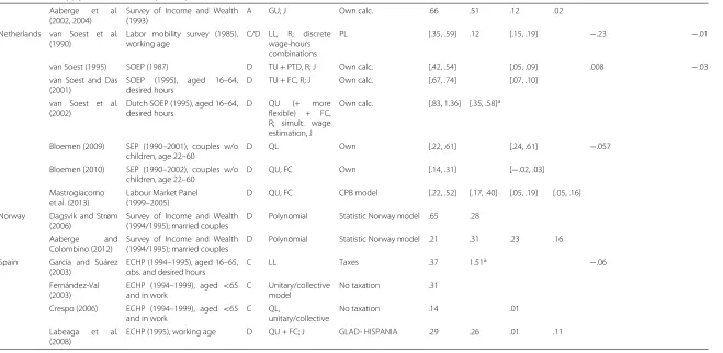
Table 1Labor supply elasticities in Europe: couples(Continued)
Aaberge et al. (2002, 2004)
Survey of Income and Wealth (1993)
A GU; J Own calc. .66 .51 .12 .02
Netherlands van Soest et al. (1990)
Labor mobility survey (1985), working age
C/D LL, R; discrete wage-hours combinations
PL [.35, .59] .12 [.15, .19] −.23 −.01
van Soest (1995) SOEP (1987) D TU + PTD, R; J Own calc. [.42, .54] [.05, .09] .008 −.03 van Soest and Das
(2001)
SOEP (1995), aged 16–64, desired hours
D TU + FC, R; J Own calc. [.67, .74] [.07, .10]
van Soest et al. (2002)
Dutch SOEP (1995), aged 16–64, desired hours
D QU (+ more flexible) + FC, R; simult. wage estimation, J
Own calc. [.83, 1.36] [.35, .58]a
Bloemen (2009) SEP (1990–2001), couples w/o children, age 22–60
D QL Own [.22, .61] [.24, .61] −.057
Bloemen (2010) SEP (1990–2002), couples w/o children, age 22–60
D QU, FC Own [.14, .31] [−.02, .03]
Mastrogiacomo et al. (2013)
Labour Market Panel (1999–2005)
D QU, FC CPB model [.22, .52] [.17, .40] [.05, .19] [.05, .16]
Norway Dagsvik and Strøm (2006)
Survey of Income and Wealth (1994/1995); married couples
D Polynomial Statistic Norway model .65 .28
Aaberge and Colombino (2012)
Survey of Income and Wealth (1994/1995); married couples
D Polynomial Statistic Norway model .21 .31 .23 .16
Spain García and Suárez (2003)
ECHP (1994–1995), aged 16–65, obs. and desired hours
C LL Taxes .37 1.51a −.06
Fernández-Val (2003)
ECHP (1994–1999), aged <65 and in work
C Unitary/collective model
No taxation .31
Crespo (2006) ECHP (1994–1999), aged <65 and in work
C QL,
unitary/collective
No taxation .14 .01
Labeaga et al. (2008)
IZA Journal of Labor Economics (2016) 5:10
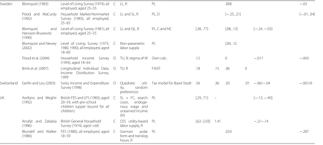
Table 1Labor supply elasticities in Europe: couplesContinued
Sweden Blomquist (1983) Level of Living Survey (1974), all employed, aged 25–55
C LL, R PL .008 −.03
Flood and MaCurdy (1992)
Household Market-Nonmarket Survey (1983), all employed, 25–65
C LL and SL, R PL, D [−.25, .21] [−.01, .04]
Blomquist and Hansson-Brusewitz (1990)
Level of Living Survey (1981), all employed, aged 25–55
C LL and QL, R PL, C and NC [.38, .77] [.08, .13] [−.24,−.03]
Blomquist and Newey (2002)
Level of Living Survey (1973, 1980, 1990), all employed, aged 18–60
C Non-parametric labor supply
PL [.04, .12
Flood et al. (2004) Household Income Survey (1993), aged 18–64
D TU, R; stigma of W Own calc. .12 0 −.017 −.003
Brink et al. (2007) Longitudinal Individual Data, Income Distribution Survey, 1999
D TU, R FASIT .18 .15 .06 0
Switzerland Gerfin and Leu (2003) Swiss Income and Expenditure Survey (1998)
D Quadratic util-ity, random preferences
Tax model for Basel-Stadt .56 .36 .03 .01 −.06/−.04 −.001/0
UK Arellano and Meghir (1992)
British FES and LFS (1983), aged 20–59, with pre-school children (upper bound for all children)
C SL + FC, search costs, endoge-nous wage and unearned income (IV)
PL [.29, .71] – [−.13,−.40]
Arrufat and Zabalza (1986)
British General Household Survey (1974), aged<60
C CES utility-based labor supply, R
PL [.62–2.03] 1.41 −.2/−.14
Blundell and Walker (1986)
FES (1980), all employed, aged 18–59
C Gorman polar form and translog hours, R
IZA
Journal
of
Labor
Economics
(2016) 5:10
Table 1Labor supply elasticities in Europe: couples(Continued)
Blundell et al. (1987) FES (1981), aged 16–60 T/H Non-linear labor supply, unemployment risk
Own calc. [.0, .408]
Blundell et al. (1998) FES (1978–1992), 20–50, young children (lower bound if no child)
C Generalized LES, R
PL [.13, .37]b – [−.19, 0]b
Blundell et al. (2000) Family Resources Survey (1994–1996)
D QU + FC, R, W TAXBEN [.11–.17]
Data: Income Distribution Survey (IDS), Household Budget Survey (HBS), Socio-Economic Panel (SOEP), Family Expenditure Survey (FES), Labor Force Survey (LFS), EU Statistics on Income and Living Conditions (SILC). For Germany: West (W), East (E). Model: C = continuous labor supply (Hausman 1981 type); T = tobit model; D = discrete-choice model (van Soest 1995 type); A = estimation of joint distributions of wage and hours (sets of hour-wage opportunities vary across individuals); H = double hurdle model (labor supply and risk of unemployment). Specification: for Hausman model, labor supply is either linear (LL), quadratic (QL), or semi-log (SL); in discrete-choice models, utility is either quadratic (QU), translog (TU), or generalized Stone-Geary (GU); random preferences are sometimes accounted for (R) as well additional flexibility, either through fixed costs (FC) or part-time dummies (PTD). Models are
male-chauvinistic (M) or account for joint decision in couples (J). Welfare program participation (W). Childcare costs (CC). Tax-benefit: Hausman model often accounts for piecewise linear budget set (PL) or more generally convex set (C); non-convexities are sometimes accounted for (NC); differentiability of the budget function can be used (D); with discrete choice models, complete tax-benefit systems are simulated and we indicate the name of the
IZA
Journal
of
Labor
Economics
(2016) 5:10
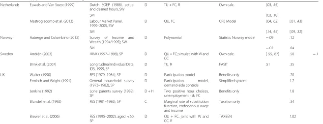
Table 2Labor supply elasticities in Europe: single individuals
Wage elast. Income
Country Authors Data selection Model Specification Tax-benefit Hours Particip. Elast.
Belgium Dagsvik et al. (2011) National Register Data, 2002, working age, SW
D Polynomial MIMOSI .13 .07
SM .2 .11
Finland Bargain and Orsini (2006) IDS (1998), SW, SP D QU + FC EUROMOD [.18, .34] [.18, .33] France Bargain and Orsini (2006) HBS (1994/1995), aged 25–49,
SW, SP
D QU + FC EUROMOD [.08, .14] [.04, .07]
Laroque and Salanie (2002) LFS-tax return matched dataset (1999), women aged 25–49, no civil servants, SW
D Participation (and full/part-time) model, simultaneous wage and labor supply estimation, probability of unemployment, min. wage
Own calc. .36
Germany Bargain and Orsini (2006) SOEP (1998), SW, SP D QU + FC EUROMOD [.09, .18] [.08, .15] Steiner and Wrohlich (2004) SOEP (2003), SW D TU + PTD STSM [.20, .36] [.05, .09]
Haan and Steiner (2004) SOEP (2002), SW D TU + PTD STSM [.02, .24] [.01, .10]
SM [.08, .31] [.04, .28]
Clauss and Schnabel (2006) SOEP (2004/2005), aged 20–65, SW
D TU + PTD STSM .38 .18
SM .23 .17
Haan and Uhlendorff (2007) SOEP (2000-2005), age 25–59, SM
D Reduced form risk model; non-parametric random coefficient
STSM [.016, .036] [.05, .12]
Fuest et al. (2008) SOEP (2004), working age, SW D TU + PTD FiFoSiM .28 .13
SM .28 .17
Bargain et al. (2010) SOEP (2003), working age, SW D/H QU + PTD; involuntary unemployment
STSM [.06, .16] [.04, .10]
SM [.10, .20] [.05, .12]
Italy Aaberge et al. (2002) Survey on Household Income and Wealth (1993), SW
A GU Own calc. .10 .06
IZA
Journal
of
Labor
Economics
(2016) 5:10
Table 2Labor supply elasticities in Europe: single individuals(Continued)
Netherlands Euwals and Van Soest (1999) Dutch SOEP (1988), actual and desired hours, SW
D TU + FC, R Own calc. [.03, .45]
SM [.03, .18]
Mastrogiacomo et al. (2013) Labour Market Panel, 1999–2005, SW
D QU, FC CPB Model [.04, .62] [.01, .43]
SM [.14, .45] [.09, .32]
Norway Aaberge and Colombino (2012) Survey of Income and Wealth (1994/1995); SW
D Polynomial Statistic Norway model −.09 .12
SM −.02 .04
Sweden Andrén (2003) HINK (1997–1998), SP D QU + FC; simulat. with W and CC
Own calc. [ .55, .87] .50 −.1
Brink et al. (2007) Longitudinal Individual Data, IDS, 1999, SP
D TU, R FASIT .51 .35
UK Walker (1990) FES (1979–1984), SP D Participation model Benefits only .70
Ermisch and Wright (1991) General household survey (1973–1982), SP
D Participation model, demand-side controls
Simplified system 1.7
Jenkins (1992) Lone parents survey (1989), SP
D + H Two positive hour choices, unemployment risk, FC
Benefits only 1.8
Blundell et al. (1992) FES (1981–1986), SP C Marginal rate of substitution function, endogenous wage and income
Taxation only .34
Brewer et al. (2006) FES (1995–2002), aged<60, SP
D QU + FC, joint with W and CC, R
TAXBEN 1.02
IZA
Journal
of
Labor
Economics
(2016) 5:10
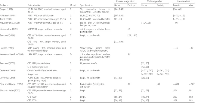
Table 3Labor supply elasticities for the USA
Female wage elast. Male wage elast. Income elast.
Authors Data selection Model Specification Hours Particip. Hours Particip. Female Male
Cogan (1981) US NLSW 1967, married women aged 30–35
C SL; reservation hours to account for FC; no tax-benefit
[.86 , 2.40] [.16 , .66]
Hausman (1981) PSID 1975, married women C LL, PL (C and NC: FC) [.90 , 1.00] [−.13,−.12] Triest (1990) PSID 1983, married women, aged 25–55 C LL; C and PL; taxes and benefits [.03 , .28] [−.15,−.19] MaCurdy et al. (1990) PSID 1975: married men, aged 25–55 C LL; PL and D (reconvexified)
budget set; taxes
[−.24, .03] −.01
Dickert et al. (1995) SIPP 1990, single mothers, no assets D Joint program and labor force participation
.35
Pencavel (1998) CPS 1975–1994, married women, aged 25–60
C Log-L; no tax-benefit [.77, .1.80]
CPS 1975–1994, single women, aged 25–60
[.77, .1.80]
Hoynes (1996) SIPP panel, 1984, married men and women with children
D Stone-Geary; stigma from
AFDC; tax-benefit system; FC −
.46 −.12
Keane and Moffitt (1998) 1994 SIPP, single mothers, no assets D Joint labor supply and welfare program participation; benefits but no tax
.96
Pencavel (2002) CPS 1999, married men C LL; no tax-benefit [.12, .25]
CPS 1999, single men [.12, .25]
Devereux (2003) Census and PSID, married men C Log-L, no tax-benefit [−.022, .017] [−.061, .001]
Single men [−.022, .017] [−.061, .001]
Devereux (2004) PUMS 1980, 1990, married couples (participating men)
C Log-L, no tax-benefit [.17, .38] [.00, .07]
Eissa and Hoynes (2004) CPS 1985 to 1997, less educated married couples with children
D Participation Probit, joint estimation
.27 .03 −.039 −.007
Blau and Kahn (2007) CPS 1980, married men and women age 25–54
C Log-L [.77, .88] [.01, .07] .004 .001
CPS 1990 C Log-L [.58, .64] [.10, .14] .002 .002
IZA
Journal
of
Labor
Economics
(2016) 5:10
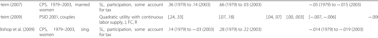
Table 3Labor supply elasticities for the USA(Continued)
Heim (2007) CPS, 1979–2003, married women
SL, participation, some account for tax
.36 (1979) to .14 (2003) .66 (1979) to .03 (2003) −.05 (1979) to−.015 (2003)
Heim (2009) PSID 2001, couples Quadratic utility with continuous labor supply, J, FC, R
[.24, .33] [.07, .18] [.04, .07] [.00, .003] [−.007,−.006] −.0007
Bishop et al. (2009) CPS, 1979–2003, sing. women
SL, participation, some account for tax
.14 (1979) to−.03 (2003) .28 (1979) to .22 (2003) −.014 (1979) to−.019 (2003)
tion, and most estimates stand in a narrow range between 0 and .30. These conclusions do not change radically if we consider more specific types of elasticities, namely total hour elasticities or participation elasticities (detailed results available from the authors). We now discuss each demographic group specifically.
3.2 Demographic groups
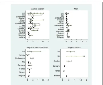
Married women Considering Tables 1 and 3, we observe much dispersion in estimates for married women. This is confirmed in Fig. 2 (top-left quadrant) where we plot the distribution of wage-elasticity estimates for each country. The black triangular cursors indicate mean values over all available estimates for each country. Mean elasticities for the UK and the USA hide a very broad dispersion across studies. Difference in elasticity size may be driven by heterogeneity in work preferences across countries and over time or by methodological reasons.
As far as genuine international differences are concerned, we suggest that larger wage elasticities prevail in countries where women’s participation is low: This seems to be the case in our survey estimates for Ireland and Italy, which is confirmed in the discussions in Callan et al. (2009) and Aaberge et al. (2002) for these two countries, respectively. In con-trast, women’s participation is high in Nordic countries and participation elasticities tend to be fairly small there, notably in Finland and Denmark and also Sweden and Norway. An exception is Blomquist and Hansson-Brusewitz (1990) for Sweden, but the authors examine data from the 1980s. Comparing Italy and Norway/Sweden, Aaberge et al. (1999) show that lower participation rates among married women in Italy leads to a larger poten-tial for reforms that increase financial incentives to work. Larger elasticities coincide with more intermittent labor force participation patterns in Southern countries and Ireland, as opposed to more consistent participation and more constant hours in Scandinavian countries. Apart from these extreme cases, differences across EU countries, and notably countries of Continental Europe, may not be very large, as suggested by Evers et al. (2008). This is confirmed by Bargain et al. (2014): Using a harmonized framework for 17 EU countries and the USA, for the same time period, they find estimates for married women ranging in a narrow interval .2–.6. This is indeed where mean values lie in Fig. 2 (top-left quadrant), with few exceptions. They also confirm that most of the responses occur at the extensive (participation) margin. Contrary to this study, our meta-analysis addresses comparisons across studies based on different methodological options, notably the period of investigation and the estimation method. We investigate the role of these two factors in the next subsection.
USA (Dickert et al. 1995) while other papers point to much larger elasticities (e.g., Keane and Moffitt 1998, for the USA or many of the British studies). The largest responses occur at the extensive margin in the UK, with very high participation elasticities on data from the 1990s and also in more recent studies (Brewer et al. 2006).
It is noticeable that the group of single parents has become much larger in the recent period. This is particularly the case in Anglo-Saxon countries, which implies possible changes in the selection effect. That is, this group may be less negatively selected in terms of labor market participation in the recent period. For the USA, Bishop et al. (2009) study all single women over a long period (1979–2003), using a simple estimation of hours and participation on repeated cross sections. They report a significant decline in hour-wage elasticities over the period and relatively small elasticities in the recent years (at least compared to typical estimates for married women).
Men and childless single individuals There is a long history of estimating male labor supply (see surveys of Hausman 1985b and Pencavel 1986, for married men). Estimates of wage elasticities for this group are usually very small, often not significant, and sometimes negative. Studies reported in Table 1 broadly confirm these stylized facts for married men. There are few exceptions, with larger elasticities in Ireland and in some of the German studies. Evidence for childless single men and women, gathered in Table 2, is relatively limited, despite the growing proportion of this demographic group in the population.
This limited evidence is essentially explained by methodological reasons. First, esti-mates are usually more precise for couples or single mothers than for childless single individuals. This can be due to the fact that there is less variation in labor market behavior among childless singles or that non-participation corresponds more often to demand-side constraints (rather than to voluntary choice) in their case. This argument equally applies to single men—yet the fit of labor supply model for married men should be overall bet-ter when male and female decisions are jointly estimated. Second, estimates stemming from natural experiments are also limited for this group, given the fact that most wel-fare reforms in Anglo-Saxon countries concerned individuals or households with children (see the discussion in Bargain and Doorley 2011). The few available estimates point to very small elasticities.13 For both men (married or single) and childless single women, estimates are not only small but also very similar between studies for each country. This small variance across studies is illustrated in Fig. 2 (top-right quadrant for men and bottom-left quadrant for childless single women). Nonetheless, these mean values may hide much variation in participation responses across different wage or income groups, with important implications for welfare analysis as suggested by Eissa and Liebman (1996) and confirmed for single individuals in Bargain et al. (2014).
3.3 Income elasticities
Bargain et al. (2014) and neither in Tables 1, 2, and 3 here. Note that very few estimates of income effects are available for single individuals.Since income effects tend to be small, in most cases, compensated and uncompensated wage elasticities are almost identical and very few studies report both. While Bargain et al. (2014) report both types of elasticities, they do not find big differences, in line with their small income elasticities.
4 Meta-analysis of the relative contributions of time changes and estimation methods
In Tables 1, 2, and 3 and Figs. 1 and 2, we have observed much variationacross studiesin the size of wage elasticities, especially for married women and single mothers. Studies that rule out differences in estimation methods and data years show that little of this is due to genuine variation in preferencesacross countries(Bargain et al. 2014). We investigate here the relative roles of time variation and estimation methods in explaining the diversity of elasticity estimates.
4.1 Graphical analysis
We begin our investigation of the respective contributions of time change versus esti-mation methods by relying on simple visual inspections. We focus our meta-analysis on married women and single mothers.
both married women and single mothers. Given the small number of US studies report-ing estimates for the latter group, we focus on married women in the right quadrant of Fig. 3 where we distinguish between EU and US estimates. The trend is similar in both regions, with a strong negative correlation between the period of observation and the elas-ticity level.14These findings tend to corroborate the result of Heim (2007) and Blau and Kahn (2007), who show that the labor supply elasticity of married women has strongly declined over time in the USA. They suggest a change in work preferences of women as possible explanation, but other explanations are possible (change in childcare policies, in domestic technology, etc.). Our results reveal that a similar trend exist for EU countries. Yet, estimates in Heim (2007) and Blau and Kahn (2007) rely on a uniform approach for the different periods while our meta-analysis possibly mixes time effects and changes in modeling and estimation methods over time.
Estimation methods To investigate this point further, let us go back to survey Tables 1, 2, and 3. A first observation is that early evidence using the Hausman technique points to relatively large own-wage elasticities for married women, sometimes close to 1, or even larger, for instance, in early studies for France, Germany, Italy, or the UK. In contrast, recent evidence based on discrete-choice models shows more modest elasticities for this demographic group, in a range between .1 and .5, with some exceptions. In Table 3, we observe a similar pattern for the USA, with very large estimates in early studies, including Hausman (1981), and more modest and comparable elasticities in the recent studies (total hour-wage elasticities ranging between .2 and .4, for instance, in Eissa and Hoynes 2004 or Heim 2007, 2009). Hence, we can conjecture that the estimation method explains time differences.
truly decline over time or whether this pattern is due to changes in estimation methods, we compare the trends in elasticities obtained with the two main methods.15 That is, Fig. 4 plots against data years the estimates obtained with continuous models (which rely mainly on the Hausman approach) and those from discrete-choice models (as recently used in many policy papers). Graphs in the upper panels show that the former was mainly used before 1990 while the latter approach took over in the 1990s and 2000s.
For continuous models, there are nonetheless some observations in the more recent years so that we can suggest tentative interpretations. For our group of interest, and whether single mothers are included (upper panel, right) or not (left), the time shrinking elasticity hypothesis is verified over all estimates relying on the Hausman approach. The linear correlation between time and elasticity size is around−.55 for married women with or without single mothers. When differentiating between regions and focusing on mar-ried women, in the lower panels of Fig. 4, this meta-analysis corroborates the findings in Heim (2007) and Blau and Kahn (2007) for the USA (both studies relying on a Hausman-type approach) and also finds a similar pattern for EU countries. Yet, it is noticeable that there are very few estimates based on the Hausman model for the period after 1990 in the EU, so the result is more fragile than for the USA.
correlation between years and estimates due to the high density of very low estimates in the years 2000s. Over all years, this correlation is−.37 for married women (going down to−.22 if German estimates, which are numerous in this period, are taken out) and−.47 when adding single mothers (−.40 without Germany). If we take out the 2000s, it goes down to−.08 for married women and−.34 when adding single mothers (Germany does not change the picture this time). For a comparison, the correlation between years and Hausman estimates remain at−.47 over this subperiod (with or without single moth-ers). The lower panel confirms results for the EU while too few estimates based on discrete-choice models exist for the USA to attempt any interpretation.
4.2 Meta-regression analysis
To disentangle time changes and estimation methods, we finally proceed with simple meta-estimations.16 Focusing first on married women, we regress elasticity values for a set of simple model characteristics.17Results are reported in Table 4. Reflecting our dis-cussion above on the limits of our observations, the first columns focus on data years for which we can find some common support in the use of the two empirical methods. That is, we restrict our sample to a period starting with the data year of the first estimate obtained with a discrete-choice model (estimates on CPS 1985 in Eissa and Hoynes 2004 and on the Dutch Labor Mobility Survey 1985 in van Soest et al. 1990). The main conclu-sion is that estimation periods (“year”) turn out to play a significant role. An additional year decreases wage elasticities of married women by around .013, which amounts to a decrease of .31 over a period of 24 years (the duration considered in Heim 2007). This conclusion holds whether we include the estimation method (a “discrete model” dummy) or not. In contrast, the estimation method is itself broadly insignificant. That is, the “over-estimation” due to the Hausman model is not particularly visible when time effects are taken into account.
IZA
Journal
of
Labor
Economics
(2016) 5:10
Table 4Meta-regression of married women’s wage elasticities
On years with common support for the use of both Hausman and discrete modelsa On all yearsb Model All elasticities Participation elasticities Hourelasticities Without the US All elasticities
Year −0.013*** −0.013*** −0.012** −0.012* −0.013** −0.024*** −0.024***
(.005) (.005) (.007) (.006) (.005) (.004) (.004)
Discrete model 0.012 0.013 0.170 −0.007 0.043 −0.236** −0.012
(.083) (.079) (.251) (.098) (.090) (.095) (.089)
Desired hours 0.258*** 0.185** 0.185** 0.086 0.837** 0.177** 0.253** 0.120 0.121
(.077) (.078) (.079) (.114) (.106) (.083) (.109) (.094) (.095)
Joint decision −0.068 −0.022 −0.026 −0.087 0.024 −0.013 −0.043 0.005 0.008
(.063) (.057) (.062) (.085) (.088) (.067) (.083) (.066) (.071)
Fixed costc 0.007 0.027 0.025 −0.024 0.069 0.014 0.007 0.039 0.041
(.059) (.055) (.057) (.074) (.082) (.060) (.082) (.067) (.070)
US −0.050 −0.049 −0.045 −0.083 0.006 −0.015 −0.044 −0.046
(.088) (.081) (.084) (.150) (.108) (.098) (.080) (.083)
Constant 0.341*** 0.470*** 0.462*** 0.323 0.454*** 0.439*** 0.569*** 1.025*** 1.025***
(.068) (.062) (.079) (.283) (.089) (.085) (.069) (.096) (.096)
Nb of observations 75 75 75 32 43 67 90 90 90
R2 0.16 0.24 0.24 0.27 0.30 0.22 0.15 0.40 0.40
Note: we regress elasticity values on modeling choices using estimates onadata from 1985 to 2004 andbdata from 1967 to 2004 cWork cost specification in discrete models
observed hours, which inflates hour-wage elasticities. This necessarily reflects the role of demand-side or institutional constraints on working time and the fact that models esti-mated on observed work duration do underestimate potential labor supply responses. Finally, Table 5 reports meta-estimates for a larger group including married women and single mothers. Results are qualitatively very similar to those for married women alone. The only visible difference is the slightly large time effect obtained for participa-tion elasticities compared to hour elasticities. This echoes our discussion in the survey (Section 3.2) about the importance of the extensive margin for the group of single mothers, especially in the UK.
5 Conclusions
In this paper, we provide an extensive survey of studies estimating static labor supply elasticities for Western Europe and the USA. We do not only confirm most of the usual stylized facts from older reviews but also derive original results concerning the variation in labor supply responses across studies. While Bargain et al. (2014) show that interna-tional heterogeneity in work preference matters but is small, we investigate the role of two factors that greatly influence the variance in elasticity size across studies, namely the time period and the estimation method. It is often suspected that large elasticities found in the literature are due to either labor market conditions of the 1970s and 1980s (and notably more intermittent female labor market participation than in the recent period) and/or to the use of a Hausman-type of model estimation (which tend to overestimate responses in some of its specifications). More recent estimates based on structural discrete-choice models with tax-benefit simulations show smaller estimates and relatively more similarity across studies. Our meta-analysis confirms that elasticities for married women and single mothers have indeed declined over time in the USA (as shown in Heim 2007 and Blau and Kahn 2007) and also in the EU. This time effect reflects a possible change in work pref-erences (and a stronger attachment of women to the labor market), in social prefpref-erences (embodied in public childcare policies), and in domestic technologies. In contrast, we find less compelling evidence that the choice of estimation method explains much variation in estimates.
Further validation of these results can be obtained at the price of an extensive estima-tion of discrete-choice models over the long period. This would also facilitate tests of the explanations underlying the shrinking elasticity hypothesis of Heim (2007) and Blau and Kahn (2007). In particular, a change in preferences over the past four decades can be tested directly on the preference parameters revealed by discrete-choice model esti-mations. This would require data since at least the early 1980s (and if possible since the 1970s) and tax-benefit simulations for all the years since these periods, in order to use policy change for robust identification. This research avenue is tedious but clearly feasible for some countries for which comparable data are available over the long run (the USA, the UK, and Germany in particular).
IZA
Journal
of
Labor
Economics
(2016) 5:10
Table 5Meta-regression of married women and single mothers’ wage elasticities
On years with common support for the use of both Hausman and discrete modelsa On all yearsb Model All elasticities Participation elasticities Hourelasticities Without the US All elasticities
Year −0.020*** −0.020*** −0.033*** −0.011* −0.018*** −0.025*** −0.028***
(.006) (.006) (.010) (.006) (.006) (.004) (.004)
Discrete model 0.004 0.042 −0.230 0.019 0.121 −0.148* 0.122
(.097) (.092) (.279) (.083) (.108) (.090) (.088)
Desired hours 0.225** 0.131 0.127 −0.093 0.246** 0.133 0.215* 0.104 0.083
(.103) (.100) (.101) (.184) (.101) (.099) (.126) (.109) (.109)
Fixed costc −0.065 −0.015 −0.022 −0.113 0.053 −0.041 −0.105 −0.003 −0.024
(.071) (.066) (.068) (.111) (.074) (.067) (.086) (.073) (.074)
US 0.052 0.024 0.035 −0.099 −0.001 0.027 −0.028 −0.001
(.103) (.094) (.097) (.181) (.106) (.104) (.087) (.089)
Constant 0.372*** 0.596*** 0.565*** 1.053*** 0.444*** 0.478*** 0.566*** 1.111*** 1.106***
(.091) (.076) (.102) (.315) (.088) (.108) (.078) (.108) (.107)
Nb of observations 90 90 90 42 48 79 108 108 108
R2 0.06 0.17 0.18 0.29 0.26 016 0.08 0.33 0.34
Note: we regress elasticity values on modeling choices using estimates onadata from 1985 to 2004 andbdata from 1967 to 2004
cWork cost specification in discrete models
it should be emphasized that there is not one “right” elasticity. A labor supply elastic-ity per se is not a deep structural parameter and depends on many factors including the country (wage distribution, institutions, labor market characteristics), the demographic group under investigating, and the time period, among others. It seems that country-specific preferences are not the primary concern. From the amount of evidence collected and discussed in this paper, policy simulations should rather make use of estimates that are derived from data collected close to the time period that analysts are looking at and for the particular demographic groups affected by the policies under study. Making the “right” choice is not easy, and we suggest using a range of “plausible” values for sensi-tivity checks. One may want to avoid using reduced-form estimates which lack external validity, if simulations imply important changes in a wide range of policies. As for estima-tions of new elasticities (our survey has shown that there are very few estimates available for some countries and some periods), one may prefer discrete-choice models than other structural approaches like the Hausman model. We found not clear evidence for sig-nificant average differences in elasticity sizes, and the critiques of the Hausman model might be overstated. However, as discussed in Section 2, discrete models usually provide a more comprehensive setting that accounts for the complete set of fiscal and social incen-tives, for explicit intensive versus extensive margins of response, and for joint decisions within couples. Estimates in our survey also show less variability across studies, conveying that the Hausman approach is too sensitive to specification choices. Whatever the struc-tural approach used for policy simulations, however, better identification strategies may be required than tax non-linearities in cross-sectional data. Identification of behavioral parameters may rely on exogenous variation from tax reforms (as in Blundell et al. 1998), experimental data, or quasi-experiments like discontinuities (Bargain and Doorley 2016).
Endnotes
1Bargain et al. (2014) conduct an estimate labor supply elasticities for 17 European
countries and the USA, separately by gender and marital status. Measurement differ-ences are netted out by using a harmonized empirical approach and comparable data sources and years. Bargain et al. (2014) find that own-wage elasticities are relatively small and much more uniform across countries than previously thought. Differences exist nonetheless and are found not to arise from different tax-benefit systems or demographic compositions across countries.
2See Chetty (2012) for an interesting discussion about the potential bias in the
estima-tion of labor supply in the presence of optimizaestima-tion fricestima-tions. To cope with this problem, Chetty provides bounds on the structural elasticities derived from reduced-form esti-mates that might suffer from optimization friction bias. The derived bounds imply that frictions affect intensive margin elasticities much more than extensive margin elasticities.
3Arguably, these other margins partly relate to responses not directly pertaining to
the number of people who do not work (see Alesina et al. 2005), and factors related to the timing and the nature of labor supply adjustments in the presence of frictions (Chetty et al. 2011).
5Another approach is the reconvexification of the budget set. For instance, to
esti-mate the labor supply of married women on 1985 French data, Bourguignon and Magnac (1990) use the Hausman technique and eliminate minor non-convexities by replacing the budget set by its convex envelope. This approach is not possible for later years as the implementation of a minimum income scheme in 1988 has introduced high non-convexity in the budget constraint. Similar non-convexities arise in all countries with substantial means-tested transfers.
6See Eklöf and Sacklén (2000) for a critical discussion of the MaCurdy critique.
7This issue is shared with the literature on the elasticity of taxable income, whereby
results are sensitive to the type of reforms exploited for identification (Saez et al. 2012). Indeed, control group definition follows from their income level, so that specific pref-erences are identified and results cannot be extrapolated. For instance, changes in tax rates (tax credits) identify the preferences of high (low)-income groups and may not be generalized to the whole population.
8Things are changing in the recent period. For France, for instance, some studies
have recently used tax-benefit changes to evaluate the responsiveness of the labor force, including the introduction of a small tax credit (Stancanelli 2008), time change in income tax schedule (Carbonnier 2008), changes in the possibility to cumulate welfare payment for lone mothers and earnings (González 2008), and age condition on children for a replacement income targeted at low-income mothers who opt for full-time childcare (Piketty 1998). RD estimations using age conditions on the level of social assistance pro-gram are also used in Bargain and Doorley (2011), in a similar way as Lemieux and Milligan (2008) for Canada.
9Note that few papers report uncompensated elasticities. One reason for this is that
income effects are often very small and, hence, compensated and uncompensated elastic-ities are almost identical. This is confirmed by the findings in Bargain et al. (2014)—one of the few studies reporting both types of elasticities.
10Note that almost all papers report elasticities with respect to the gross wage. Bargain
et al. (2014) show that net wage elasticities are—mechanically—slightly larger than gross wage elasticities.
11Note that a variety of different elasticities is used in different studies. For example,
or the income elasticity—from each paper. We have always chosen the author’s preferred estimate in case they reported several estimates (for example, as robustness checks).
13For instance, Euwals and van Soest (1999) report wage elasticities for childless single
individuals in the Netherlands of around .10–.11. For Germany, a series of studies report estimates between .10 and .36 for childless single men and women.
14We also find similar patterns when looking separately at hour-wage elasticities
(cor-relation of−.59 with observation years) and participation-wage elasticities (correlation of−.54) for married women.
15Further potentially important factors are the treatment of wages in the
estima-tion procedure (Löffler et al. 2014) and the choice of the reference tax system for the benchmark.
16Note that—like all meta-regressions—our analysis is not identifying causal effects
since one can think of several potentially omitted variables.
17Note that we cannot include all possible aspects of model specification in our paper
since there are too many dimensions and to few observations. For example, Löffler et al. (2014) investigate the role of the treatment of wages for the size of elasticities. In order to do this, the authors estimate 3500 elasticities using a discrete-choice framework with all possible permutations of model choices. Unfortunately, such a variation is missing in the estimates collected for our study.
18We do not report similar estimations for the USA only given the small number of
observations in this case.
Acknowledgements
We would like to thank Pierre Cahuc and two anonymous referees, as well as Herwig Immervoll, Max Löffler, Kristian Orsini, Sebastian Siegloch, and Carina Woodage for the useful comments on earlier drafts. The usual disclaimer applies. Responsible editor: Pierre Cahuc.
Funding
None.
Competing interests
The IZA Journal of Labor Economics is committed to the IZA Guiding Principles of Research Integrity. The authors declare that they have observed these principles.
Author details
1Aix-Marseille University (Aix-Marseille School of Economics), CNRS & EHESS, Marseille, France.2IZA, Bonn, Germany. 3ZEW, University of Mannheim, IZA and CESifo, L7, 1, 68161 Mannheim, Germany.
Received: 24 May 2016 Accepted: 7 September 2016
References
Aaberge R, Dagsvik J, Strom S (1995) Labor supply responses and welfare effects of tax reforms. Scand J Econ 97(4):635–659
Aaberge R, Colombino U, Strøm S (1999) Labour supply in Italy: an empirical analysis of joint household decisions, with taxes and quantity constraints. J Appl Econ 14:403–422
Aaberge R, Colombino U, Wennemo T (2002) Heterogeneity in the elasticity of labour supply in Italy and some policy implications, WP CHILD. #21/2002
Aaberge R, Colombino U, Strøm S (2004) Do more equal slices shrink the cake? An empirical investigation of tax-transfer reform proposals in Italy. J Popul Econ 17:767–785
Econometrica 54(1):47–63
Bargain O (2009) Flexible labour supply models. Econ Lett 105:103–105
Bargain O, Orsini K (2006) In-work policies in Europe: killing two birds with one stone Labour Econ 13:667–697 Bargain O, Caliendo M, Haan P, Orsini K (2010) Making work pay in a rationed labour market. J Popul Econ 23(1):323–351 Bargain O, Doorley K (2011) Caught in the trap? Welfare’s disincentive and the labor supply of single men. J Public Econ
95(9–10):1096–1110
Bargain, O, Doorley K (2016) Putting structure on the RD design: social transfers and youth inactivity in France. IZA Discussion Papers: 7508. Forthcoming in the Journal of Human Resources (published online before print: doi:10.3368/jhr.52.4.1115-7510R, J Human Resources July 7, 2016 1115-7510R)
Bargain O, Orsini K, Peichl A (2014) Comparing labor supply elasticities in Europe and the US: new results. J Human Resources 49(3):723–838
Bingley P, Walker I (1997) The labour supply, unemployment and participation of lone mothers in in-work transfer programmes. Econ J 107:1375–1390
Bishop K, Heim B, Mihaly K (2009) Single women’s labor supply elasticities: trends and policy implications. Ind Labor Relations Rev 63(1):146–168
Blanchard O (2006) Discussion of “Do taxes explain European employment? Indivisible labor, human capital, lotteries and savings” (by L. L.ungqvist and T. Sargent). NBER Macroeconomics Conference:2006
Blau F, Kahn L (2007) Changes in the labor supply behavior of married women: 1980–2000. J Labor Econ 25:393–438 Bloemen HG (2009) An empirical model of collective household labour supply with non-participation. Econ J 120:183–214 Bloemen HG (2010) Income taxation in an empirical collective household labour supply model with discrete hours, IZA
Discussion Papers. No:4697
Blomquist S (1983) The effect of income taxation on the labor supply of married men in Sweden. J Public Econ 22:169–197 Blomquist S, Hansson-Brusewitz U (1990) The effect of taxes on male and female labor supply in Sweden. J Hum Resour
25:317–357
Blomquist S, Newey W (2002) Nonparametric estimation with nonlinear budget sets. Econometrica 70(6):2455–2480 Blundell RW, Walker I (1986) A life cycle consistent empirical model of labour supply using cross section data. Rev Econ
Stud 53:539–558
Blundell RW, Duncan A, Meghir C (1992) Taxation and empirical labour supply models: lone parents in the UK. Econ J 102:265–278
Blundell RW, Duncan A, Meghir C (1998) Estimating labor supply responses using tax reforms. Econometrica 66:827–861 Blundell RW, Ham J, Meghir C (1987) Unemployment and female labour supply. Econ J 97:44–64
Blundell RW, MaCurdy T (1999) Labor supply: a review of alternative approaches. In: Ashenfelter and Card (eds) Handbook of labor economics, vol.3A, ch. 27. Elsevier, North-Holland
Blundell RW, Duncan A, McCrae J, Meghir C (2000) The labour market impact of the working families’ tax credit. Fiscal Studies 21(1):75–103
Blundell RW, MaCurdy T, Meghir C (2007) Labor supply models: unobserved heterogeneity, nonparticipation and dynamics, Handbook of Econometrics, Volume 6A Chapter 69 Heckman and Leamer eds
Bonin H, Kempe W, Schneider H (2002) Household labor supply effects of low-wage subsidies in Germany. J Appl Social Sci Stud 123:199–208
Bourguignon F, Magnac T (1990) Labour supply and taxation in France. J Hum Resour 25:358–389
Brewer M, Duncan A, Shephard A, Suarez MJ (2006) Did the working families’ tax credit work? The impact of in-work support on labour supply in Great Britain. Labour Econ 13(6):699–720
Brink A, Nordblom K, Wahlberg R (2007) Maximum fee versus child benefit: a welfare analysis of Swedish child-care fee reform. Int Tax Public Finance 14(4):457–480
Callan T, van Soest A (1996) Family labour supply and taxes in Ireland. ESRI working paper
Callan T, van Soest A, Walsh J (2009) Tax structure and female labour supply: evidence from Ireland. Labour 23(1):1–35 Carbonnier C (2008) Spouse labor supply: fiscal incentive and income effect, evidence from French fully joint income tax
system, working paper THEMA
Chetty R (2012) Bounds on elasticities with optimization frictions: a synthesis of micro and macro evidence on labor supply. Econometrica 80(3):969–1018
Chetty R, Guren A, Manoli D, Weber A (2011) Are micro and macro labor supply elasticities consistent? A review of evidence on the intensive and extensive margins. Am Econ Rev 101:471–75
Choné P, Le Blanc D, Robert-Bobée I (2003) Female labor supply and child care in France. CREST working paper Clauss M, Schnabel R (2006) Distributional and behavioural effects of the German labour market reform. ZEW working
paper
Cogan J (1981) Fixed cost and labour supply. Econometrica 49:945–964
Colombino U, del Boca D (1990) The effect of taxes on labor supply in Italy. J Hum Resour 25:390–414 Crespo L (2006) Estimation and testing of household labour supply models: evidence from Spain, mimeo
Dagsvik JK, Jia Z, Orsini K, van Camp G (2011) Subsidies on low-skilled workers’ social security contributions: the case of Belgium. Empir Econ 40(3):779–806
Dagsvik JK (2006) Strøm, S. Sectoral labor supply, choice restrictions and functional form. J Appl Econ 21:803–826 Dearing H, Hofer H, Lietz C, Winter-Ebmer R, Wrohlich K (2007) Why are mothers working longer hours in Austria than in
Germany? A comparative microsimulation analysis. Fisc Stud 28(4):463–495
Eissa N, Hoynes H (2004) Taxes and the labor market participation of married couples: the earned income tax credit. J Public Econ 88(9-10):1931–1958
Eissa N, Liebman J (1996) Labor supply response to the earned income tax credit. Q J Econ 111(2):605–637 Eklöf M, Sacklén H (2000) The Hausman-MaCurdy controversy: why do the results differ across studies? J Hum Resour
35(issue 1):204–220
Ermisch J, Wright R (1991) Welfare benefits and lone parents’ employment in Great Britain. J Hum Resour 26(3):424–45 Euwals R, van Soest A (1999) Desired and actual labor supply of unmarried men and women in the Netherlands. Labor
Econ 6:95–118
Evers M, de Mooij R, van Vuuren D (2008) The wage elasticity of labour supply: a synthesis of empirical estimates. De Economist 156:25–43
Fernández-Val I (2003) Household labor supply: evidence for Spain. Investigaciones Econó 27(2):239–275
Flood L, MaCurdy T (1992) Work disincentive effects of taxes: an empirical study of Swedish men. Carnegie-Rochester Conference Series on Public Policy
Flood L, Hansen J, Wahlberg R (2004) Household labour supply and welfare participation in Sweden. J Hum Ressour 39(4):1008–1032
Frederiksen A, Graversen E, Smith N (2008) Overtime work, dual job holding and taxation. Res Labor Econ 28:25–55 Fuchs VR, Krueger AB, Poterba JM (1998) Economists’ views about parameters, values, and policies: survey results in labor
and public economics. J Econ Lit 36(3):1387–1425
Fuest C, Peichl A, Schaefer T (2008) Is a flat rate reform feasible in a grown-up democracy of Western Europe? A simulation study for Germany. Int Tax Public Financ 15(5):620–636
García I SuárezMJ (2003) Female labour supply and income taxation in Spain: the importance of behavioural assumptions and unobserved heterogeneity specification. Hacienda Pública Española / Revista de Economía Pública 164(1):9–27 González L (2008) Single mothers, welfare, and incentives to work. LABOUR 22(3):447–468
Haan P, Steiner V (2004) Distributional and fiscal effects of the German tax reform 2000—a behavioral microsimulation analysis. DIW discussion paper, 419, Berlin
Haan P, Uhlendorff A (2007) Intertemporal labor supply and involuntary unemployment. IZA Discussion Paper No:2888 Hall RE (1973) Wages, income and hours of work in the U.S. labor force. In: Cain and Watts (ed). Income maintenance and
labor supply. Chicago, Markham
Hausman JA (1981) Labor supply. In: Aaron H, Pechman J (eds). How taxes affect economic behavior. The Brookings Institution, Washington DC. pp 27–72
Hausman, JA (1985a) The econometrics of nonlinear budget sets. Econometrica 53:1255–82
Hausman JA (1985b) Taxes and labor supply, Auerbach and Feldstein. In: Auerbach A, Feldstein M (eds). Handbook of public economics, vol. 1. North-Holland publishes, Amsterdam
Hausman JA, Ruud P (1984) Family labor supply with taxes. Am Econ Rev 74:242–248
Heckman JA (1993) What has been learned about labor supply in the past twenty years Am Econ Rev 83:116–121 Heim BT (2007) The incredible shrinking elasticities: married female labor supply, 1978–2002. J Hum Resour 42(4):881–918 Heim BT (2009) Structural estimation of family labor supply with taxes: estimating a continuous hours model using a
direct utility specification. J Hum Resour 44(2):350–385
Heim, BT, Meyer BD (2003) Work costs and nonconvex preferences in the estimation of labor supply models. J Public Econ 88(11):2323–38
Hotz J, Scholz K (2003) The earned income tax credit. In: Moffitt R (ed). Means-tested transfer programs in the United States. The University of Chicago Press and NBER. pp 141-197
Hoynes H (1996) Welfare transfers in two-parent families: labor supply and welfare participation under AFDC-UP. Econometrica 64:295–332
Jenkins S (1992) Lone mothers’ employment and full time work probabilities. Econ J 102(411):310–320
Kaiser H, Spahn P, van Essen U (1992) Income taxation and the supply of labour in West Germany. Jahrbü 209/1-2:87–105 Keane M, Moffitt R (1998) A structural model of multiple welfare program participation and labor supply. Int Econ Rev
39:553–589
Keane MP (2011) Labor supply and taxes: a survey. J Econ Lit 49(4):961–1075
Keane MP, Rogerson R (2012) Micro and macro labor supply elasticities: a reassessment of conventional wisdom. J Econ Lit 50(2):464–76
Killingsworth M, Heckman J (1986) Female labor supply: a survey. In: Ashenfelter O, Layard R (eds). Handbook of labor economics. North-Holland, Amsterdam Vol. 1
Kuismanen M (1997) Labour supply, unemployment and income taxation: an empirical application, Working Paper. In: Government Institute for Economic Research. University College London, Helsinki
Labeaga JM, Oliver X, Spadaro A (2008) Discrete choice models of labour supply, behavioural microsimulation and the Spanish tax reform. J Econ Inequal 6(3):247–273
Laroque G, Salanié B (2002) Labor market, institutions and employment in France. J Appl Econom 17:25–48 Lemieux T, Milligan K (2008) Incentive effects of social assistance: a regression discontinuity approach. J Econom
142(2):807–828
Löffler M, Peichl A, Siegloch S (2014) Structural labor supply models and wage exogeneity. IZA Discussion Paper No:8281 MaCurdy T (1992) Work disincentive effects of taxes: a reexamination of some evidence. Am Econ Rev Papers Proc
82:243–249
assumptions. Econometrica 55(4):765–799
Orsini K (2012) Tax benefit reforms and the labor market: evidence from Belgium and other EU countries. Labour Econ 19(1):129–138. Previously Leuven University, working paper. 2006
Orsini, K (2007) Ex-ante evaluations of tax and benefit reforms in the EU: what can we learn? Leuven University, working paper
Pencavel J (1986) Labor supply of men: a survey. In: Ashenfelter O, Layard R (eds). Handbook of labor economics. North-Holland, Amsterdam Vol. 1
Pencavel, J (1998) The market work behavior and wages of women, 1975-94. J Hum Resour 33(4):771–804 Pencavel J (2002) A cohort analysis of the association between work hours and wages among men. J Hum Resour
37(2):251–274
Piketty T (1998) L’impact des incitations financières au travail sur les comportements individuels: une estimation pour le cas français. Economie et Pré 132–133:1–35
Prescott EC (2004) Why do Americans work so much more than Europeans? Quarterly Review. Federal Reserve Bank of Minneapolis, issue Jul:2–13
Saez E, Slemrod J, Giertz SH (2012) The elasticity of taxable income with respect to marginal tax rates: a critical review. J Econ Lit 50(1):3–50
Smith N (1995) A panel study of labour supply and taxes in Denmark. Appl Econ 27(5):419–429
Stancanelli E (2008) Evaluating the impact of the French tax credit on the employment rate of women. J Public Econ 92(10–11):2036–47
Steiner V, Wrohlich K (2004) Household taxation, income splitting and labor supply incentives—a microsimulation study for Germany. CESifo Econ Stud 50(3):541–568
Triest RK (1990) The effect of income taxation on labor supply in the United States. J Hum Resour 25:491–516 van Soest A (1995) Structural models of family labor supply: a discrete choice approach. J Hum Resour 30:63–88 van Soest A, Das M (2001) Family labor supply and proposed tax reforms in the Netherlands. De Economist 149(2):191–218 van Soest A, Das M, Gong X (2002) A structural labor supply model with non-parametric preferences. J Econom (Annals)
107:345–374
van Soest A, Woittiez I, Kapteyn A (1990) Labour supply, income taxes and hours restrictions in the Netherlands. J Hum Resour 25:517–558
Walker I (1990) The effect of income support measures on the labour market behaviour of lone mothers. Fisc Stud 11(2):55–74
Wrohlich K (2006) Child care costs and mothers’ labor supply: an empirical analysis for Germany. DIW Berlin Ziliak JP, Kniesner TJ (1999) Estimating life cycle labor supply tax effects. J Polit Econ 107(2):326–59
Submit your manuscript to a
journal and benefi t from:
7 Convenient online submission 7 Rigorous peer review