Theoretical Studies of Cosmic Acceleration

(1)

University of Pennsylvania

ScholarlyCommons

Publicly Accessible Penn Dissertations

1-1-2016

Theoretical Studies of Cosmic Acceleration

James Stokes

University of Pennsylvania, jstokes2@baml.com

Follow this and additional works at:

http://repository.upenn.edu/edissertations

Part of the

Physics Commons

This paper is posted at ScholarlyCommons.http://repository.upenn.edu/edissertations/2040

Recommended Citation

(2)

Theoretical Studies of Cosmic Acceleration

Abstract

In this thesis we describe theoretical approaches to the problem of cosmic acceleration in the early and late universe. The first approach we consider relies upon the modification of Einstein gravity by the inclusion of mass terms as well as couplings to higher-derivative scalar fields possessing generalized internal shift symmetries - the Galileons. The second half of the thesis is concerned with the quantum-mechanical

consistency of a theory of the early universe known as the pseudo-conformal mechanism which, in contrast to inflation, relies not on the effects of gravity but on conformal field theory (CFT) dynamics.

It is possible to couple Dirac-Born-Infeld (DBI) scalars possessing generalized Galilean internal shift symmetries (Galileons) to nonlinear massive gravity in four dimensions, in such a manner that the interactions maintain the Galilean symmetry. Such a construction is of interest because it is not possible to couple such fields to massless General Relativity in the same way. Using tetrad techniques we show that this massive gravity-Galileon theory possesses a primary constraint necessary to ensure propagation with the correct number of degrees of freedom.

We study the background cosmology of this theory around cosmologically relevant spacetimes and find that, as in pure massive gravity, spatially flat solutions do not exist. Spatially open solutions do exist - consisting of a branch of self-accelerating solutions that are identical to those of pure massive gravity, and a new second branch of solutions which do not appear without the inclusion of Galileons. We study the propagating degrees of freedom of the massive gravity-Galileon theory around the self-accelerating solutions and identify the conditions necessary for the theory to remain free of ghost-like instabilities. We show that on the self-accelerating branch the kinetic terms for the vector and scalar modes of the massive graviton vanish, as in the case of pure massive gravity.

We conclude our exploration of massive gravity by considering the possibility of variable-mass massive gravity, where the fixed graviton mass is replaced by the expectation value of a rolling scalar field. We ask whether self-inflation can be driven by the self-accelerated branch of this theory, and we find that, while such solutions can exist for a short period, they cannot be sustained for a cosmologically useful time. Furthermore, we demonstrate that there generally exist future curvature singularities of the ``big brake" form in

cosmological solutions to these theories.

In the second half of the thesis we construct the gravitational dual of the pseudo-conformal universe, a proposed alternative to inflation in which a CFT in nearly flat space develops a time dependent vacuum expectation value. Constructing this dual amounts to finding five-dimensional domain-wall spacetimes with anti-de Sitter asymptotics, for which the wall has the symmetries of four-dimensional de Sitter space. This holographically realizes the characteristic symmetry breaking pattern O(2,4) to O(1,4) of the pseudo-conformal universe. We present an explicit example with a massless scalar field, using holographic renormalization to obtain general expressions for the renormalized scalar and stress-tensor one-point functions. We discuss the relationship between these solutions and those of four-dimensional holographic CFTs with boundaries, which break O(2,4) to O(2,3).

(3)

presented, including the holographic boundary CFTs as well as spacelike boundary CFTs, which provide realizations of the pseudo-conformal universe.

Degree Type

Dissertation

Degree Name

Doctor of Philosophy (PhD)

Graduate Group

Physics & Astronomy

First Advisor

Mark Trodden

Subject Categories

(4)

THEORETICAL STUDIES OF COSMIC ACCELERATION

James Stokes

A DISSERTATION

in

Physics and Astronomy

Presented to the Faculties of the University of Pennsylvania

in

Partial Fulfillment of the Requirements for the

Degree of Doctor of Philosophy

2016

Supervisor of Dissertation

Mark Trodden

Professor (Department of Physics and Astronomy)

Graduate Group Chairperson

Marija Drndic, Professor (Department of Physics and Astronomy)

Dissertation Committee:

Randall Kamien, Professor (Department of Physics and Astronomy)

Justin Khoury, Professor (Department of Physics and Astronomy)

Elliot Lipeles, Professor (Department of Physics and Astronomy)

(5)

c

COPYRIGHT

2016

James Stokes

This work is licensed under the

Creative Commons Attribution

NonCommercial-ShareAlike 3.0

License

(6)

Acknowledgements

First and foremost, I’d like to thank Mark Trodden his excellent supervision and for

con-stantly encouraging me to pursue my interests.

During my PhD I have had the good fortune to collaborate with and learn from many

out-standing physicists: Melinda Andrews, Garret Goon, Steven Gubser, Kurt Hinterbichler,

Austin Joyce, Justin Khoury, Burt Ovrut, Alexander Polyakov, Zain Saleem, Sam

Schoen-holz, Bogdan Stoica, and Mark Trodden. I am indebted to Randall Kamien and Tom

Lubensky for discussions on field theory and condensed matter physics.

I would like to thank all of the friends I have made during my PhD, especially my office

mates Hernan Piragua and my long-term collaborator Zain Saleem. I have always enjoyed

our discussions and debates from which I have learnt a great deal of physics.

I thank my parents and sister for their unceasing love and support, for which I am deeply

(7)

ABSTRACT

James Stokes

Mark Trodden

In this thesis we describe theoretical approaches to the problem of cosmic acceleration in

the early and late universe. The first approach we consider relies upon the modification

of Eintein gravity by the inclusion of mass terms as well as couplings to higher-derivative

scalar fields possessing generalized internal shift symmetries —the Galileons. The second

half of the thesis is concerned with the quantum-mechanical consistency of a theory of the

early universe known as the pseudo-conformal mechanism which, in contrast to inflation,

relies not on the effects of gravity but on conformal field theory (CFT) dynamics.

It is possible to couple Dirac-Born-Infeld (DBI) scalars possessing generalized Galilean

internal shift symmetries (Galileons) to nonlinear massive gravity in four dimensions, in

such a manner that the interactions maintain the Galilean symmetry. Such a construction

is of interest because it is not possible to couple such fields to massless General Relativity in

the same way. Using tetrad techniques we show that this massive gravity-Galileon theory

possesses a primary constraint necessary to ensure propagation with the correct number of

degrees of freedom.

We study the background cosmology of this theory around cosmologically relevant

space-times and find that, as in pure massive gravity, spatially flat solutions do not exist. Spatially

open solutions do exist — consisting of a branch of self-accelerating solutions that are

iden-tical to those of pure massive gravity, and a new second branch of solutions which do not

appear without the inclusion of Galileons. We study the propagating degrees of freedom

of the massive gravity-Galileon theory around the self-accelerating solutions and identify

(8)

that on the self-accelerating branch the kinetic terms for the vector and scalar modes of the

massive graviton vanish, as in the case of pure massive gravity.

We conclude our exploration of massive gravity by considering the possibility of

variable-mass variable-massive gravity, where the fixed graviton mass is replaced by the expectation value

of a rolling scalar field. We ask whether self-inflation can be driven by the self-accelerated

branch of this theory, and we find that, while such solutions can exist for a short period, they

cannot be sustained for a cosmologically useful time. Furthermore, we demonstrate that

there generally exist future curvature singularities of the “big brake” form in cosmological

solutions to these theories.

In the second half of the thesis we construct the gravitational dual of the pseudo-conformal

universe, a proposed alternative to inflation in which a CFT in nearly flat space develops a

time dependent vacuum expectation value. Constructing this dual amounts to finding

five-dimensional domain-wall spacetimes with anti-de Sitter asymptotics, for which the wall has

the symmetries of four-dimensional de Sitter space. This holographically realizes the

char-acteristic symmetry breaking pattern so(2,4)_→so(1,4) of the pseudo-conformal universe.

We present an explicit example with a massless scalar field, using holographic

renormaliza-tion to obtain general expressions for the renormalized scalar and stress-tensor one-point

functions. We discuss the relationship between these solutions and those of four-dimensional

holographic CFTs with boundaries, which break so(2,4)_→so(2,3).

Finally, we undertake a systematic study of one and two point functions of CFTs on spaces

of maximal symmetry with and without boundaries and investigate their spectral

represen-tations. Integral transforms are found, relating the spectral decomposition to renormalized

position space correlators. Several applications are presented, including the holographic

boundary CFTs as well as spacelike boundary CFTs, which provide realizations of the

(9)

List of Figures

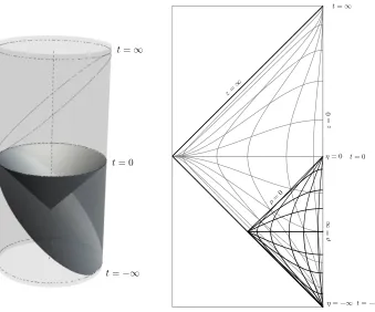
Figure 1 : Penrose diagrams showing the Poincar´e coordinates and de Sitter

slice coordinates. The left-hand figure shows the global AdS cylinder;

the de Sitter slice coordinate region is bounded from above by the

lightcone which emanates downward fromt= 0, and is bounded from

below by the slanted ellipse, which also marks the lower boundary of

the Poincare patch (the upper slanted ellipse shown in outline form

is the upper boundary of the Poincar´e patch). The right-hand figure

shows a two dimensional slice down the axis of the AdS cylinder;

thin lines are Poincar´e lines of constantzand t, thick lines de Sitter

slice lines of constantρ and η. . . 41

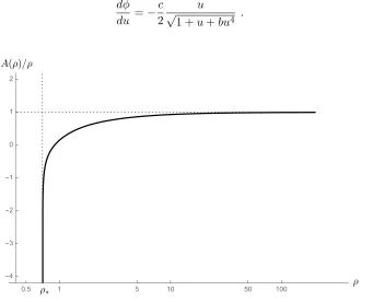
Figure 2 : A typical solution. Here b = 1. On the horizontal axis is the ρ

coordinate on a logarithmic scale, and on the vertical axis is the scale

factor A(ρ), normalized by ρ so that it can be seen that A _→ ρ as

ρ_{→ ∞}, corresponding to asymptotically AdS boundary conditions.

The singularity occurs at the value ρ∗ ≈ 0.7, for which the scale

factor goes to −∞. . . 45

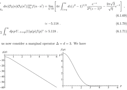
Figure 3 : Spectral representationshO2(n)O2(n0)iH3 (left) andf(~n·~n

0_{) (right)}

(13)

Chapter 1 Introduction

Modern cosmology poses a host of physics questions that demand answers from fundamental

theory. For instance: what is the resolution of the cosmic singularity? What explains the

anomalous acceleration seen in the present-day universe and what is the origin of primordial

fluctuations in the very early universe, which seeded the cosmic structure seen today? This

thesis explores possible solutions to these problems and others by drawing upon novel field

theory techniques such as infra-red modifications of gravity and dualities originating in

string theory.

One of the most perplexing puzzles in the late universe is the problem of the cosmological

constant. In classical general relativity the cosmological constant is free parameter Λ which

appears in the action for the gravitational field,

S = 1

2M

2 P

Z

d4x√−g(R[gµν]−2Λ) +Smatter[gµν,Ψ] (1.0.1)

where the first term is the Einstein-Hilbert action, the second is the cosmological constant

and the final term represents the mixing of matter fields Ψ with the gravitational fieldgµν.

Solving the Einstein field equations in a cosmogical Friedman-Roberston-Walker spacetime

we find that the cosmological constant contributes a constant term in the Friedman equation,

while all other energy components are suppressed by factors of the scale factor,

˙

a a

2

= Λ + 1

3M2 P

−k

a2 +· · ·

. (1.0.2)

where the dots represent contributions from matter fields which are suppressed by higher

(14)

the universe. The story changes signficantly when quantum mechanics is taken into account.

Vacuum fluctuations of the graviton and other fields are expected to drive the cosmological

constant to the short-distance cut-off of the theory. On the other hand, the observed cosmic

acceleration suggests that the cosmological constant is determined by the infra-red

(long-distance) cut-off. This strongly suggests that the the solution of the cosmological constant

problem lies in the infrared interactions of gravity. Recently it has become clear that a

consistent infra-red modification of gravity based on mass terms exists and can be applied

to the late universe. We will explore this theory and some of its extensions.

The late universe is not the only place where the techniques of quantum field theory can

address theoretical issues. In the very early universe we are faced with a number of

ques-tions in inflation and some of its alternatives. The prevailing hypothesis for the origin

of nearly scale-invariant temperature fluctuations observed in the cosmic microwave

back-ground is that the early universe underwent a period of exponentially accelerated expansion

called inflation (see [1] for a review) which stretched microscopic quantum fluctuations to macroscopic scales. In addition to explaining temperature anisotropies, inflation solves the

horizon problem (why the universe appears uniform across apparently causually

discon-nected regions) and the flatness problem (why the universe is spatially flat when curvature

is expected to dominate at late times). It is important to understand if these successes are

unique to inflation, and if there exist experimentally distinguishable alternatives.

Over the past decade, attempts to find a consistent infrared modification of gravity have

led to two seemingly distinct discoveries. The first is a consistent, ghost free nonlinear

realization of massive gravity, known as dRGT massive gravity [2,3]. The second is a class of intriguing scalar field theories — the Galileons [4] — with novel classical and quantum properties that can be traced to their nonlinear derivative interactions. There is at least

one connection between these ideas, in that the Galileon interactions govern the longitudinal

(15)

motion and the special symmetries of those theories, then it is natural to couple not to

General Relativity (GR) as in [5, 6] (which breaks the Galileon symmetry), but rather to massive gravity itself [7]. Thus one is led to a theory of massive gravity Galileons, which we will study extensively in this thesis.

One of the general challenges faced in modifying gravity by mass terms is to ensure that

the resulting theory propagates the correct number of degrees of freedom to describe a

massive spin-2 particle. It has long been known that the Fierz-Pauli action [8] provides a consistent description of the linear fluctuations of a massive graviton in flat spacetime.

Nonlinear theories of massive gravity, however, tend to suffer from an instability known as

the Boulware-Deser (BD) ghost [9]. The dRGT theory is a 3-parameter family of potentials whose special structure ensures that there is a dynamical constraint which removes the ghost

degree of freedom. This has been demonstrated by explicitly counting degrees of freedom

in the Hamiltonian formalism [10, 11], and through other methods [12–15]. It is therefore essential to ensure that extensions of the dRGT massive gravity theory are theoretically

well-grounded. In the first chapter we bring the techniques of field theory to bear on this

issue by proving that massive gravity coupled to Galileons propagates the correct number

of degrees of freedom. This is a crucial requirement of the theory that opens the door to

the model building in the subsequent chapters.

An appealing feature of pure dRGT massive gravity is that it admits self-accelerating

so-lutions [16–21], in which the de Sitter Hubble factor is of order the mass of the graviton. Since having a light graviton is technically natural [22,23], such a solution is of great inter-est in the late-time universe to account for cosmic acceleration. We derive the background

cosmological equations for massive gravity coupled to Galileons, and find that the presence

of the scalar leads to a more complicated constraint than in pure dRGT. We discuss the

possible solutions in the case of zero and negative spatial curvature. We find that, as in

pure dRGT theory, this constraint forbids flat FRW solutions. For an open FRW ansatz,

(16)

self-accelerating solutions that are identical to the self-accelerating solutions of pure dRGT

theory. The second branch consists of novel solutions which are not found in pure massive

gravity.

Although the dRGT theory possesses a self-accelerating solution with negatively curved

spatial slices [21], the study of fluctuations on top of this background has shown that the kinetic terms for the vector and scalar perturbations vanish [24].

It has been shown that the vanishing of these terms can be remedied by departing from

isotropic and homogeneous cosmologies [25, 26] or by introducing new degrees of free-dom. There are many ways to achieve the latter option, and several possibilities have

been explored in the so-called quasi-dilaton [27–30] and mass-varying extensions of dRGT [20,30,31]. Motivated by these examples, we perform a study of cosmological perturbations around the self-accelerating branch for the massive gravity Galileon theory and show that

the kinetic terms for the scalar and vector modes vanish, similar to the case of the pure

dRGT theory.

It is tempting to theorize that massive gravity might play a role the early universe too.

A natural question is whether massive gravity might provide an alternative to inflation by

driving accelerated expansion in the early universe. To use the self-accelerating solution

of massive gravity for inflation (i.e. “self-inflation”), the graviton mass would have to be

of order the Hubble scale during inflation. Yet, we know that the current graviton mass

cannot be much larger than the Hubble scale today [32].

Thus, for self-inflation to be possible, the graviton mass must change in time. One idea of

how to realize this is to promote the graviton mass to a scalar field, Φ, which has its own

dynamics and can roll [20, 31]. The expectation value (VEV) of Φ then sets the mass of the graviton. We can imagine that at early times Φ has a large VEV, so that the graviton

is very massive, and the universe self-inflates with a large Hubble constant. Then, at late

(17)

value consistent with present day measurements.

We will see that, in practice, such an inflation-like implementation of massive gravity is

difficult to achieve in this model. Pure dRGT theory has a constraint, stemming from

the Bianchi identity, which forbids standard FRW evolution in the flat slicing [20] (the self-accelerating solutions are found in other slicings). There appears an analogous constraint in

the variable mass theory, and this constraint, while it no longer forbids flat FRW solutions,

implies that self-inflation cannot be sustained for a cosmologically relevant length of time.

In addition, we show that non-inflationary cosmological solutions to this theory may exhibit

future curvature singularities of the “big brake” type.

In the remainder of the thesis we seek to overcome one of the challenges which is faced

by alternatives to inflation which do not rely on modified gravity. Typically such

scenar-ios involve a slowly contracting ‘pre-big bang’ phase in which the universe crunches and

subsequently expands. An interesting implementation of this idea postulates that the early

universe is described by a CFT whose conformal algebra is spontaneously broken by

oper-ator vacuum expectation values to a de Sitter subalgebra — the so-called pseudo-conformal

universe [33–36]. Despite the theoretically appealing features of this model, it is challenging to find ultra-violet-complete examples of CFTs which possess the required set of vacuum

states to realize the pseudo-conformal mechanism. In chapter 5 we address this issue by

pro-viding an explicit embedding of the pseudo-conformal mechanism in the so-called AdS/CFT

correspondence [64]. Our construction involves computing the unambiguous parts of the ex-act one-point functions of the scalar operator and stress tensor, in the presence of a general

source and boundary metric, using the techniques of holographic renormalization [106].

We will see that the holographic perspective of the pseudo-conformal universe leads us

naturally to the mathematical problem of calculating CFT correlation functions in curved

spacetimes. Such correlation functions are crucial when confronting these theories with

ob-servational cosmology. Correlation functions in general quantum field theories can present

(18)

regulariza-tion dependent and parametrize un-calculable high energy effects which are renormalized

into the undetermined local couplings of the effective action1_{. Theories without a mass}

gap exhibit long-range correlations, which can lead to infra-red singularities in Fourier

space. These are calculable universal features, not dependent on regularization ambiguities

or absorbable into local couplings. The last chapter is devoted to exploring the two-point

functions of CFTs in curved spaces such as those arising in the pseudo-conformal

uni-verse. In particular, we explain how short-distance singularities can be absorbed into local

counter-terms. The initial motivation for this work was to holographically compute

two-point functions in the pseudo-conformal universe (which would correspond to the power

spectra of interest in cosmology), but the results apply more widely to other conformal field

theories with boundaries.

1

(19)

Chapter 2 Massive Gravity Coupled to Galileons is

Ghost Free

In this chapter, we describe the explicit counting of degrees of freedom which shows that

massive gravity coupled to DBI Galileons is not afflicted by the BD ghost. Most of this

chapter is taken from [37], which was written in collaboration with Garret Goon, Kurt Hinterbichler, Mark Trodden and Melinda Andrews.

A general Lagrangian for nonlinear massive gravity can be formulated by introducing a

non-dynamical reference metric ¯gµν (e.g. the Minkowski one, ¯gµν =ηµν) and constructing a

potential of the formV(gµσ_¯_g

σν). The potential explicitly breaks diffeomorphism invariance

and it is expected that the theory generally propagates 12 phase-space degrees of freedom,

rather than the 10 necessary to describe a massive graviton. The extra degree of freedom

is the BD ghost.

The diffeomorphism invariance broken by the mass term can be restored through the

St¨uckelberg method [22], which involves introducing four auxiliary scalars φA₍_x_{) through} the replacement ¯gµν →∂µφA∂νφBηAB.The St¨uckelberg fields are pure gauge and the

orig-inal theory is recovered by choosing unitary gauge φA ₌ _δA

µxµ. In this formulation, the

scalars can be regarded as the embedding mapping of a sigma model Σ_{→ M}, where both

Σ and _Mare four dimensional Minkowski space. There is an internal Poincar´e symmetry

corresponding to the isometries of the target space. From this point of view, the dynamical

metric gµν(x) is a worldvolume metric living on Σ.

The target space may be higher dimensional, and need not be flat – we may generalize the

(20)

(so that now_A,_B,_{· · ·} run overD values) and a fixed target space metricGAB(φ),

¯

gµν =∂µφA∂νφBGAB(φ). (2.0.1)

There are now (dim_M)₋4 embedding fields which cannot be gauged away and these become

physical Dirac-Born-Infeld (DBI) scalars coupled to the physical metric through the dRGT

potential [7]. Apart from the dRGT terms, curvature invariants constructed solely from ¯gµν and extrinsic curvatures of the embedding can be included in the action. The leading term

in the derivative expansion is the DBI action ∼R

d4_x√₋_g_¯_{, and higher Lovelock invariants}

give Galileons [38,39]. The theory will possess a Galileon-like internal symmetry for every isometry ofGAB, and the resulting Galileons will be the generalized curved space Galileons

discussed in [40–43].

Apart from generalizing dRGT, the construction of [7] is of interest because it provides a method of coupling the Galileons to (massive) gravity while preserving the Galileon

invari-ance. When coupling to ordinary massless gravity, non-minimal couplings must be added

to ensure second-order equations of motion, and the Galileon symmetry is broken [5, 6]. In the present construction, there is no such problem, suggesting that the Galileons more

naturally couple to a massive graviton.

In [7], it was shown that the theory is ghost-free, for a flat target space metric, in the decoupling limit, and for a certain simplifying choice of parameters. In this chapter, using

methods similar to those of [15], we demonstrate that the full theory, for any target space metric GAB, to all orders beyond the decoupling limit, and for all choices of parameters,

(21)

2.1 The model

The dynamical variables are the physical metric gµν and the D scalars φA, which appear

through the induced metric (2.0.1). The action is

S=SEH[g] +Smix[g,g¯] +SGalileon[¯g]. (2.1.1)

HereSEH[g] is the Einstein-Hilbert action for gµν, with a possible cosmological constant Λ,

SEH[g] = M 2 P 2

Z

d4x√−g(R[g]−2Λ). (2.1.2)

The action mixing the two metrics is

Smix[g,g¯] =−

M2 Pm2

8 3

X

n=1

βnSn p

g−1_¯_g _, _(2.1.3)

wherepg−1_g_¯_{is the matrix square root of the matrix}_gµσ_¯_g

σν, andSn(M) of a matrixM are

the symmetric polynomials2 _S

n(M) = M[µµ11· · ·M

µn]

µn. The βn are three free parameters

(one combination of which is redundant with the mass m). SGalileon[¯g] stands for any

Lagrangian constructed from diffeomorphism invariants of ¯g (and extrinsic curvatures of

the embedding) whose equations of motion remain second order in time derivatives. The

possible terms inSGalileon[¯g] are the Lovelock invariants and their boundary terms (see [38] and Sec. IV.B of [39] for a discussion). The structure of the dRGT-DBI coupled system (3.0.2) is nearly identical to that of ghost-free bi-gravity [45], the difference being that one of the two metrics is induced from a target space, and so it fundamentally depends on the

embedding scalars.

Following [15], we will find it convenient to write the theory in vierbein form3_{. We write}

2_{Our anti-symmetrization weight is [}_µ

1. . . µn] = _n1_!(µ1· · ·µn+· · ·). See appendix A of [15] for more

details on the symmetric polynomials.

3_{See also [46,} _{47] for covariant methods of degree of freedom counting in the vierbein formulation of}

(22)

the physical metric and induced metric in terms of vierbeinsEA₌_E A

µ dxµ, ¯EA= ¯EµAdxµ,

gµν =EµAEνBηAB, g¯µν = ¯EµAE¯νBηAB, (2.1.4)

where ηAB is the 4 dimensional Minkowski metric. For the induced metric ¯gµν, we choose

a frame in which the vierbein is in an upper triangular form

¯

EµB = 

 

¯

N N¯i_e_¯ ia

0 e¯ia 



 . (2.1.5)

Here ¯N and ¯Ni _{are ADM lapse and shift variables, and ¯}_e

ia is an upper triangular spatial

dreibein for the spatial part of the induced metric and ¯ei

a its inverse transpose (in what

follows i, j, . . .are spatial coordinate indices raised and lowered with the spatial metric ¯gij,

and a, b, . . .are spatial Lorentz indices raised and lowered withδab). These are obtained in

terms ofφA _{by solving}

¯

g00= ˙φAφ˙BGAB(φ) =−N¯2+ ¯NiN¯i

¯

g0i = ˙φA∂iφBGAB(φ) = ¯Ni

¯

gij =∂iφA∂jφBGAB(φ) = ¯eia¯ejbδab . (2.1.6)

The upper triangular vierbein (2.1.5) has 10 components, and is merely a repackaging of

the 10 components of ¯gµν(which in turn depend on theφA).

For the physical metric gµν, we parameterize its 16 component vierbein as a local Lorentz

transformation (LLT)M, which has 6 components, times a vierbein ˆE which is constrained

in some way so that it has only 10 components,

EµA=MABEˆµB (2.1.7)

(23)

theory manifest. The mixing term (3.0.4), in terms of vierbeins, takes the form

Smix≡ −

M2 Pm2

8 3

X

n=1

βn

n!(4₋n)!S (n) mix,

S_mix(1) =

Z

ABCDE¯A∧EB∧EC ∧ED,

S_mix(2) =

Z

ABCDE¯A∧E¯B∧EC ∧ED,

S_mix(3) =

Z

ABCDE¯A∧E¯B∧E¯C ∧ED. (2.1.8)

The dynamical vierbein has 16 components, 6 more than the metric. If we choose the 6

constraints which ˆE must satisfy to be the symmetry condition,

ˆ

Eµ[AE¯µ_B_]= 0, (2.1.9)

then we can show using the arguments in [15] (see also [48] for subtleties) that the extra 6 fields in M are auxiliary fields which are eliminated by their own equations of motion,

settingM = 1, and the resulting theory is dynamically equivalent to the metric formulation

(3.0.2).

Instead, we take ˆE to be of upper triangular form

ˆ

EµA= 

 

N Ni_e ia

0 eia





. (2.1.10)

Here the spatial dreibeinea

i is arbitrary, containing 9 components. The LLT M in (2.1.7)

depends now on 3 boost parameterspa _{and can be written as}

M(p)A_B =



 

γ pb

pa δ_ba+₁₊1_γpapb 



 , (2.1.11)

where γ ≡ √1 +pa_p

(24)

pa-rameterized in terms of the 3 components of pa_{, one} _N_{, 3 components of} _Ni _{and the 9}

components of eib.

2.2 Hamiltonian analysis

We start the Hamiltonian analysis by Legendre transforming with respect to the spatial

vierbeinea

i , defining canonical momentaπia= ∂

L

∂e˙ a

i . SinceSmixcontains no time derivatives

of the physical metric, and SGalileon has no dependence on the physical metric at all, the

expressions for the canonical momenta are the same as their GR counterparts. In particular,

there will be three primary constraints

Pab=ei[aπib]= 0. (2.2.1)

In GR, these are first class constraints which generate local rotations. In our case, the local

Lorentz symmetry is broken, and these constraints will generate secondary constraints and

form second class pairs.

The Einstein-Hilbert part of the action takes the form4

SEH=

Z

d4x πi_ae˙_ia₋1 2λ

ab

Pab−NC(e, π)−NjCj(e, π). (2.2.2)

The anti-symmetric λab _{holds the three Lagrange multipliers for the three primary}

con-straints (2.2.1). TheN and Ni _{appear as Lagrange multipliers enforcing respectively the}

Hamiltonian and momentum constraints of GR: _C= 0, _Ci= 0.

We now look at the mixing terms (2.1.8). The contributions to _Lmix are of the form

∼ µνρσ

ABCDEµAEνBE¯ρCE¯σD, containing various numbers of copies of E and ¯E. From

(2.1.5), (2.1.10) and (2.1.11), we see that theµ= 0 components ofEµAand ¯EµAare strictly

linear in their respective lapses and shifts and the µ = i components are independent of

the lapse and shift. Therefore, due to the anti-symmetry of the epsilons, the entire mixing

(25)

term is linear in the lapses and shifts, so we may write

Lmix=−NCmix(e,¯e, p)−NiCmix,i(e,¯e, p)−N¯C¯mix(e,e, p¯ )

−N¯i_C¯mix,i(e,¯e, p)− Hmix(e,¯e, p) . (2.2.3)

The lapse and shift remain as Lagrange multipliers, and the pa _{appear algebraically. We}

now solve the constraint enforced by Ni _{for the} _pa_: _C

i +Cmix,i = 0 ⇒ pa = pa(e,e, π¯ ).

Plugging back into the action we obtain

S=

Z

d4x πi_ae˙_ia−1

2λ ab_P

ab−N[C(e, π) +Cmix(e,¯e, π)]

−N¯C¯mix(e,e, π¯ )−N¯iC¯mix,i(e,e, π¯ )

− Hmix(e,e, π¯ ) +LGalileon(¯e,N ,¯ N¯i) . (2.2.4)

It remains to Legendre transform with respect to the scalarsφA, which appear through the

dependence of ¯N, ¯Ni _{and ¯}_ea

i , as determined by (2.1.6). In order to avoid dealing with

the complications of diffeomorphism invariance, we first fix unitary gauge, setting the first

four fields equal to the space-time coordinates: φµ ₌ _xµ _{(this can be done consistently in}

the action, since the missing equations of motion are implied by the remaining equations).

The Lagrangian (2.2.4) then depends on the remaining (dim_M)₋4 scalars and their time

derivatives, and has no further gauge symmetry. Crucially, we see from (2.1.6) that while

¯

N and ¯Ni depend on time derivatives of the scalars, the ¯eia’s do not, and this in turn

implies that the momenta conjugate to the scalars are independent of the dynamical lapse

N. Thus, when the scalar velocities are eliminated in terms of the momenta, the action

will remain linear inN. (If this were not the case, the lapse would no longer be a Lagrange

multiplier, but would instead become an auxiliary field which does not impose a constraint

on the remaining variables.) The phase space is spanned by the 9 independent components

of ea

(26)

the local rotation invariance of GR (i.e. a local spatial rotation of the Lorentz index on

the vielbein), the 3 primary constraints (2.2.1) associated with the local rotations will

generate secondary constraints and form 3 second class pairs, thus removing 3 degrees of

freedom. The constraint enforced by N is precisely the special primary constraint needed

to remove the Boulware-Deser sixth degree of freedom, leaving 5 degrees of freedom for the

massive graviton. Analogously to what happens in massive gravity, we expect this special

primary constraint to generate a secondary constraint to eliminate the ghost’s conjugate

momentum [11], as was recently confirmed in a special case of the theory [50]. (If there were no secondary constraint, the theory would propagate a fractional number of degrees

of freedom, a strange situation for a Lorentz-invariant theory.)

We have implicitly assumed thatSGalileoncan be written in such a way that the (dimM)−4

unitary gauge scalar fields appear with at most first time derivatives, so that we may define

canonical momenta in the usual way. This is not immediately obvious, because the higher

order Galileons in SGalileon possess higher derivative interactions. However, the higher

derivative interactions withinSGalileonare special in that they generate equations of motion

which are no higher than second order in time. This means it should be possible, after

integrations by parts, to express these Lagrangians in terms of first time derivates only

(though we shouldn’t expect to be able to do the same with both the spatial and time

derivates simultaneously). For example, take the case of a flat 5D target space, so that

there is a single physical scalarφ. The unitary gauge induced metric is ¯gµν =ηµν+∂µφ ∂νφ.

The first higher-derivative Galileon is the cubic, coming from the extrinsic curvature term

SK ∼ Z

d4x√₋g¯K¯ _∼ Z

d4x∂µ∂νφ ∂

µ_{φ ∂}ν_φ

1 + (∂φ)2 . (2.2.5)

Looking at the structure of the possible higher-order time derivatives, the only offending

term is

¨

φφ˙2

(27)

Expanding the denominator in powers of (∂φ)2 _{we see that every term in this expansion is}

of the form ¨φφ˙n₍_∇_~_φ₎2m_{for some integer}_m_and_n_{. Integrating by parts, we can express each}

one in terms of first time derivatives only: ¨φφ˙n₍_∇_~_φ₎2m_∼ d dt( ˙φ

n+1₎₍_∇_~_φ₎2m_∼_φ_˙n+1 d dt(∇~φ)

2m_.

The same can be done with the higher Galileons and with a curved target space (see for

(28)

Chapter 3 Cosmological

perturbations

of

massive

gravity coupled to DBI Galileons

Having established the theoretical self-consistency of the massive gravity Galileon model,

we now undertake the analysis of the theory’s background cosmological spacetime solutions

and their fluctuations. Much of the material is taken from [53,54] which were written in collaboration with Melinda Andrews, Kurt Hinterbichler and Mark Trodden.

As was explained in the previous chapter, the construction of massive gravity coupled

to Galileons is carried out using an extension of the probe brane approach [38–42,55] for constructing general Galileon models and the bi-metric approach for constructing the dRGT

nonlinear massive gravity theory [44,45]. We introduce a physical metricgµν and a second, induced metric ¯gµν which is the pull-back through a dynamical embedding φA(x) into a

five-dimensional Minkowski space with metric ηAB = diag(−1,1,1,1,1),

¯

gµν =ηAB∂µφA∂νφB . (3.0.1)

The action contains three kinds of terms:

S=SEH[g] +Smix[g,g¯] +SGalileon[¯g]. (3.0.2)

The first part SEH[g] is the Einstein-Hilbert action forgµν

SEH[g] =

M2 P 2

Z

(29)

The second part is the action mixing the two metrics,

Smix[g,¯g] =M_P2m2 Z

d4x√−g(L2+α3L3+α4L4) , (3.0.4)

where

L2 =

1 2 [K]

2₋_[_K2_] ,

L3 =

1 6 [K]

3

−3[_K][_K2] + 2[_K3] ,

L4 =

1 24 [K]

4₋_6[_K_]2_[_K2_{] + 3[}_K2_]2_{+ 8[}_K_][_K3_]₋_6[_K4_] ,

and where the brackets are traces of powers of the matrix Kµν = δµν −√gµσg¯σν. The

final part is the DBI Galileon action SGalileon[¯g] consisting of the Lovelock invariants

con-structed from ¯g, and their boundary terms (see [38, 40, 56] and Sec. IV.B of [39]; we use normalizations consistent with [40,56]),

SGalileon= Λ4

Z

d4x√₋¯gn₋a2+

a3 Λ[ ¯K]−

a4 Λ2 [ ¯K]

2

−[ ¯K2]

+ a5 Λ3 [ ¯K]

3

−3[ ¯K][ ¯K2] + 2[ ¯K3]o ,

(3.0.5)

where ¯Kµν is the extrinsic curvature of the brane embedding φA(x) into the flat

five-dimensional Minkowski space and indices are raised with ¯gµν _{(since the bulk is flat, we may}

use Gauss-Codazzi to eliminate all intrinsic curvatures in favor of extrinsic curvatures).

Note that we have set the cosmological constant and a possible tadpole term in SGalileonto

zero. This ensures the existence of a flat space solution with constant π. Restoring these

terms does not change our essential conclusion.

3.1 Background Cosmology and Self Accelerating Solutions

For our purposes, we take a Friedmann-Robertson-Walker (FRW) ansatz for the physical

metric

ds2 ₌₋_N2₍_t_)d_t2₊_a2₍_t_)Ω

ijdxidxj , Ωij =δij +

κ

1−κr2x

(30)

where κ < 0 is the spatial curvature. (As shown in [53], this model does not admit non-trivial cosmological solutions for a flat FRW ansatz, just as pure dRGT massive gravity

does not [20], and there are no solutions for κ > 0 since the fiducial Minkowski metric cannot be foliated by closed slices.) The embedding (the St¨uckelbergs) are chosen so that

the fiducial metric has the symmetries of an open FRW spacetime [21],

φ0 =f(t)p1₋κ~x2_, _φi ₌√

−κf(t)xi, φ5 _≡π(t) . (3.1.2)

where f(t) plays the role of a St¨uckelberg field which restores time reparametrization

in-variance. The induced metric then takes the form

¯

gµνdxµdxν =

−f˙(t)2+ ˙π(t)2dt2₋κf(t)2Ωij(~x)dxidxj. (3.1.3)

Note that we can obtain the extended massive gravity mass terms from the dRGT mass

terms by replacing ¯gµν with ¯gµν+∂µπ∂νπ.

This ansatz leads to the mini-superspace action

SR= 3MP2

Z

dt

−a˙

2_a

N +κN a

, (3.1.4)

Smass= 3MP2

Z

dt m2

N F(a, f)₋G(a, f)

q

˙

f2₋_π_˙2

, (3.1.5)

Sπ =−Λ4 Z

dt(√₋κf)3

q

˙

f2₋_π_˙2 _, _(3.1.6)

where

F(a, f) =a(a₋√₋κf)(2a₋√₋κf) +α3 3 (a−

√

−κf)2₍₄_a₋√₋_κf_{) +}α4 3 (a−

√

−κf)3 _,

(3.1.7)

G(a, f) =a2(a₋√₋κf) +α3a(a−

√

−κf)2+α4 3 (a−

√

−κf)3 .

(31)

action.

Varying with respect to N, we obtain the Friedmann equation,

H2

N2 +

κ a2 +m

2F(a, f)

a3 = 0 . (3.1.8)

The equations obtained by varying the action with respect to f and π, respectively, are

δS δf = 3M

2 Pm2

N∂F ∂f − ∂G ∂f q ˙

f2₋_π_˙2

−3Λ4₍√₋_κ₎3_f2

q

˙

f2₋_π_˙2

+ d

dt 

 3M_P2m2G+ Λ4( √

−κf)3 f˙ q

˙

f2₋_π_˙2



= 0 ,

(3.1.9) δS δπ =− d dt 

 3M_P2m2G+ Λ4( √

−κf)3 π˙ q

˙

f2₋_π_˙2



= 0 . (3.1.10)

The acceleration equation obtained by varying with respect to a is redundant, due to the

time reparametrization invariance of the action.

In contrast to GR, these equations enforce a constraint: the combination ˙fδS δf+ ˙π

δS

δπ becomes

∂G(a, f)

∂a ˙ a q ˙

f2₋_π_˙2₋√₋_κN_f˙

= 0 , (3.1.11)

the analogue of which for pure massive gravity is responsible for the well-known absence of

flat FRW solutions in that theory.

There exist two branches of solutions depending on whether the constraint equation is solved

by setting ∂G_∂a = 0 or instead by setting ˙a q

˙

f2₋_π_˙2₋√₋_κN_f˙_{= 0. In this work we shall}

focus on the former choice, since this corresponds to de Sitter space – the self-accelerating

branch of the theory [53], in which the metric takes the same form as the self-accelerating solution of the original massive gravity theory. Defining X ≡

√ −κf

(32)

equation for f that can be written in the formJφ= 0, where

Jφ≡3−2X+α3(1−X)(3−X) +α4(1−X)2 . (3.1.12)

The solutions read

f(t) = √1

−κX±a(t), X±≡

1 + 2α3+α4±

p

1 +α3+α23−α4

α3+α4

. (3.1.13)

These are the same self-accelerated solutions that were found in pure massive gravity [21]. The solution for the extra Galileon fieldπ can then be determined by solving (3.1.10).

However, for the theory at hand, there exists a new possibility. This second branch consists

of solutions for which

˙

a q

˙

f2₋_π_˙2 ₌√₋_κ_{f .}˙ _(3.1.14)

In the case of the pure dRGT theory where π = 0, this branch gives only solutions for

which a= √₋κt, which is just Minkowski space in Milne coordinates. Here we have the

possibility of non-trivial solutions on this branch. Solving for ˙π gives ˙π=_±f˙p

1 +_a_˙κ2,and

substituting this into the π equation of motion (3.1.10) we see that ˙f cancels and we are

left with an algebraic equation inf which can in be solved. (For example, in the case where

α3 =α4= 0, we have

f =

Λ4_{+ 3}_m2_M2 Pa3+C

q

−κ κ+ ˙a2

3m2_M2 Pa2

√

−κ , (3.1.15)

where _C is the integration constant from integrating (3.1.10).) Using this to eliminate f

from the Friedmann equation (3.1.8) yields an equation of motion for the scale factor and

which can have solutions with non-trivial evolution.

3.2 Perturbations

We now turn to the behavior of perturbations around this background cosmological solution.

(33)

metric and π fields to second order in fluctuations around the background. We write the

metric asgµν =g(0)µν +δgµν, with

δgµν = 

 

−2N2_Φ _{N aB} i

N aBj a2hij 



. (3.2.1)

Here, Φ, Bi and hij are the small perturbations, N and a are the background lapse and

scale factor, and we henceforth raise and lower latin indices with respect to Ωij.

The vector perturbationBican be decomposed into transverse and longitudinal components

via

Bi=BiT +∂iB , DiBiT = 0, (3.2.2)

whereDi denotes the covariant derivative with respect to Ωij. The tensor perturbationshij

decompose into a transverse traceless componenthT T

ij , a transverse vectorEiT, a longitudinal

component E, and a trace Ψ as follows:

hij = 2ΨΩij +

DiDj − 1 3Ωij4

E+1

2(DiE T

j +DjEiT) +hT Tij , (3.2.3)

where_{4 ≡}Di_D

i, and the transverse traceless conditions read

Di_hT T

ij =hT T ii = 0, DiEiT = 0 . (3.2.4)

We denote the remaining dynamical scalar field – the Galileon perturbation – by τ, via

φ5 ₌_π₊_{τ .} _(3.2.5)

3.2.1 Preliminaries

Before writing the full quadratic actions for the various perturbations, we first write some

(34)

will serve to highlight the manner in which the kinetic terms vanish, and illustrate the

similarities with pure dRGT.

For convenience, we introduce the quantities

s=

q

1₋( ˙π/f˙)2 _, _r₌ f a˙

N√₋κf , (3.2.6)

and we will continue to use Jφto denote the quantity (3.1.12) which vanishes on the

equa-tions of motion.

Expanding the mass term to linear order in the fluctuations yields

Smix=S_mix(0)+

Z

dx4N a3√Ω

−

Φ +1

2h

ρg+

1

2M

2

Pm2g(1−rs)XhJφ+MP2m2g(rπ/˙ f˙2s)Yτ˙

,

(3.2.7)

where we have defined

ρg ≡ −MP l2 m2g(1−X)

3(2₋X) +α3(1−X)(4−X) +α4(1−X)2

, (3.2.8)

Y ≡X(1−X)

3 + 3α3(1−X) +α4(1−X)2

. (3.2.9)

When the background equation of motion for the St¨uckelberg fields are satisfied, the terms

linear in the metric match the corresponding terms of pure massive gravity. This suggests

that we follow the massive gravity analysis of [24] and define

˜

Smix[gµν, τ]≡Smix[gµν, τ] + Z

d4_x√₋_gρ

g ≡MP2m2g Z

d4_{xN a}3√_{Ω ˜}_L

(35)

Expanding to second order in perturbations we have,

˜

L(0)mix=−rsY, (3.2.11)

˜

Lmix(1) =3(1−rs)XJφΨ + (rπ/˙ f˙2s)Yτ ,˙ (3.2.12)

˜

L(2)mix= 1 2 r s 1 ˙

f2_s2Yτ˙ 2₊1

2

6ΦΨ +B

T i BT i 1 +rs

XJφ+ 3

r s

˙

π

˙

f2XJφτ˙Ψ

+_√ π˙

−κf f˙

r

1 +rs

XJφτ4B− 1 2κf2

1₋r2 1 +rs

XJφ+

r sY

τ₄τ

+1

8(1−rs) 12Ψ 2

−2hT T_ij hT T ij+E_jT₄ET j XJφ

+1

8m −2 g MGW2

24Ψ2₋hT T_ij hT T ij+1 2E

T j 4ET j

, (3.2.13)

where we have defined a quantity which will turn out to be the graviton mass term:

m−_g2M_GW2 _≡XJφ+ (1−rs)X2[1 +α3(2−X) +α4(1−X)] . (3.2.14)

Here we have not imposed any equations of motion on the background. We note that all

of the terms in (3.2.13) which depend upon Φ or Bi are proportional to Jφ, and therefore

vanish on the de Sitter self-accelerating branch, on which Jφ = 0. As we will see, this

implies the vanishing of the graviton scalar and vector kinetic terms on this background.

3.2.2 Tensor perturbations

We now write the full second order action obtained from expanding (3.0.2) and decomposing

the perturbations according to (3.2.1) and (3.2.2), (3.2.3).

The tensor perturbations take the same form as in pure massive gravity, but with a different

time-dependent mass term,

S_tensor(2) = M 2 P 8

Z

d4x√ΩN a3

1

N2h˙

T T ij_h_˙T T ij +

1

a2h

T T ij₍_{4 −}₂_κ₎_hT T

ij −MGW2 hT T ijhT Tij

,

(3.2.15)

whereM2

(36)

on the de Sitter self-accelerating branch,

M_GW2 =±(rs−1)m2_gX±2

q

1 +α3+α23−α4 . (3.2.16)

As in pure massive gravity, the tensor perturbation maintains the correct sign for both the

kinetic and gradient terms. However, the new mass term implies a more complicated region

of parameter space in which the tensors are non-tachyonic,M2

GW >0 (the sign of the mass

term is given by the sign of ±(rs−1)). Note, however, that even if this term is negative,

so that we have a tachyonic instability, then barring any fine tuning such instabilities are

of order the Hubble scale if we have chosen m _∼H to ensure late time acceleration of the

correct magnitude. This agrees qualitatively with the result found in pure massive gravity.

3.2.3 Vector perturbations

Since the vector field BT

i obtained from δg0i does not appear in the Lagrangian with any

time derivatives, it can be eliminated as an auxiliary field. Leaving the background fields

arbitrary for the moment, we find the solution

B_iT = a(1 +rs) (−∆−2κ) 2 [(1 +rs)(−∆−2κ) + 2a2_J

φm2X]N ˙

E_iT. (3.2.17)

This matches the result of pure dRGT theory BT

i = 2aNE˙iT when the St¨uckelberg equation

of motion for the de Sitter self-accelerating branch is imposed, Jφ = 0. It is instructive,

however, to leave the backgrounds arbitrary so that we can explicitly see the kinetic term

vanish. Substituting the general expression for the non-dynamical vector we obtain

S_vector(2) = M 2 P 8

Z

d4x√Ωa3N

TV( ˙EiT)2−

1

2M

2

GW(−∆−2κ) +Jφk2m2(1−rs)

(E_iT)2

,

(3.2.18)

where

TV =

a2_J

φm2X(−∆−2κ) [(1 +rs)(−∆−2κ) + 2a2_J

φm2X]N2

(37)

The vanishing of the vector kinetic terms is now obvious on the de Sitter self-accelerating

branch whereJφ= 0. The vector Lagrangian has the same form as pure dRGT theory, only

with a different time-dependent mass,

S_vector(2) =₋M 2 P 16

Z

d4_x√_Ω_a3_{N M}2

GW(−∆−2κ)(EiT)2. (3.2.20)

3.2.4 Scalar perturbations

The analysis of the scalar perturbations simplifies considerably on the de Sitter

self-accelerating branch since all the terms mixing scalar degrees of freedom from the graviton

with the fluctuation of the Galileon vanish whenJφ= 0, as can be seen from the expression

(3.2.13). The scalars Φ and B coming from perturbations of δg00 and δg0i appear

with-out time derivatives and we may eliminate them as auxiliary fields. We obtain (this time

imposing the self-accelerating background equation of motion Jφ= 0)

Φ = κ∆

6a2_H2E− ∆ 6HNE˙ −

κ a2_H2Ψ +

1

HNΨ˙ (3.2.21)

B = ∆

6aHE+ a

2NE˙ −

1

aHΨ (3.2.22)

which are the same as in pure dRGT theory. The calculation of the graviton scalar quadratic

action mirrors the dRGT case and we find that the kinetic terms vanish and the action once

again has the same form as pure dRGT, only with a modified time-dependent mass,

S_scalar(2) = M 2 P 2

Z

d4x√Ωa3N

6M_GW2 Ψ2+ 1

6M

2

GW∆(−∆−3κ)E2

. (3.2.23)

We now turn to the expansion of the Galileon action (3.0.5), using (3.2.5). We start by

(38)

quadratic order inτ. We obtain SDBI =−a2Λ4

R

d4_{xN a}3√_Ω_L

DBI, where

L(0)DBI =−rsX

4 _, _(3.2.24)

L(1)DBI =

r s ˙ π ˙

f2τ˙

X4 , (3.2.25)

L(2)DBI = 1 2 r s 1 ˙

f2_s2τ˙ 2₊ 1

κf2τ∆τ

X4 . (3.2.26)

From L(2)DBI we see that the effect of including the DBI Lagrangian is to shift Y →

Y −(a2Λ4_/m2_M2

P)X4 in the quadratic action (3.2.13). Note that on the de Sitter

self-accelerating branch, whereJφ= 0, this is equivalent to shifting the brane tension by

Λ4 _→Λ˜4 = Λ4₋m 2_M2

P a2 Y± X4 ± . (3.2.27)

We therefore see that on the self-accelerating de Sitter branch, the Galileon has the

correct-sign kinetic term provided

m2_M2 P

a2Λ4

Y±

X4 ±

<1. (3.2.28)

It is clear that this constraint can always be satisfied by choosinga2Λ4 _{appropriately large.}

Note that the background St¨uckelberg and Galileon fields do not lead to any simplification

for the DBI quadratic action.

The higher Galileon terms in (3.0.5) can be similarly expanded to quadratic order. After

imposing the background equation for the Stueckelberg/Galileon and its time derivatives,

we obtainSGalileon= Λ4

R

d4_{xN a}3√_Ω_L

Galileon, where

L(2)Galileon=−

r

˙

f2_s3

"

−1₂a2+ 3

a3 Λ

˙

π sff˙

−9a4

Λ2

˙

π sff˙

2

+ 12a5 Λ3

˙

π sff˙

3#

X4τ˙2 (3.2.29)

−r_s_κf1₂ "

1 2a2+

a3 Λ

˙

π sff˙−

a4 Λ2

3 ˙π4_{+ 11 ˙}_f2_π_˙2₋_{2 ˙}_f4

s2_f2_f˙4 + 6

a5 Λ3

3 ˙π4_{+ 2 ˙}_f2_π_˙2_{+ 2 ˙}_f4

s3_f3_f˙5 π˙

#

X4τ₄τ .

The conditions for stability can now be read off by requiring that these kinetic terms have

(39)

Chapter 4 Cosmologies of extended massive gravity

In this chapter we explore the cosmology of variable mass massive gravity and its viability

to produce self-inflation. Most of the content can be found in [53] which was coauthored with Kurt Hinterbichler and Mark Trodden.

The variable mass massive gravity is the dRGT theory in which the graviton mass squared

is promoted to a scalar field Φ,

S =SEH+Smass+SΦ , (4.0.1)

where

SEH = 1

2M

2 P

Z

d4x√−g R , (4.0.2)

Smass = MP2

Z

d4x√₋gΦ (_L2+α3L3+α4L4), (4.0.3)

SΦ = −

Z

d4x√−g

1

2g(Φ)(∂Φ)

2₊_V_(Φ)

. (4.0.4)

Hereα3, α4 are the two free parameters of dRGT theory. We have allowed for an arbitrary

kinetic functiong(Φ) and potentialV(Φ), so that there is no loss of generality in the scalar

sector. The mass term consists of the ghost-free combinations [3],

L2 =

1 2 [K]

2₋_[_K2_] ,

L3 =

1 6 [K]

3

−3[_K][_K2] + 2[_K3] ,

L4 =

1 24 [K]

4

−6[_K]2[_K2] + 3[_K2]2+ 8[_K][_K3]₋6[_K4] ,

(40)

whereKµν =δµν−√gµσησν,ηµν is the non-dynamical fiducial metric which we have taken to

be Minkowski, and the square brackets are traces. To work in the gauge invariant formalism,

we introduce four St¨uckelberg fields φa _{through the replacement}_η

µν →∂µφa∂µφbηab.

Variable mass massive gravity was first considered in [20], and further studied in [31,57–59]

(see also [27] for a more symmetric scalar extension of dRGT). dRGT gravity has been

demonstrated to be ghost-free through a variety of different approaches [10,11,13–15], and the introduction of the scalar field does not introduce any new Boulware-Deser like ghost

degrees of freedom into the system [31].

For cosmological applications we take a Friedmann, Robertson-Walker (FRW) ansatz for

the metric, so that

ds2 =−N2(t)dt2+a2(t)Ωijdxidxj, (4.0.6)

where

Ωij =δij +

κ

1−κr2x

i_xj _(4.0.7)

is the line element for a maximally symmetric 3-space of curvatureκandr2 ₌_x2₊_y2₊_z2_.

We also take the assumptions of homogeneity and isotropy for the scalar field,

Φ = Φ(t). (4.0.8)

Consider first the case of flat Euclidean sections (κ = 0). We work in the gauge invariant

formulation, and the Stueckelberg degrees of freedom take the ansatz [20,21].

φi =xi, φ0=f(t), (4.0.9)

wheref(t), like a(t), is a monotonically increasing function oft.

(41)

SR= 3MP2

Z

dt

−a˙

2_a

N

, (4.0.10)

Smass= 3MP2

Z

dtΦhN F(a)₋f G˙ (a)i, (4.0.11)

Sφ= Z

dt a3

1 2N

−1_g_{(Φ) ˙Φ}2

−N V(Φ)

. (4.0.12)

where

F(a) =a(a₋1)(2a₋1)

+α3

3 (a−1)

2₍₄_a₋_{1) +} α4

3 (a−1)

3_, _(4.0.13)

G(a) =a2(a−1) +α3a(a−1)2+

α4

3 (a−1)

3_. _(4.0.14)

This mini-superspace action is invariant under time reparametrizations, under which f

transforms like a scalar.

There are four equations of motion, obtained by varying with respect toF, N,Φ anda. As in

GR, the Noether identity for time reparametrization invariance tells us that the acceleration

equation obtained by varying with respect to ais a consequence of the other equations, so

we may ignore it. After deriving the equations, we will fix the gaugeN = 1 (this cannot be

done directly in the action without losing equations).

Varying with respect to f we obtain the constraint pointed out in [57],

Φ = C

G(a), (4.0.15)

where_C is an arbitrary integration constant. (Note that the analogous equation in the fixed

(42)

case [20].) Varying with respect toN, we obtain the Friedmann equation,

3M_P2

H2+ΦF(a)

a3

= 1

2g(Φ) ˙Φ

2₊_V, _(4.0.16)

and varying with respect to Φ we obtain the scalar field equation

g(Φ)hΦ + 3¨ H˙Φi+1 2g

0

(Φ) ˙Φ2+V0(Φ)

= 3M_P2

F(a)

a3 −f˙

G(a)

a3

. (4.0.17)

Rather than solving the coupled second-order Einstein-scalar equations of motion, one can

instead reduce the system to a single first-order Friedmann equation. The relation (4.0.15)

can be used to eliminate Φ and its first derivative from (4.0.16), which then becomes a

first-order differential equation inawhich determines the scale factor,

H2 =

V _GC₍_a₎−3M2 PC

F(a) a3_G₍_a₎

3M2 P −

1 2C2g

C

G(a)

G0₍_a₎2_a2

G(a)4

. (4.0.18)

Once we have solved for the scale factor, the scalar Φ is determined from (4.0.15) and the

Stueckelberg field f is determined by solving (4.0.17)5_.

4.0.5 Singularities

One feature of this model that has not been noticed previously is that it allows for the

possibility of curvature singularities at finite values of a. These can happen when the

evolution attempts to pass through values ofafor which the denominator of the right hand

side of (4.0.18) goes to zero.

When this happensais finite, but the Hubble parameter, and hence ˙a, is blowing up. The

scalar curvature is also blowing up, so this is a genuine curvature singularity; a “big brake”

5_{Note that in general the Stueckelberg field cannot be chosen arbitrarily as in [57] but is non-trivially}

(43)

where the universe comes to some finite scale factor and gets stuck [60, 61]. Similar types of singularities also occur in DGP [62].

For example, Taylor expanding the denominator of (4.0.18) for largeawe obtain a critical

value of the scale factor at which the Hubble parameter diverges,

acr=

√

3

g(0) 2M2 P

1/6

C

3 + 3α3+α4

1/3

. (4.0.19)

4.0.6 Self-Inflation

We now consider the possibility that the graviton has a large mass in the early universe,

through some natural displacement (and resulting VEV) of the scalar field from its true

minimum near zero. We seek dynamics such that the scalar field slowly rolls down its

poten-tial, during which time the graviton remains massive, resulting in a large self-acceleration

of the universe. This self-acceleration comes from the second term on the left-hand side

of the Friedmann equation (4.0.16). For this to be true self-acceleration this term should

be much larger than both the scalar kinetic energy and potential on the right hand side,

so that the acceleration is primarily driven by the modification to gravity and not by the

scalar field. After many e-folds, Φ should roll towards zero, self-inflation should end, and

the graviton mass should become small at late times.

Thus, assume we have an inflationary solution a ∼ eHt_{, with} _H _∼ _{constant. The scale}

factor is growing exponentially, so we Taylor expand the entire right hand side of (4.0.18)

for largea, as

H2 = V(0) 3M2

P

+_C



 V0(0)

M2

P −

(6 + 4α3+α4)

3 + 3α3+α4





1

a3 +O

1

a4

. (4.0.20)

We see that the dependence on all of the massive gravity modifications redshifts away

(44)

to enter at_O(1/a7_).)

Said another way, we only have self-inflation if the quantity φF_a(3a) in (4.0.16) is

approxi-mately constant whena∼eHt_{. But the constraint equation (}_4.0.15_{) makes this impossible:}

we see from (4.0.15) that Φ∼ 1

a3, sinceG(a)∼a3 for largea. SinceF(a)∼a3, the quantity

ΦF(a)

a3 behaves like ∼Φ∼a−3, so it goes to zero exponentially fast and we cannot sustain

self-inflation.

Having encountered an obstacle to the possibility of self-inflation in the flat slicing, we

now investigate the possibility in the open slicing (κ < 0). Following [21] we take the Stueckelberg ansatz to be

φ0=f(t)p1−κr2_{, φ}i ₌√₋_κf₍_t₎_xi_. _(4.0.21)

The mini-superspace action then becomes

SR= 3MP2

Z

dt

−a˙

2_a

N +κN a

, (4.0.22)

Smass= 3MP2

Z

dtΦhN F(a, f)₋f G˙ (a, f)i, (4.0.23)

Sφ= Z

dt a3

1 2N

−1_g_{(Φ) ˙Φ}2₋_{N V}_(Φ)

, (4.0.24)

where

F(a, f) =a(a−√−κf)(2a−√−κf)

+α3 3 (a−

√

−κf)2(4a₋√₋κf) +α4 3 (a−

√

−κf)3, (4.0.25)

G(a, f) =a2₍_a₋√₋_κf_{) +}_α 3a(a−

√ −κf)2

+α4 3 (a−

√

−κf)3. (4.0.26)

Again, we have time reparametrization invariance so we can ignore the acceleration equation,

Theoretical Studies of Cosmic Acceleration

University of Pennsylvania

ScholarlyCommons

Publicly Accessible Penn Dissertations

1-1-2016

Theoretical Studies of Cosmic Acceleration

James Stokes

Follow this and additional works at:

http://repository.upenn.edu/edissertations

Part of the

Physics Commons

Recommended Citation

Theoretical Studies of Cosmic Acceleration

Acknowledgements

Contents

List of Figures

Chapter 1

Introduction

Chapter 2

Massive Gravity Coupled to Galileons is

Ghost Free

Chapter 3

Cosmological

perturbations

of

massive

gravity coupled to DBI Galileons

Chapter 4

Cosmologies of extended massive gravity