Inversion of the Star Transform

University of Pennsylvania

ScholarlyCommons

Publicly Accessible Penn Dissertations

1-1-2014

Inversion of the Star Transform

Fan Zhao

University of Pennsylvania, [email protected]

Follow this and additional works at:http://repository.upenn.edu/edissertations

Part of theApplied Mathematics Commons

This paper is posted at ScholarlyCommons.http://repository.upenn.edu/edissertations/1524

For more information, please [email protected].

Recommended Citation

Zhao, Fan, "Inversion of the Star Transform" (2014).Publicly Accessible Penn Dissertations. 1524.

Inversion of the Star Transform

Abstract

We define the star transform as a generalization of the broken ray transform for image reconstruction in single scattering tomography. Using the star transform provides advantages including possibility to reconstruct the absorption and the scattering coefficients of the medium separately and simultaneously. We derive the star transform from physical principles, and derive several computationally efficient algorithms for its inversion. We discuss mathematical properties and analyze numerical stability of inversion, and obtain necessary conditions for stable reconstruction. An approach combining scattered rays and ballistic rays to improve reconstruction is provided, and total variation and L1 regularization are utilized to remove noise. Numerical experiments are carried out to test the algorithms of inversion, the possibility to recover the absorption and the scattering coefficients, and the effect of different regularizations.

Degree Type

Dissertation

Degree Name

Doctor of Philosophy (PhD)

Graduate Group

Applied Mathematics

First Advisor

Vadim A. Markel

Subject Categories

INVERSION OF THE STAR TRANSFORM

Fan Zhao

A DISSERTATION

in

Applied Mathematics and Computational Science

Presented to the Faculties of the University of Pennsylvania in Partial

Fulfillment of the Requirements for the Degree of Doctor of Philosophy

2014

Supervisor of Dissertation

Vadim A. Markel, Associate Professor of Radiology and

Bioengineer-ing

Graduate Group Chairperson

Charles L. Epstein, Thomas A. Scott Professor of Mathematics,

Pro-fessor of Radiology in Mathematics

Dissertation Committee:

James C. Gee, Associate Professor of Radiologic Science in Radiology

Vadim A. Markel, Associate Professor of Radiology and

Bioengineer-ing

ABSTRACT

INVERSION OF THE STAR TRANSFORM

Fan Zhao Vadim A. Markel

We define the star transform as a generalization of the broken ray transform

for image reconstruction in single scattering tomography. Using the star

trans-form provides advantages including possibility to reconstruct the absorption and

the scattering coefficients of the medium separately and simultaneously. We

de-rive the star transform from physical principles, and dede-rive several computationally

efficient algorithms for its inversion. We discuss mathematical properties and

an-alyze numerical stability of inversion, and obtain necessary conditions for stable

reconstruction. An approach combining scattered rays and ballistic rays to improve

reconstruction is provided, and total variation and L1 regularization are utilized

to remove noise. Numerical experiments are carried out to test the algorithms of

inversion, the possibility to recover the absorption and the scattering coefficients,

Contents

1 Introduction 1

2 The problem 9

2.1 Geometry . . . 9

3 Inversion of the star transform 15 3.1 The star transform in Fourier domain . . . 15

3.2 Direct inversion . . . 19

3.3 Inversion of star transform in Fourier domain . . . 22

3.4 The special case for q = 0 . . . 26

3.5 Pseudo-inverse of star transform in Fourier domain . . . 28

4 Analysis of the algorithms 32 4.1 Computational complexity . . . 32

4.2 Stability . . . 34

6 Improving the image quality 43

6.1 Including ballistic data . . . 43

6.2 Total variation regularization . . . 49

6.2.1 Brief description of FISTA . . . 51

6.2.2 Computing PL. . . 54

6.2.3 Algorithm for solving optimization problem with TV regular-ization . . . 55

6.3 L1 regularization . . . 56

7 Simulations 58 7.1 Generating data . . . 58

7.2 Numerical experiments . . . 60

7.2.1 Reconstruction of attenuation coefficient . . . 60

7.2.2 Reconstruction of scattering and absorption coefficients . . . 68

7.2.3 Reconstruction with ballistic rays . . . 71

7.2.4 Reconstruction with total variation regularization . . . 72

7.2.5 Reconstruction with L1 _{regularization . . . . 77}

List of Tables

List of Figures

2.1 Sketch of the imaging geometry for the case N = 1 . . . 14

2.2 Sketch of the imaging geometry for the case N = 3 . . . 14

4.1 Sign diagrams for f(θ) for the case K = 1 and 2 . . . 37

4.2 Sign diagrams for f(θ) for the case K = 3 . . . 37

4.3 Plot for f(θ) . . . 38

4.4 Plot for f(θ) with zeros when necessary conditions are satisfied . . . 38

7.1 Diagrams for the choices of skuˆk in simulation . . . 62

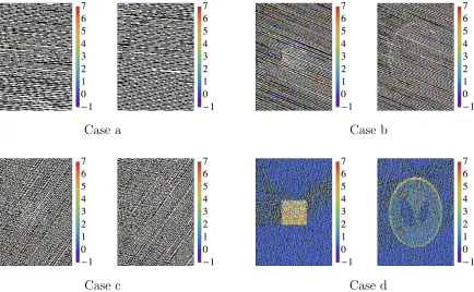
7.2 Phantoms in experiments 1, 3, 4 and 5 . . . 62

7.3 Simulated data with different noise levels for case (d) in experiment 1 63 7.4 Reconstruction without noise in experiment 1 . . . 63

7.7 Reconstruction with noise W0 = 4×104 and different regularization

parameters . . . 66

7.8 Phantom 1 in experiment 2 . . . 68

7.9 Phantom 2 in experiment 2 . . . 69

7.10 Reconstruction without noise in experiment 2 . . . 69

7.11 Reconstruction with noise in experiment 2 . . . 70

7.12 Reconstruction without regularization in experiment 3 . . . 72

7.13 Reconstruction with regularization in experiment 3 . . . 73

7.14 Reconstruction with total variation regularization for different noise levels . . . 74

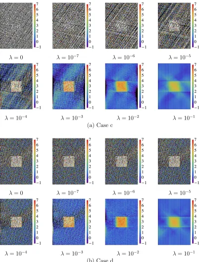
7.15 Reconstruction with total variation regularization for W0 = 4×104 and different regularization parameters . . . 75

7.16 Cross sections of reconstruction with total variation regularization for W0 = 4×104 and different regularization parameters . . . 76

7.17 Reconstruction withL1 _{regularization for different noise levels . . . 78}

7.18 Reconstruction withL1 _{regularization for W} 0 = 4×104 and different regularization parameters . . . 79

Chapter 1

Introduction

In medical imaging, absorption and scattering are two major factors that affect

the data. Different models that describe the propagation of photons are developed

during last decades. Models need to be carefully chosen according to the problem.

The problem is usually described by its scale compared to the mean free path of

the photons [30].

The most widely and successfully used technology is computerized

tomogra-phy (CT). CT reconstructs the attenuation in the medium that X-rays penetrate

through, to provide tomographic images. In CT, scattering is neglected in the

model, therefore the propagation of photons is described as straight lines.

Mathe-matically, the projection data of CT are line integrals in 2-D plane. The

reconstruc-tion procedure can be considered as inversion of an integral transform consisting of

transform.

CT can provide high-contrast images with speed and accuracy, but it also has its

limitations. One main limitation of conventional CT is that it can not be applied to

low-absorption high-scattering medium. Even in low-scattering medium, artifacts

caused by scattering affect the image of CT. Therefore, techniques are needed to

remove artifacts from the reconstruction [18]. Moreover, CT requires 180 degrees of

data collection, due to the requirement of inverting Radon transform, which limits

the size of the examined object. One more issue of concern is the radiation dose [15].

CT is regarded as a moderate- to high-radiation technique, which might increase

risk, especially when repeated tests are needed.

For higher scattering medium, models with scattering need to be taken into

account. A mathematical model for describing photon propagation with scattering

is radiative transfer equation (RTE). In RTE, radiance is defined as energy flow per

unit normal area per unit solid angle per unit time. Green’s function is essential for

analytically solving RTE, but the solution can only be obtained for simple cases.

Frameworks for solving RTE is given for different geometries [1, 5, 11, 23, 24, 32]. In

tomography, we need to solve inverse radiative transfer problem. Inverse source

problems and inverse boundary-condition problems with RTE are studied in [10,

33]. Solving the equation numerically is computational expensive, because radiance

depends on position, direction and time, which contains six different independent

For strong scattering medium, a widely used approximation for RTE is

diffu-sion approximation. A modality of medical imaging that has been developed is

diffusion optical tomography (DOT), which utilize visible light as source instead

of X-ray. It is applicable to breast imaging, and can be used to monitor brain

function and pathological changes [4, 9, 16]. In diffusion approximation, the

prop-agation of light can be described with a photon diffusion equation. However, the

diffusion approximation can only be applied to medium where scattering coefficient

is much larger than absorption coefficient, It’s not applicable near the source or

surface, with highly directed light, or in biological tissue that scatters light strongly

in forward direction. In these situations, more complicated approximation may be

required. Moreover, the inverse problem to the diffusion equation is ill-posed due

to the physics of the propagation.

Reconstruction on diffusion approximation for highly absorbing media with

col-limated sources are studied in [34, 38]. A generalized model is provided for both

steady-state and frequency-domain, which is suggested to give accurate solution

to both low and high scattering media, and also have the capacity to predict the

transition from the highly anisotropic light distribution near the collimated light

source to the isotropic light distribution in the far field. Therefore, it may be

ap-plicable to turbid medium with high absorption, and medium close to the source.

These studies suggest that generalized methods may be able to overcome some of

Another approach in DOT is higher-order approximation. PN approximation

is one of these techniques. In PN approximation, RTE is expended into spherical

harmonics and truncated at order N. When N = 1, P1 approximation gives us the

photon diffusion equation in diffusion approximation. Higher order approximation

models the anisotropy in the radiation more accurately [3, 19–21]. In application,

High-order equation is suggested to be able to applied to regions, such as

cere-brospinal fluid (CSF), which the first-order equation fails to describe, and it’s also

suggested to provide possibility to prevent the ill-posedness in solving the parabolic

equation in first-order approximation [21].

Coupled model combining RTE and diffusion approximation is proposed to

over-come the limitations when utilizing the two approaches alone [35,36]. In this model,

RTE is used in domains that assumption of diffusion is invalid, including proximity

of the source and boundary, and diffusion approximation is used elsewhere.

Nu-merical results are obtained with finite element method, and show that the coupled

model describes photon migration in low-scattering and non-scattering medium

bet-ter than only using diffusion approximation.

The model describing scattering in this thesis is on another direction from

radia-tive transfer. We focus on a weak scattering medium, and makes a single scattering

assumption. The medium should has less scattering than that for diffusion

ap-proximation and RTE, and has more scattering than that for CT. This assumption

conventional CT. It introduces new geometries that avoid the restriction of object

size, and also provides opportunity to recover scattering and absorption coefficients

of the medium.

Theoretically, in SSOT, Radon transform can be generalized to circle [7]

parabo-las [25], and also to a more general cparabo-lass of curves [8]. Compton scattering

tomog-raphy is designed to recover the local Compton-scattering cross section. The ray

is emitted and collected from one side of the object. This geometry does not

re-quire 180o access as required in CT, therefore it has the potential to utilize it for

internal structure of large objects. In this modality, attenuation due to absorption

is neglected and the measurements are related to the weighted integrals of

elec-tron density along circular arcs. An analytical solution to the inverse problem is

provided, which is analogous to the convolution backprojection algorithm used in

conventional CT [28]. A more general family of circular-arc Radon (CAR)

trans-forms is defined in [27]. The inversion of CAR is presented, which is described as

rapid and restricted to an adjustable reduced volume in order to meet the need

for imaging of smaller objects in non-destructive industrial testing, as well as in

medical imaging.

Here, instead of circles or other smooth curves, we are interested in a class of

more simple curves : piecewise line segments. In [37], three types of V-line

trans-forms are defined on a curve formed by a pair of half-lines forming the vertical letter

reconstruction algorithm is also provided for the V-line transform [26].

In [12], broken-ray Radon (BRT) transform is derived by single scattering

ap-proximation to the radiative transport equation (RTE) for known scattering

coef-ficient. BRT is defined on curves formed by a pair of half-line segments. BRT can

be considered as a generalization of V-line transform, but it does not require the

half-line segments to be symmetrical about vertical axis. The inverse problem can

be solved by discretizing the integral equations. Numerical experiment shows that

the inverse problem is only mild ill-posed. An analytical inversion formula involving

second order derivatives is derived in [14], which is analogous to filtered

backpro-jection formula. In [14], a method for separate reconstructions of absorption and

scattering coefficients is suggested. Numerical result shows that image quality is

relatively low for discontinuous attenuation coefficient, which also confirms the mild

ill-posedness of inverting broken-ray Radon transform.

Approaches to invert BRT through only first order derivatives are developed

recently. Using the measurement of three detectors and only one source,

recon-struction could be done by a method that involves only first order derivatives of

the data. This method is local and does not require a complete data set, so that

it provides more freedom in source-detector arrangement. The range of the BRT is

also described [22].

In this research, we further develop the methods of [12–14]. We focus on the

em-ployed but no energy resolution or sensitivity is assumed. We also assume scattering

occurs in the entire domain therefore the complete data can be collected. In [12],

reconstruction for BRT of a single broken-ray is studied. However, the problem is

ill-posed and reconstruction without regularization is unstable, therefore high level

regularization is needed for that method.

In this thesis, we define star transform that includes more than one

broken-rays, which will be discussed further in the next chapter. Analysis shows that it

introduces a less ill-posed inverse problem. Numerical experiments also suggest that

the reconstruction is more stable than the one with only one broken-ray. Recovering

scattering and absorption coefficients simultaneously is also studied in this thesis.

The reconstruction is theoretically feasible and the numerical experiments also show

stable results. Experiments with more realistic simulated data are needed for future

research.

However, the results in our numerical experiments are susceptible to noise. In

order to have better results, we can include data of the ballistic rays, which can be

collected simultaneously when the scattered data is measured. Without scattering,

data of ballistic ray is supposed to have higher intensity and have less noise, therefore

we expect the additional data provided by ballistic rays can help reduce the effect

of the noise from the data of scattering rays.

The techniques of SSOT mentioned before do not involve ballistic ray in the

provides opportunity to apply SSOT for medium with lower scattering. CT requires

180o projection data of ballistic rays to perform reconstruction, but a full collection

of ballistic data may be impossible in SSOT models. However, with the limited

ballistic data we are able to collect, we can find reconstruction of SSOT that is

consistent with it, without significant change to the image reconstruction procedure.

In this thesis, we derive an algorithm in Fourier domain to find the reconstruction

consistent with the ballistic data, by only a minor adjustment to the inversion

algorithm for star transform. We expect including ballistic ray to be an effective

improvement to our model.

Other approaches to improve the image quality is utilizing different

regulariza-tions. Tikhonov regularization is added during the procedure of reconstruction to

overcome the ill-posedness of the inverse problem, but it does not provide good

im-age when noise level is high. We present algorithms to implement the total variation

regularization andL1 regularization. These two regularizations can help remove the

Chapter 2

The problem

2.1

Geometry

In single scattering tomography, image reconstruction can be performed for 3-D

medium by reconstructing 2-D images slice by slice. In each slice, the problem is

reduced to a 2-D problem. Therefore, in this thesis we only focus on the problem of

2-D reconstruction. Suppose the domain for imaging is a 2-D slice of a 3-D medium

with X = const. The geometry of this slice is an open strip _S = {0 < z < L} as

shown in Figure 2.1, which is assumed to be infinitely long in direction of Y-axis.

In contrast to conventional CT, which assume that no scattering occurs, we

as-sume that the majority of incident photons undergo single scattering in the medium.

To be specific, we require the width L of the strip along the Z-direction to match

The reconstruction is designed based on this assumption.

Suppose a photon incident from one side of the strip undergoes a single scattering

and its direction changes. The propagation trajectory is a broken line. The power

of the incident ray attenuates along the trajectory, which is caused by two major

factors : absorption and scattering. The strength of absorption and scattering at

location R is described by absorption coefficient µa(R) and scattering coefficient

µs(R). These two coefficients vary inside the medium, so they can be considered as

two non-negative functions spatially distributed on _S. The attenuation coefficient

is the sum of the previous two :

µ(R) =µa(R) +µs(R). (2.1.1)

We will focus on reconstructing function µ(R) first, and recover µa(R) and µs(R)

in the next step.

The data for this problem is obtained in the following way: sources that emit

photons are aligned on one side of the strip. On the other side of the strip, we have

angularly fixed collimated detectors, which only collect signals of rays with certain

outgoing directions. Suppose a photon is sent into the medium at the location Y1

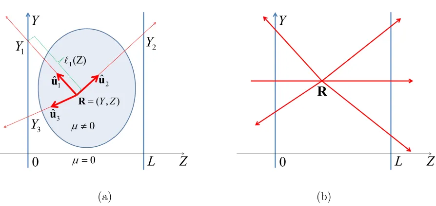
with direction ˆu1, and it’s received at location Y2 with direction ˆu2. Each pair of

(Y1, Y2) determines a broken line as shown in Figure 2.2. The vertex of the broken

line, R = (y, z), is where scattering occurs. Suppose the directions ˆu1 and ˆu2 are

ˆ

u2 = (u2y, u2z), R = (Y, Z), the coordinates of R and (Y1, Y2) have the following

relation,

Y1 =Y − u1y

u1z

Z , Y2 =Y − u2y

u2z

(L−Z) . (2.1.2)

Therefore, the data can also be considered as a function of R. We denote the data

collected at Y2 by W(R). The goal of single scattering tomography is to recover

µ from W. We assume that scattering coefficient is strictly positive everywhere in

the medium: µs(R) > µ¯s > 0 for every R ∈ S¯. In order to have W(R) exist on

the entire domain _S, it is important to have this assumption. Otherwise, W(R)

does not exist because no scattering occurs at R. Here ¯µs is a positive constant

indicates the scattering strength on the background. This assumption also implies

that µ(R)>µ¯s >0 in S. W0 and W have the following relation,

W(R) =W0S12µs(R) exp{−[I1(R) +I2(R)]} , (2.1.3a)

Ik(R) =

Z `k(R)

0

µ(R+ ˆuk`)d` , k = 1, 2. (2.1.3b)

Here `k(R) is the value that R+ ˆuk`k(R) = 0, orL, depending on the sign of ukz.

S12 is the phase function describing the geometry, which only depends on ˆu1 and

ˆ

u2. It’s determined when the directions are fixed. W0 and S12 are both assumed to

be known constants. We define the signal function Φ by taking logarithm of W,

Φ(R) = −log

W(R)

W0S12µ¯s

Φ(R) is the integral of µ along a broken line, plus a term involving scattering

coefficient µs(R). If µs is a known constant in the medium, Φ(R) only involves

integral ofµ. However, whenµsis not constant, the problem involves both functions

µandµs. We’d like first removeµs from (2.1.4), so we can turn the problem into an

inverse integral problem for µ. The method to remove µs is to utilize more signals.

Suppose we have K fixed vectors ˆuk, k = 1, . . ., K. Each vector can be an

incident direction or an outgoing direction of the rays, or both. Each pair of them

defines a collection of data, so we totally have K(K−1)/2 data: Wij,i, j = 1, . . .,

K,i6=j. Wij is the data corresponding to ˆui and ˆuj. Figure 2.2 (a) shows the case

for K = 3. The signal function introduced by Wij(R) is:

Φij(R) = −log

Wij(R)

W0Sijµ¯s

=Ii(R) +Ij(R)−log [µs(R)/µ¯s] . (2.1.5)

All signal functions have three terms, the first two of them are line integrals

of µ. The third term which contains µs(R) is shared by all signal functions. This

term can be canceled by adding up these functions with weighted factors. We

choose coefficients cij, i, j = 1, . . . , K, i6=j, such that

P

i6=jcij = 0, and define

coefficients si =

P

gives us a system of equations without scattering coefficient involved :

Φ(R) = X

i,j

cijΦij(R)

=X

i,j

cij[Ii(R) +Ij(R)−log (µs(R)/µ¯s)]

=X

i

X

j6=i

cijIi(R)−

X

i6=j

cijlog (µs(R)/µ¯s)

=

K

X

i=1

siIi(R).

(2.1.6)

We define (2.1.6) to be star transform with K branches:

Φ(R) =

K

X

i=1

siIi(R) , Ik(R) =

Z `k(R)

0

µ(R+ ˆuk`)d` . (2.1.7)

The star transform can be well defined for function in L1₍

S). In the next chapter,

Figure 2.1: A broken line incident at Y1 in ˆu1, scattering at R, outgoing at Y2 in ˆ

u2.

2

ˆ

u

1

ˆ

u

( , )_{Y Z}

R

Z

L

0

Y

3

ˆ

u

0

!"

1(Z)

1

Y

Y

3

Y

0

!

0

_L

_Z

Y

R

(a) (b)

Chapter 3

Inversion of the star transform

In this chapter, we turn to the problem of inverting star transform. An simple idea

to find the inverse is discretizing the transform. However, attenuation coefficient and

the signal function are both 2-D functions, so the computation complexity would be

large. Suppose the domain is discretized into N×N grid, the problem would have

N2 equations of size N2. This will be infeasible in numerical aspect. Moreover, it’s

difficult to analyze the stability and add regularization in that approach. In this

thesis, we will present an approach to find the inverse in Fourier domain.

3.1

The star transform in Fourier domain

We assume that attenuation coefficient µ inside the medium is compactly

sup-ported, so Fourier transforms of Φ and µare well defined. First, we introduce some

Fourier transform: F : S(_S)→S(_S) (3.1.1a)

Inverse Fourier transform: F−1 : S(_S)→S(_S) (3.1.1b)

Star transform: F : L1(_S)→L1(_S) (3.1.1c)

HereS(_S) is the Schwarz space on _S, which is a subspace ofL1₍

S). The

recon-struction procedure is

Φ−−−−−−→F Φn(q)

Inverse problem in Fourier domian

−−−−−−−−−−−−−−−−−−−−→µn(q) F

−1

−−−−−−−→µ .

We first compute Fourier transform of Φ and then solve the inverse problem in

Fourier domain. Finally, taking inverse transform gives us the attenuation

coeffi-cient µ. The Fourier transform is defined as

µ(y, z) =

Z ∞

−∞

dq

2πe

iqy_{µ˜(q, z) =}

Z ∞

−∞

dq

2πe

iqy1

L

∞ X

n=−∞

µn(q)eiκnz , (3.1.2a)

µn(q) =

Z ∞

−∞

dye−iqy

Z L

0

dze−iκnz_{µ(y, z), (3.1.2b)}

κn =

2πn

L . (3.1.2c)

In (3.1.2), q is the Fourier parameter corresponding to y, and κn is the parameter

unbounded in Y-direction, this is the reason that the definition of our Fourier

transform differs in Y and Z directions. To find the relation between Φn(q) and

µn(q), we start by taking Fourier transform (2.1.7) with respect toY:

˜

Φ(q, Z) =

K

X

k=1 sk

Z `k(Z)

0

d`

Z ∞

−∞

µ(Y +uky`, Z +ukz`)eiqYdY

=

K

X

k=1 sk

Z `k(Z)

0

e−iquky`<sub>µ˜(q, Z+u</sub> kz`)d`

= K X k=1 sk ukz

e−iβk(q)Z

Z ξk

Z

eiβk(q)z_{µ˜(q, z)dz}

= K X k=1 sk ukz

e−iβk(q)Z

Z ξk

Z

eiβk(q)zX m

µm(q)eiκmzdz

= K X k=1 sk ukz

e−iβk(q)Z ∞ X

n=−∞

ei[βk(q)+κn]ξk−_ei[βk(q)+κn]Z

i[βk(q) +κn]

µn(q) . (3.1.3)

In the above derivation, we have used the fact that the upper limit of integration

over `, `k(Z), is independent of Y. The notations in (3.1.3) are defined as

βk(q) = q

uky

ukz

, ξk =

      

L , if ukz >0

0, if ukz <0

. (3.1.4)

Hereξkis theZ-coordinate of thek-th ray intersection with the boundary ofS. Since

we assume that all rays intersect the strip boundaries, the quantities in (3.1.4) are

well defined. We also have that exp(iξkκn) = 1 for all k.

To shorten the notations, we will omit the parameter q in (3.1.3) below by

of (3.1.3) with respect to Z, which results in the following infinite system of linear

equations:

Φn =µn K

X

k=1

isk

ukz(βk+κn)

+

K

X

k=1

skeiβkξk e−iβkL−1

Lukz(βk+κn)

∞ X

m=−∞

µm

βk+κm

. (3.1.5)

Introducing notations

dn= K

X

k=1

isk

ukz(βk+κn)

= K X k=1 isk ˆ

uk·(q, κn)

, αk =

eiβkξk _e−iβkL−₁

Lukz

, (3.1.6)

we can rewrite (3.1.5) in the form

Φn=dnµn+ K

X

k=1

skαk

βk+κn

∞ X

m=−∞

µm

βk+κm

. (3.1.7)

Furthermore, (3.1.7) can also be written in matrix form:

Ax=Dx+

K

X

k=1

The matrices and vectors are defined as

A=D+

K

X

k=1

αkaka∗k , (3.1.9a)

D =         . .. PK k=1 isk ukz(βk+κn)

. ..         , (3.1.9b)

ak =

· · · 1

βk+κn

· · ·

T

, (3.1.9c)

Φ= (· · · Φn · · ·)T . (3.1.9d)

MatrixA is a diagonal matrixD with K separable terms (Rank-1 matrix). We

can use this feature to find specific algorithm for inversion of A, with advantages

in effectiveness and stability.

3.2

Direct inversion

As defined in (3.1.7), each equation has infinitely many terms. Theoretically, an

inversion algorithm for (3.1.7) exists. We assume D in equation (3.1.8) to be

in-vertible. Multiplying the equation from left by aj∗D−1, gives us

yj+ K

X

k=1

where yj, Mjk and zj are defined as

yj =aj∗x, Mjk =αkaj∗D−1ak , zj =aj∗D−1Φ. (3.2.2)

Although (3.1.7) has infinitely many equations and unknowns, (3.2.1) has only K

equations with K unknowns. Suppose variables in (3.2.2) are well defined, the

system of equations is of a small size K, which can be easily solved. Then the

solution xcan be computed by

x=D−1Φ−

K

X

k=1

αkykD−1ak . (3.2.3)

Dis a diagonal matrix, (3.2.3) can be computed entry by entry. To be more specific,

the nth entry in (3.2.3) is

xn=dn

−1 Φn−

K

X

k=1

αkykdn

−1

akn . (3.2.4)

One issue needed to be discussed before using (3.2.3) is whether variables in

(3.2.2) are well defined. The variables are defined as sum of infinitely terms, so we

need to guarantee those sums converge. Let’s first consider Mjk,

Mjk =αk

∞ X

n=−∞

1

dn(βj +κn)(βk+κn)

. (3.2.5)

1

βj +κn

can be expended as

1

βj +κn

= κn−1(βj/κn+ 1)

−1

= κn−1

1−βjκn−1+βj2κn−2+O(κn−3)

= κn−1−βjκn−2+βj2κn−3+O(κn−4).

(3.2.6)

Then the following functions can also be expended into series with respect to κn−1,

1

(βj +κn)(βk+κn)

=κn−2−(βj+βk)κn−3+O(κn−4) , (3.2.7a)

dn=t1κn−1−t2κn−2 +O(κn−3) , (3.2.7b)

dn

−1

=t1−1κn+t1−2t2+O(κn−1) , (3.2.7c)

where the notations are

t1 =

K

X

k=1

isk/ukz , t2 =

K

X

k=1

iskβk/ukz .

odd n are canceled. t1, t2 are independent with n, so

Mjk =

1

βjβkd0

+P

n6=0{t1κn

−1_{+ [t}

1−2t2−t1(βj +βk)]κn−2+O(κn−3)}

= 1

βjβkd0

+P∞

n=1{[t1

−2_t

2−t1(βj+βk)]κn−2+O(κn−4)} .

(3.2.8)

κn∼O(n), so the sum in (3.2.8) converges. Mjk are well defined. Next we turn to

zj =aj∗D−1Φ. Using the result in (3.2.7), the nth entry of aj∗D−1 is

aj∗D−1

n=t1

−1_+O(κ

n−1) . (3.2.9)

(aj∗D−1)_n is bounded. Φis the Fourier coefficients of signal function, so P_nΦn <

∞. Therefore zj = aj∗D−1Φ < ∞ is also well defined. In this section we have

presented a direct method that is theoretically applicable for even infinite system.

In practice, we need to truncate the Fourier series to have a finite system. In the

next section, we will talk about an approach to compute the numerical inverse of

A with truncation, which is used in the simulation chapter in this thesis.

3.3

Inversion of star transform in Fourier domain

In this section, we will introduce an iterative method to compute the inverse of

(3.1.7). Here we assume the data is discretized on a N×N grid. Then the matrix

A is N ×N, and the vectors in (3.1.9) are N ×1. Before considering inverting

Let this matrix A be

A=D+ba∗ . (3.3.1)

Dis aN×N diagonal matrix,aandbare bothN×1 vectors. The inversion formula

is derived from Sherman-Morrison formula. We first assume D to be invertible, to

be specific, all diagonal entries ofD are not zero. We also assumeD to be nonzero,

which is defined as

D = 1 +a∗D−1b . (3.3.2)

When the two assumptions hold, the inversion formula is given by

T =D−1ba∗ , A−1 =D−1−D−1TD−1 . (3.3.3)

Requiring |D|>0 is essential because the determinant of A is given by

|A|=D |D| =D

N

Y

n=1

dn . (3.3.4)

So the two assumptions above are actually equivalent to A is invertible. When

utilizing this formula in numerical computation, a small singular value of D or a

small |D| can lead to unstable result. Therefore, we need more strict conditions.

We require |D| > σ, where σ > 0 is some pre-selected small constant. Formula

(3.3.3) is only applicable to invertible A, but in some case evenA is not invertible,

, the inverse of D is

D−1 =Dreg−1+

1

vw

∗

, v∗Dreg =Dregw= 0 . (3.3.5)

vand ware the singular vectors corresponding to singular value 1/in the singular

value decomposition (SVD) of D−1_{. Plugging (3.3.5) to (3.3.3), and taking → 0,}

it gives us a formula for inverting A,

A−1 =Dreg + D reg

a∗_vb∗_wvw ∗₋ 1

a∗_vva ∗

Dreg−1−Dreg−1bw∗

1

w∗_b , (3.3.6a)

Dreg = 1 +a∗Dreg−1b . (3.3.6b)

We can use (3.3.3) when D is invertible, or (3.3.6) when it has a small singular

value. In both cases, the inversion for matrix with one separable term is simple to

compute. Notice that (3.3.3) and (3.3.6) only involve the inverse of D, so they are

applicable as long as we know the inverse of D, even D is not diagonal.

We can generalize this algorithm for the matrix with K separable terms, by

repeating (3.3.3). Suppose we have a matrix

A =D+

K

X

i=1

biai∗ . (3.3.7)

(3.1.8), we have bi = αiai. We will introduce more notations. Let Ak be the

matrix with the first k separable terms, k ≤K,

Ak =D+ k

X

i=1

biai∗ , k = 0, · · · , K . (3.3.8)

The two special cases are A0 = D and AK = A. We start with inverting A0

and iteratively calculate the inverse of Ak for k = 1, 2 , . . . , K. When Ak−1 is

obtained, we use (3.3.3) to compute the inverse of Ak+1. This is a direct method,

because we are guaranteed to find the inverse of A when the algorithm terminates

after K steps. The iteration in detail is

• First iteration step. Assume that D has no small singular value or only one

small singular value, otherwise the algorithm is not applicable. Then start

with A0 =D and consider the first step of iteration, A1 =A0+b1a1∗.

• Iteration step. Assume that A−_k1 is obtained for some k < K. Compute the

determinant

Dk = 1 +ak+1∗Ak−1bk+1. (3.3.9)

If|Dk|< σ, where σ is a pre-selected small constant, iteration is theoretically

feasible, but numerically unstable. Otherwise, compute the k-th update of

the matrix according to

Next, compute Ak+1−1 according to

A−_k+11 =A−_k1−A−_k1TkA−_k1 , (3.3.11)

and move to the next iteration step.

• Termination. The procedure is terminated after K iterations and converges

to A−1 _=A

K−1 as long as all determinants Dk (k = 1,2, . . . , K −1) satisfy

the condition |Dk|> σ.

For this algorithm to be feasible, we assume that all|Dk|>0. Similar to the case for

K = 1, |Dk|>0 is equivalent to Ak is invertible. Therefore we have a more strict

requirement for A: not only A needs to be invertible but also all the intermediate

Ak.

3.4

The special case for

q

= 0

In the last section, we omit a fact: when q = 0, all βk in (3.1.4) are zero, so D,

bk, ak are not well defined because all entries withq = 0 are infinite. Therefore we

the derivation of (3.1.3). The equations that we obtain are different from (3.1.7),

˜

Φ(0, Z) =

K

X

k=1 sk

Z `k(Z)

0

d`

Z ∞

−∞

µ(Y +uky`, Z +ukz`)dY

=

K

X

k=1 sk

Z `k(Z)

0 ˜

µ(0, Z+ukz`)d`

= K X k=1 sk ukz

Z ξk

Z

˜

µ(0, z)dz

= K X k=1 sk ukz X

n6=0

1−eiκnZ

iκn

µn(0) + (ξn−Z)µ0(0) !

. (3.4.1)

Applying Fourier transform with respect toZ to ˜Φ(0, Z), and takingeiκnL _{= 1 into}

account, equation (3.1.7) becomes

Φn=iΣ1

µn−µ0 κn

, n6= 0 , (3.4.2a)

Φ0 = LΣ0

2 µ0−i X

m6=0 Σ1 κm

µm , (3.4.2b)

where the constants Σ0 and Σ1 are

Σ0 =

K

X

k=1 sk

|ukz|

, Σ1 =

(3.4.2) is much simpler than (3.1.7). Suppose |Σ0|>0 and |Σ1|>0, (3.4.2) can be

solved with

µ0 = 2

LΣ0 X

m

Φm , (3.4.4a)

µn=µ0−i κnΦn

Σ1

. (3.4.4b)

This algorithm is not only applicable for truncated equations, but also for the direct

method with infinite system of equations. In the later one, the term P

mΦm equals

to ˜Φ(0,0). The value of Σ0and Σ1depend on the directions of ˆukand the coefficients

sk. We need to prevent them to be too small when choosing ˆuk.

3.5

Pseudo-inverse of star transform in Fourier

domain

In the last section, we have discussed an algorithm for inverting (3.1.7). The

algo-rithm works whenAkare invertible andDkare not too small, fork = 1, 2, . . . , K.

However, for star transform we are not guaranteed to have them hold. When the

requirements are not met, we still want to reconstruct µ. We can compute the

pseudo inverse and add regularization. The pseudo inverse of a matrix A is defined

as

Pseudo inverse of a matrix is widely used in solving linear least-square problem,

or finding the minimum norm solution to s linear system. For pseudo inverse, we

don’t needAto be invertible or even square. Hereλis the regularization parameter.

When A is invertible and λ→0, the pseudo inverse converges to the inverse A−1_,

so pseudo inverse is an extension of conventional inverse. A†x is the minimizer of

the optimization problem

min

x kAx−Φk

2_+λkxk2 _{. (3.5.2)}

For single scattering tomography, we assume that the number of detectors is no less

than the image resolution, so we have on less equations than unknowns. It means

that the matrix has more rows than columns. For a N ×M matrix A (N ≥ M),

we define two matrices to help compute pseudo-inverse. One is of size N ×N and

the other is M ×M. The two matrices are defined as

SN = (AA∗+λIN)−1 , (3.5.3a)

SM = (A∗A+λIM)−1 . (3.5.3b)

HereIN andIM are the identity matrices of the size N×N andM×M respectively.

SN and SM are well defined when λ >0. Then the pseudo inverse ofA is given by

A†=SMA∗ =A∗SN. We will introduce an algorithm similar to the one in Section

step. We first introduce some notations:

SN,k = (AkA∗k+λIN)−1 , (3.5.4a)

SM,k = (A∗kAk+λIM)−1 . (3.5.4b)

These matrices correspond to the pseudo inverse of Ak defined in (3.3.8). The

iteration starts with computing SN,0 and SM,0. For λ >0, even D is singular, SN,0

and SN,0 are well defined. In the case of Star transform, SN,0 and SM,0 are diagonal

matrices with the diagonal entries

sm =

1 |dm|2+λ

, m = 1 , 2 , · · · , M . (3.5.5)

In the case N > M , the matrix SN,0 has sm as the first M diagonal entries and

1/λ2 _{as the lastN−M entries, while S}

M,0 is theM×M minor ofSN,0. Compared

to the case in computing inverse in Section 3.3, we also need two matricesTN,k and

TM,k, instead of only one Tk. The main iteration step is

SN,k+1 =SN,k−SN,kTN,kSN,k , (3.5.6a)

SM,k+1 =SM,k−SM,kTM,kSM,k , (3.5.6b)

Here TN,k and TM,k are updated with

TM,k =

1

Dk

h

γkak+1bk+1∗Ak+ H.c.

+λ2Qkak+1ak+1∗−PkAk∗bk+1bk+1∗Ak

i

, (3.5.7a)

TN,k =

1

Dk

h

γkAkak+1bk+1

∗

+ H.c.

+λ2Pkbk+1bk+1∗−QkAkak+1ak+1∗Ak∗

i

, (3.5.7b)

where ”H.c.” stands for Hermitian conjugate of the preceding term and

γk = 1 +ak+1∗Ak†bk+1 , (3.5.8a)

Pk =ak+1∗SM,kak+1>0 , Qk =bk+1∗SN,kbk+1 >0, (3.5.8b)

Dk =|γk|2+λ2PkQk >0 . (3.5.8c)

Here ak is M ×1 vector and bk is N ×1 vector. This iteration terminates when

k = K, and A† = ASN,K = SM,KA. Computing the pseudo inverse is more

complicated than computing the inverse. The basic requirement is Dk > 0. The

analysis of complexity and stability is needed to be studied carefully and it will be

Chapter 4

Analysis of the algorithms

4.1

Computational complexity

One advantage of the two algorithms in the last chapter is computational

effec-tiveness. Suppose the domain _S is discretized into a N ×N grid. For each

sys-tem of equations in form (3.1.7), the size of A is N ×N. When computing the

inverse A−1_{, using the algorithm mentioned above is faster than Gaussian}

Elimi-nation, which takes only O(N3_{) computation. The first iteration step is computing}

A0−1, which is simple because A0 = D is a diagonal matrix. When updating

Ak+1−1 according to (3.3.11), we don’t compute the product of Ak−1TkAk−1

di-rectly. We first compute Ak−1bk+1 and Ak−1ak+1, then compute Ak−1TkAk−1 =

D−1_(A

k−1bk+1)(Ak−1ak+1)∗. So we only need to compute product between a

can also be broken into product between matrix and vector, therefore the

compu-tational complexity for each iteration step is O(N2) and the total complexity for

solving each system of equations by this algorithm is O(KN2_{). For star transform,}

K N (In our simulation experiments, we use K = 3), so the complexity is much

less than O(N3).

The case for computing pseudo inverse is similar. When computingSN,kTN,kSN,k

and SM,kTM,kSM,k, we can always use the definitions of TN,k and TM,k to break

them into product of vectors, then all computation are between matrices and

vec-tors. Although the algorithm in computingA†is more complicated than computing

inverse, but we don’t need to compute product between matrices. The complexity

is also O(KN2) for solving each system of equations.

For the reconstruction, we haveN systems of equations, so the total time needed

is O(KN3_{). We should also take the computation for Fourier transform into}

ac-count. The computational amounts for 2-D Fourier transform and inverse Fourier

transform areO(N2_{logN) when utilizing Fast Fourier Transform (FFT). Therefore}

the total computational amount needed is O(KN3_{). For comparison, suppose we}

discretize star transform (2.1.7) directly, the number of equations and unknowns

are both N2_{, therefore the size of the problem is N}2_{. Using Gaussian Elimination}

to solve the problem takes computation as much as O(N6_{). So the complexity for}

4.2

Stability

Another issue needed to be considered is the stability of the algorithms. The

com-puting of the inverse is stable only if diagonal matrix D is stably inverted. For a

fixed parameter q, the entry of D is defined in (3.1.9). Let’s write the nth entry

dn(q) in the form of

dn(q) = K

X

k=1

isk

ˆ

uk·(q, κn)

= i

|(q, κn)| K

X

k=1 sk

uk·vˆ

, (4.2.1)

where ˆv= (q, κn)/

p

q2 _+κ2

n is a unit vector pointing to the direction of (q, κn). We

can consider dn(q) as a function of (q, κn). If there exists some (q, κn) such that

dn(q)≈0, it leads to instability when inverting D. Define function

f(θ) =

K

X

k=1

sk

cos(θ−θk)

=

K

X

k=1 sk

uk·vˆ

, (4.2.2)

where θ and θk are the angles of ˆv and ˆuk with the positive direction of Z-axis.

dn(q) = 0 for some (q, κn) if and only if f(θ) = 0 for some θ. One thing needs to

mention is that f(θ+π) = f(θ), therefore, it is sufficient to consider the interval

0 ≤ θ < π. Suppose f(θ) has a zero point ˜θ in [0, π), then for (q, κn) with angle

close to ˜θ, the entry dn(q) would be very small. We expect f(θ) to have no zeros,

so we can prevent the singularity of D.

We have found necessary conditions for f(θ) has no zero: (i) First, K needs

in Y Z plane. Before we prove that these are necessary conditions, we first clarify

some facts about f(θ). Let ηk,± denote θk ±π/2. Notice that f(θ) → ∞ when θ

goes to ηk,± (In geometry, this is when ˆv is perpendicular to ˆuk), so ηk,± are the

singular points of f(θ). Between two adjacent singular points, f(θ) is a continuous

function. Therefore, between two adjacent ηk,±, iff(θ)→ ∞with different signs as

θ approaches to the two ends of the interval, there is at least one zero point inside

the interval. Another thing worth noticing is the signs of sk cos(θ−θk)

are different

inside (ηk,−, ηk,+) and outside this interval. Therefore, for each η =ηk,±, f(θ) has

different signs in interval (η−, η) and (η, η+), whereis an infinitesimal constant.

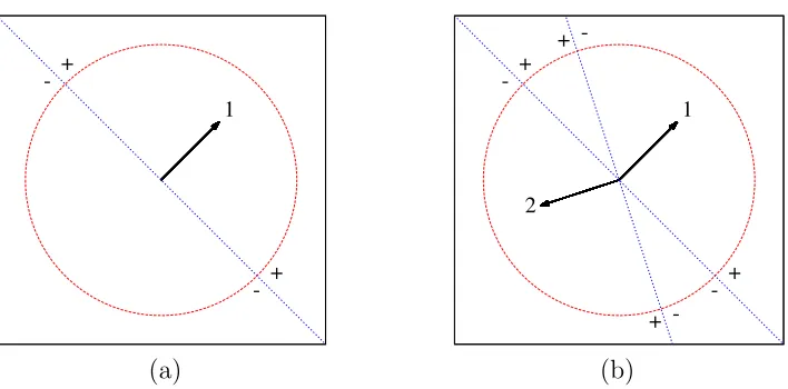
With all the observations above, we can show the two conditions mentioned

above are necessary. Let’s place skuˆk onto the plane one by one. The first unit

vectors1uˆ1can be placed on the plane arbitrarily, and its perpendicular line divides

[0,2π) into two intervals as shown in Figure 4.1 (a). In the figure, we use a circle

to indicate [0,2π) and the two half circles are the two intervals divided by the

perpendicular line of ˆu1. In each of this interval, f(θ) has the same sign near the

boundary of the interval. This is also easy to see from the formula of f(θ) with

K = 1. When adding the second vectors2uˆ2, supposes2uˆ2 has a different direction

with s1uˆ1, each of the half circles is divided into two. No matter how we place

the second vector, there must be two intervals in which f(θ) changes sign. This

is shown in Figure 4.1 (b). So f(θ) must have zero points for K = 2. Suppose

in the interval with different signs, we have a chance to prevent the appearance of

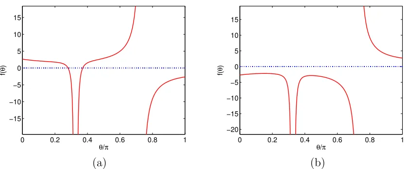
the intervals in which f(θ) has different signs. Figure 4.2 can help us prove this.

Suppose we already have two vectors placed in the plane. As discussed above, now

[0,2π) is divided into four intervals, in two of which f(θ) have the same sign near

boundary and in the other two f(θ) have different signs. If we want f(θ) have the

same sign near boundary in all intervals after putting s3uˆ3,θ3±π/2 must be placed

in the intervals in which f(θ) changes sign, like the case in Figure 4.2 (a). In this

case, the angles between any two adjacent skuˆk are less then π/2. Otherwise, as

shown in Figure 4.2 (b), there must be an interval in which f(θ) changes sign, so

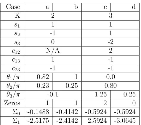
f(θ) have zero points in this interval. Figure 4.3 is the plot of f(θ) corresponding

to Figure 4.2, we can see when conditions (ii) is not satisfied, f(θ) has zeros. This

necessary condition can be generalized for K >3 in the same way.

However, even conditions (i) and (ii) are satisfied, it does not guarantee that

f(θ) has no zero. This is because evenf(θ) has the same sign near the two ends of a

interval, it can still cross the line f(θ) = 0 inside the interval. Figure 4.4 shows the

case when (i) and (ii) hold butf(θ) still has zeros. In the simulation section, we will

demonstrate that whether f(θ) has zeros is essential to the stability of inversion.

Therefore for more stable reconstruction, we need to choose ˆuk andsk to make sure

|f(θ)|> σ >0, where σ is some small constant.

1 + -+ -1 2 + -+ + + -(a) (b)

Figure 4.1: (a) Placing s1uˆ1, the unit circle is divided into two parts. (b) Placing the second vector s2uˆ2, the unit circle is divided into four parts. The labels + or

− indicates the sign of f(θ) when θ approaches the blue dash line. In Figure (b),

f(θ) has zeros in the top-right and bottom-left intervals.

1 2 3 + -+ + + -+ -+ -1 2 3 + -+ + + -+ -+ -(a) (b)

Figure 4.2: Sign diagrams for the function f(θ) in the case K = 3 and θ1 =−π/6, θ2 = 0.82π, θ3 = 0.23π. Angles are measured from the positive direction of the Z -axis, which runs horizontally from left to right. The coefficients sk are s1 =s2 = 1, s3 = 2 (a) and s1 = s2 = 1, s3 = −2 (b). It can be seen that the drawing of the third line, which goes in this case from the top left to the bottom right corner, removes the contradiction in the case (b) but not in (a). By inspection, it can be verified that in (a) all vectors skuˆk can be placed in the same half-plane while in

0 0.2 0.4 0.6 0.8 1 −15 −10 −5 0 5 10 15 θ/π f( θ )

0 0.2 0.4 0.6 0.8 1

−20 −15 −10 −5 0 5 10 15 θ/π f( θ ) (a) (b)

Figure 4.3: Plot for f(θ) in the case K = 3 and θ1 = −π/6, θ2 = 0.82π, θ3 = 0.23π. Angles are measured from the positive direction of the Z-axis, which runs horizontally from left to right. The coefficients sk are s1 =s2 = 1, s3 = 2 (a) and s1 =s2 = 1, s3 =−2 (b). f(θ) has zeros in (a) but no zero in (b).

0 0.2 0.4 0.6 0.8 1

−20 −15 −10 −5 0 5 10 15 θ/π f( θ )

Figure 4.4: Plot for f(θ) in the caseK = 3 and θ1 =−π/6,θ2 = 0.82π, θ3 = 0.23π and coefficients are s1 = 1.4, s2 = 0.6, s3 = 2. ˆuk satisfy necessary conditions (i)

guarantee Dk not to be too small, the process will be stable. We have discussed

before,Dkis the determinant ofAk, therefore the stability of reconstruction depends

on the invertibility of all Ak.

In the computation of pseudo inverse, adding regularization can help reduce the

instability. In each iteration step, since we have λ > 0, SM,k and SN,k in (3.5.4)

are both positive definite. Hence Pk and Qk in (3.5.8) are strictly larger than 0, so

Dk >0 for each step k. The computing the pseudo-inverse is stable.

To be more specific, suppose Ak = UΣV∗ is the singular value decomposition

(SVD) ofAk, we haveSM,k =V(Σ2+λ2IM)V∗. Similarly,SN,k=U(Σ2+λ2IN)U∗.

Then Pk and Qk can be written as

Pk= M

X

i=1

|(Vak)i|2

σ2

i +λ2

, Qk= N

X

i=1

|(Ubk)i|2

σ2

i +λ2

. (4.2.3)

Here (Vak)i is theith entry of Vak, (Ubk)i is the ith entry of Ubk, and σi is the

ith diagonal entry of Σ. InQk, σi = 0 fori > M. Then the second term in (3.5.8c)

is

λ2PkQk =λ2 M

X

i=1

|(Vak)i|2

σ2

i +λ2

! _N

X

i=1

|(Ubk)i|2

σ2

i +λ2

!

. (4.2.4)

SupposeAkis singular,|γk|= 0. In this case, there is someσn= 0, soDk ∼O(λ−2).

If we choose regularization parameter λ properly, we can guarantee Dk not to be

Chapter 5

Reconstruction of scattering and

absorption coefficients

In the last two chapters, we have discussed the method for reconstructing

atten-uation coefficient µ, now we turn to reconstruction of scattering and absorption

coefficients. As mentioned before, one advantage of single scattering tomography

over CT is that it provides an opportunity to recover the scattering coefficient and

also absorption coefficient. This is because in our model scattering coefficientµs(R)

is a weighted factor in signal function Φjk(R). We rewrite signal function (2.1.5) as

µs(R) = ¯µsexp [Ij(R) +Ik(R)−Φjk(R)] . (5.0.1)

Here j and k can be any two distinct numbers from 1, 2, . . ., K. Since Φjk(R) is

are Ij(R) and Ik(R). This two terms are the line integrals of µ along broken line

with vertex R. One direct way to compute Ij(R) and Ik(R) is numerical integral.

In this thesis, we compute them in Fourier domain as well, and compute the sum

Ij +Ik together instead of computing them separately. Let

ψ(R) = Ij(R) +Ik(R). (5.0.2)

The Fourier coefficients of ψ is defined as

ψn(q) =

Z ∞

−∞

dye−iqy

Z L

0

dze−iκnz_{ψ(y, z) . (5.0.3)}

Use the same method in deriving (3.1.7), the Fourier coefficients for ψ has the

relation with the Fourier coefficients of µ,

ψn=dnµn+

αj

βj+κn

X

m

µm

βj +κm

+ αk

βk+κn

X

m

µm

βk+κm

, (5.0.4)

Here βj, βk are defined in (3.1.4), and κn is the parameter defined in (3.1.2). The

matrices are the same as defined in Section 3.1. We also omit the q in the same

way in Section 3.1. This is actually a direct problem for the broken-ray Radon

transform. The Fourier coefficients of µ can be obtained during the reconstruction

transform with FFT, then we will have ψ =Ij +Ik:

µn(q)

(5.0.4)

−−−−−−−−→ψn(q) F

−1

−−−−−−→ψ .

Then µs(R) can be computed by (5.0.1). We could use any signal function Φjk to

compute µs, or we could use more than one Φjk and compute the average of the

results. After recovering µs, the absorption coefficientsµa is the difference between

µ and µs:

µa(R) = µ(R)−µs(R). (5.0.5)

In contrast to the reconstruction of µ, reconstructions of µs and µa do not

involve solving inverse integral problem. The procedure mentioned above won’t

cause instability. However, the reconstructions of µs and µa highly depend on the

reconstruction of µ.

For the aspect of computational complexity, computing Fourier coefficients of

ψ = Ij +Ik takes O(N2), and computing Fourier transform costs O(N2logN).

This approach for computing ψ takes totally O(N2_{logN). It just takes a little}

more computation for recovering scattering and absorption coefficients. This is

Chapter 6

Improving the image quality

Our imaging reconstruction assumes single scattering. If this assumption holds, it

provides us a chance to recover the scattering and absorption coefficients. However,

the scattering phenomenon also causes significant loss of the power of incident rays.

It also causes the signal to be susceptible to noise. Simulation results show that

the reconstruction suffers badly from high level noise. In this section, we will talk

about some approaches to reduce the effect of noise and improve the image quality.

6.1

Including ballistic data

The first approach is to include some less noised data to correct the image affected

by noise. In SSOT, ballistic ray are not included in the theory, but it exists and has

stronger intensity with less noise. Adding ballistic ray to our model may provide

180-degree projection data. Without significant change to our model, we can collect

ballistic data for at most K directions, so we can not recover µfrom only ballistic

data. In my thesis, we expect to find reconstruction that is consistent with ballistic

data. In this section, we will discuss an algorithm to reconstruct µ with both

scattered rays and ballistic rays, which only requires minor adjustments to data

collection and inversion algorithm introduced in Chapter 2 and 3.

We can collect the ballistic data at the same time of collecting scattering data.

Collecting ballistic data requires an additional collimated detector. While some of

incident photons undergo scattering inside the medium, a large quantity of photons

do not. These photons travel with straight trajectory, so detectors on the other

side of the strip facing the direction of incident rays can collect the projection data

of the ballistic rays. Like the signal in conventional CT, the power of the ballistic

rays attenuates and it also contains information of the attenuation coefficients µ.

Without scattering, the signal of the ballistic rays has larger intensity. We expect

including the ballistic ray can help improve the imaging quality.

Suppose an incident ray is sent into medium in direction ˆuj at Y, the power

detected at the opposite side of the strip is

Wj(Y) =W0exp[−Ij(Y)], Ij(Y) =

Z `j(Y)

0

µ(Y + ˆujy`,uˆjz`)d` . (6.1.1)

for one parameter Y. Define the signal function for ballistic data as

Ψj(Y) =−log [Wj(Y)/W0] =

Z `j(Y)

0

µ(Y + ˆujy`,uˆjz`)d` . (6.1.2)

This signal function is the line integral of µon the straight line that photons travels

through. Taking Fourier transform, we have the equation in Fourier domain

˜ Ψj(q) =

X

n

µn(q)

ei(βj(q)+κn(q))/L₋₁

iuˆjz(βj(q) +κn(q))

. (6.1.3)

The parameters β and κn are defined the same as in Section 3.1. To simplify the

notations, we omit q and use vector cj to denote the coefficients in the right hand

side of equation (6.1.3) :

cj =

· · · ,e

i(βj+κn)/L₋₁

iuˆjz(βj +κn)

,· · ·

∗

. (6.1.4)

Suppose we are inverting star transform withK branches and ballistic data for

ˆ

uj, j = 1, 2, . . ., R (R ≤ K). For each q, combining the equations from star

transform and ballistic rays, we have system of equations:

Dx+

K

X

k=1

bkak∗x= Φ , (6.1.5a)

This is an overdetermined system of equations. We can use the extra equations

as constraints. As the same as before, we use A to denote D+PK

k=1bkak∗. We

introduce the optimization problem with constraints:

minx kAx−Φk2

s. t. cj∗x= ˜Ψj , j = 1, 2, . . . , R .

(6.1.6)

This is a constrained linear optimization problem. The solution to this problem

satisfies the Karush-Kuhn-Tucker conditions (KKT conditions):

A∗Ax−A∗Φ+

R

X

j=1

λjcj = 0 , (6.1.7a)

cj∗x= ˜Ψj , j = 1, . . . , R . (6.1.7b)

The vector Λ = (. . . , λj, . . .) here is the KKT multipliers, not the regularization

parameter mentioned in the previous sections. The objective of the optimization

function is convex and the constraints are linear, so the KKT conditions are

suf-ficient and necessary conditions for the solution. We have an approach to find

the analytic solution to (6.1.6). To derive the approach, we first consider another

optimization problem without constraint:

min

x L(x) =kAx−Φk

2 +τ R X j=1 cj ∗

x−Ψ˜j

2

This is a least square problem, for which we can find the analytic solution. The

second term is a penalty term and τ is the penalty parameter. When τ → ∞,

the solution of this problem converges to the solution to (6.1.6). Assume A∗A+

τPR

j=1cjc

∗

j is not singular, the solution of (6.1.8) is unique and it’s the zero point

of the derivative of L(x). The derivative of the objective functionL(x) is

∂xL(x) = 2A∗Ax−2A∗Φ+ 2τ

" _R X

j=1

cjcj∗x−Ψ˜jcj

#

. (6.1.9)

The solution to (6.1.8) is the solution to ∂xL(x) = 0. The solution is given by

¯ x=

"

A∗A+τ

R

X

j=1

cjcj∗

#−1

A∗Φ+τ

R

X

j=1 ˜ Ψjcj

!

. (6.1.10)

Before taking τ → ∞, we can simplify the expression of (6.1.10). The idea is

to apply Sherman-Morrison formula to [A∗A+τPR j=1cjcj

∗_]−1_{. Suppose A}∗_{A is}

invertible, we use S to denote (A∗A)−1. We first consider the simplest case of

(6.1.8) with R = 1. The matrix [A∗A+τc1c1∗]−1 is simplified asS−

τSc1c1∗S 1 +τc1∗Sc1

.

So the solution for R = 1 is

¯

x=SA∗Φ−τ(c ∗

1SA

∗_Φ−Ψ˜

1) 1 +τc1∗Sc1

Sc1 . (6.1.11)

Taking τ → ∞, (6.1.11) turns to be

¯

x=SA∗Φ− c1

∗_SA∗_Φ−Ψ˜

1

c1∗Sc1

Sc1 . (6.1.12)

It’s easy to check (6.1.12) satisfies the KKT conditions (6.1.7), withλ1 =−(c1∗SA∗Φ−

˜

Ψ1)/c1∗Sc1. The first term on the right hand side of (6.1.12) is the solution

to the inverse star transform problem in Section 3.3. Therefore, this solution

can be considered as a projection of our previous solution to the linear space

{x∈_CM_|c

1∗x= ˜Ψ1}.

This can be generalized forR > 1 by applying Sherman-Morrison formula forR

times. Define a R-column matrix with the constraint vectorscj, j = 1, . . ., R :

C= [c1,· · ·,cR] , (6.1.13)

and a R×R matrix

H=C∗SC =        

c1∗

· · ·

cR∗

       

Assume that His invertible, the expression (6.1.10) can be written as

¯

x=SA∗Φ−τSC(IR+τH)

−1

(C∗SA∗Φ−Ψ) . (6.1.15)

Taking τ → ∞, (6.1.15) goes to

¯

x=SA∗Φ−SCH−1(C∗SA∗Φ−Ψ) . (6.1.16)

(6.1.16) also satisfies the KKT (6.1.7) for R > 1, with Λ = H−1_(C∗_SA∗_Φ−Ψ).

The discussion above is for invertibleA. In the caseA is not invertible or even not

square, the derivation is the same. We only need to replace S by (A∗A+λIM)

−1 .

Here λ is the regularization parameter defined in Section 3.5.

When applying this formula to numerical experiments, we first compute the first

term following the procedure in Section 3.5, then compute the second term. The

computational complexity for the second term by formula (6.1.16) is O(N2_{R). In}

our numerical experiments, R = 1 or 2, therefore it is O(N2).

6.2

Total variation regularization

In the last section, we discussed a possible approach to remove noise, which uses

ballistic data to correct the image. In this section, we will talk about another

the total variation regularization to help reduce the noise. Total variation denoising

is widely used in image processing. It’s supposed to have advantage in preserving

edges of the objects while removing noise. We will talk about how to utilize total

variation denoising during reconstruction.

Suppose f is a differentiable function defined on _S ⊂ _R2_{, and its derivative is}

integrable, the total variation of f is defined as

TV(f) = Z

S

|∇f(y, z)|dydz , ∇f(y, z) = (∂yf(y, z), ∂zf(y, z)) . (6.2.1)

It’s L1 _{norm of the derivative of f. For φ ∈ C}1

c(S), by Green’s identity,

Z

S

fdivφ=− Z

S

φdiv f . (6.2.2)

The definition can be extended to function f ∈L1₍

S2) by (6.2.2),

TV(f) = sup Z

S

fdivφ : φ∈ C1

c(S) ,kφkL∞ ≤1

. (6.2.3)

For 2-D image F, we can also define the total variation. For N ×M image {Fi,j},

i= 1,2, . . . , N,j = 1,2, . . . , M, the total variation is

TV(F) =X

i,j

q

|Fi+1,j−Fi,j|2+|Fi,j+1−Fi,j|2 . (6.2.4)

TV(f) < ∞}. We will use total variation as a penalty term to form an

opti-mization problem. Unlike the optiopti-mization problem mentioned in previous section,

this optimization is defined for the attenuation coefficient µ, instead of the Fourier

coefficients of µ. The optimization problem is

min

µ L(µ) = kFµ−Φk

2

2+τTV(µ) . (6.2.5)

Here F is the star transform, Φ is 2-D signal function, and τ is the regularization

parameter to control the level of regularization. The TV term is not differentiable,

so this optimization problem can’t be solved directly by gradient descent method or

other gradient dependent methods. In this thesis, we use Fast Iterative

Shrinkage-Thresholding Algorithm (FISTA) to minimize L(µ).

6.2.1

Brief description of FISTA

Fast Iterative Shrinkage-Thresholding Algorithm (FISTA) is a class of iterative

methods for solving inverse problems in image processing [2]. The general FISTA

is designed for problem

min F(x)≡f(x) +g(x) , (6.2.6)

where g : _Rn → _R is a continuous convex function, which is possibly nonsmooth.

f : _Rn _→

Lipschitz continuous gradient L. Lipschitz constantL is a number such that

k∇f(x)− ∇f(y)k ≤Lkx−yk, ∀ x, y ∈_Rn . (6.2.7)

In [2], a minimizer

PL(y) = arg min

(

g(x) + L 2 x−

y− 1

L∇f(y)

2) . (6.2.8)

is defined. FISTA with constant step size starts with initial y1 = x0 and t1 = 1.

The main iteration step updates xk and yk with

xk =PL(yk) , (6.2.9a)

tk+1 =

1 +p1 + 4t2

k

2 , (6.2.9b)

yk+1 =xk+

tk−1

tk+1

(xk−xk−1) . (6.2.9c)

It has been proved that xk converges to the optimal point ¯x with rate

F(xk)−F(¯x)≤

Lkx0−x¯k2

(k+ 1)2 . (6.2.10)

The main task in applying FISTA is to compute PL(x). When we turn to our

problem, the function f(µ) = kFµ −Φk2

2, and g(µ) = τTV(µ). Both of them