Causal inference Methods for Addressing Censoring by Death and Unmeasured Confounding Using Instrumental Variables

(1)

University of Pennsylvania

ScholarlyCommons

Publicly Accessible Penn Dissertations

1-1-2014

Causal inference Methods for Addressing

Censoring by Death and Unmeasured

Confounding Using Instrumental Variables

Fan Yang

University of Pennsylvania, [email protected]

Follow this and additional works at:http://repository.upenn.edu/edissertations

Part of theStatistics and Probability Commons

This paper is posted at ScholarlyCommons.http://repository.upenn.edu/edissertations/1504 Recommended Citation

Yang, Fan, "Causal inference Methods for Addressing Censoring by Death and Unmeasured Confounding Using Instrumental Variables" (2014).Publicly Accessible Penn Dissertations. 1504.

(2)

Causal inference Methods for Addressing Censoring by Death and

Unmeasured Confounding Using Instrumental Variables

Abstract

This thesis considers three problems in causal inference. First, for the censoring by death problem, we propose a set of ranked average score assumptions making use of survival information both before and after the measurement of a non-mortality outcome to tighten the bounds on the survivor average causal effect (SACE) obtained in the previous literature that utilized survival information only before the measurement. We apply our method to a randomized trial study of the effect of mechanical ventilation with lower tidal volume vs. traditional tidal volume for acute lung injury patients. Our bounds on the SACE are much shorter than the bounds obtained using only the survival information before the measurement of the non-mortality outcome. Second, for the IV method with nonignorable missing covariates problem, we develop a method to estimate the causal effect of a treatment in observational studies using an IV when there are nonignorable missing covariates, i.e., missingness depending on the partially observed compliance class besides the fully observed outcome, covariates and IV. We apply our method to a motivating study in neonatal care to study the effectiveness of high level compared to low level NICUs. Third, besides the association with the treatment, there are two key assumptions for the IV to be valid: (i) the IV is essentially random conditioning on observed covariates, (ii) the IV affects outcomes only by altering the treatment, the so-called ``exclusion restriction". These two assumptions are often said to be untestable; however, that is untrue if testable means checking the compatibility of assumptions with other things we think we know. A test of this sort may result in an aporia. We discuss this subject in the context of our on-going study of the effects of delivery by cesarean section on the survival of extremely premature infants of 23-24 weeks gestational age.

Degree Type Dissertation

Degree Name

Doctor of Philosophy (PhD)

Graduate Group Applied Mathematics

First Advisor Dylan Small

Second Advisor Edward George

Keywords

(3)

(4)

CAUSAL INFERENCE METHODS FOR ADDRESSING CENSORING BY DEATH AND UNMEASURED CONFOUNDING USING INSTRUMENTAL VARIABLES

Fan Yang

A DISSERTATION

in

Applied Mathematics and Computational Science

Presented to the Faculties of the University of Pennsylvania

in

Partial Fulfillment of the Requirements for the Degree of Doctor of Philosophy

2014

Supervisor of Dissertation Co-Supervisor of Dissertation

_____________________ _____________________

Dylan Small Edward George Professor Professor Department of Statistics Department of Statistics

Graduate Group Chairperson

______________________

Charles Epstein

Professor, Department of Mathematics

Dissertation Committee:

(5)

Acknowledgments

My deepest gratitude is to Professors Dylan Small and Edward George for their continuous support of my PhD study and research, for their excellent guidance, patience, motivation and providing me with an excellent atmosphere for doing re-search.

I am deeply grateful to Professor Paul Rosenbaum for many stimulating ideas and for valuable discussions. I would like to thank Professor Scott Lorch for sup-porting my research, giving his best suggestions and guidance to help develop my background in medicine. I would also like to thank Professor Jose Zubizarreta for many helpful discussions.

My sincere thanks also go to Professors Abba Krieger and Mark Low for their encouragement during my graduate studies and valuable comments during my job search. I would also like to thank Professor Charles Epstein for providing me this wonderful opportunity to study in this program and for his continuous support.

(6)

(7)

ABSTRACT

CAUSAL INFERENCE METHODS FOR ADDRESSING CENSORING BY DEATH AND UNMEASURED CONFOUNDING USING INSTRUMENTAL

VARIABLES

Fan Yang

Dylan Small, Edward George

(8)

(9)

Chapter 1 Introduction

Causal inference is a central aim of many medical studies and social science studies where the goal is to identify the impact of a treatment or exposure on outcomes of interest, for instance, the effect of smoking on lung cancer. In this thesis, we focus on three problems that complicate the analysis of experiments and observational studies to draw causal conclusions, namely, the censoring by death problem, the IV method with nonignorable missing covariates and testing the validity of an IV.

(14)

(15)

on the SACE could be sharpened. Both numerical examples and an application to a critical care study illustrate the benefit of utilizing the further outcome information of survival. We also extend our method to bound the complier survivor average causal effect (CSACE) in randomized trials with noncompliance or observational studies where a valid instrumental variable is available.

(16)

(17)

de-signed to deal with nonignorable missingness of covariates, provide approximately unbiased estimates. By extending the proposed series of models to allow for an unmeasured confounder’s effects on both outcome and missingness, one can assess the sensitivity of the causal conclusions to a deviation from our nonignorable miss-ingness assumption.

(18)

(19)

without recognizing their aporetic status.

The rest of this thesis is organized as follows.

In Chapter 2, we discuss the problem of censoring by death. Section 2.1 pro-vides a detailed introduction to this problem. In section 2.2, we introduce notation and assumptions to set up the causal framework. In section 2.3, we present the derivations of the bounds of SACE and provide some numerical examples to com-pare the bounds derived with the bound using one set of assumptions in Zhang and Rubin (2003). We extend our method to IV settings in section 2.4. In section 2.5, we discuss how to check the plausibility of our assumptions for the ”large sample” data as well as the sample data. We discuss the confidence intervals for bounds in section 2.6, and we apply our approach to the tidal volume study in section 2.7. Conclusions and discussions are presented in section 2.8.

(20)

(21)

Chapter 2 Two-stage Censoring by Death

2.1 Introduction

(22)

If the baby died before being born (a fetal death) or shortly after birth, then whether the baby had IVH is not well-defined. Another example is that in cancer studies, quality of life outcomes that might be measured six months or a year after treatment like incidence of fatigue, myelosuppression and treatment side-effects (e.g., Motzer et al., 2013) are important outcomes considered to assess the efficacy of a treatment. However, patients may die before the measurement of the quality of life outcomes; for those patients, the quality of life outcomes are not well-defined. Censoring by death is typically informative – patients who die usually would have had worse quality of life than those who did not die even if the dead patients could have somehow been kept alive (Cox et al., 1992). Furthermore, those patients who are saved by a treatment are often sicker patients on average than those patients who would live under both treatment and control. Consequently, a direct comparison of the non-mortality outcomes among the survivors in treatment vs. control would be biased. To address the fundamental problems that the non-mortality outcomes are not well defined for those who die before measurement and that the censoring of the measurement is informative, Rubin (2000), and Frangakis and Rubin (2002) proposed a well defined causal estimand – the survivor average causal effect (SACE) – which is the effect of treatment on the non-mortality outcome among patients who would survive under both treatment and control to the time point when the non-mortality outcome is measured.

(23)

how-ever, with reasonable assumptions, we can obtain an interval in which SACE will lie. Zhang and Rubin (2003) discussed various assumptions (ranked average score assumptions) that can be made to bound the SACE, and derive large sample bounds in a randomized trial. Imai (2008) provided an alternative proof that the bounds obtained in Zhang and Rubin (2003) are sharp and generalized the proof to obtain sharp bounds on the quantile treatment effect. Chiba (2012) proposed a number of assumptions that are different from the ranked average score assumptions in Zhang and Rubin (2003) and derived the corresponding bounds. Another stream of work on drawing inference about the SACE is through sensitivity analysis procedures, for instance, Hayden et al. (2005), Egleston et al. (2007), and Chiba and Van-derWeele (2011). A problem similar to censoring by death arises in evaluating the effect of vaccine vs. placebo on post-infection outcomes. Hudgens, Hoering and Self (2003) developed tests for the causal effect on viral load among the individuals who would be infected no matter whether they received the vaccine regimen or a placebo regimen. Gilbert, Bosch and Hudgens (2003) proposed a class of models indexed by an interpretable sensitivity parameter, where the SACE is identified given the sensitivity parameter.

(24)

mea-surement of non-mortality to sharpen inferences on the SACE in the setup of ran-domized experiments. We will also present an extension of our method to bound the complier survivor average causal effect (CSACE) in a randomized trial with noncompliance or an observational study where an instrumental variable (IV) is available.

(25)

2.2 Notation and Assumptions: Randomized

Ex-periment with Perfect Compliance

In this section and the following, we focus on two arm randomized experiments where the subjects are randomly assigned to either treatment or control. The method is extended to IV settings in section 2.4.

2.2.1 Notation

We use the potential outcomes approach to define causal effects. Let Di represent

the binary treatment for the ith _{subject; we call level 1 “the treatment” and level}

0 “the control”. Let D denote the vector of treatment assignment indicators for all subjects. Let S1i(d) be the potential survival indicator of subject i that would

be observed at the first time point after which the measurement of non-mortality outcome is taken, with 0 indicating death, 1 if alive. Let Yi(d) represent the

po-tential non-mortality binary outcome (for instance, complication of babies, QOL of participants ) that would be observed under treatment assignment d. The non-mortality outcome is measured after the first time point, thus if the subject would die before that time point (S1i(d) = 0), Yi(d) is not defined. For convenience, we

(26)

breathe without assistance by day 28. We further defineS2i(d) to be the potential

indicator of survival at the second time point for subject i that would be observed if under treatment assignment d. If S1i(d) = 0, then S2i(d) = 0 by definition.

We use Di, S1i, Yi and S2i to denote respectively the observed treatment received,

observed survival indicator at the first time point, observed non-mortality outcome and observed survival indicator at the second time point for subject i.

2.2.2 Assumptions

We assume that the following assumptions hold for randomized experiments.

Assumption 1. Stable unit treatment value assumption (SUVTA).

• If di =d0i, thenS1i(d) =S1i(d0), S2i(d) =S2i(d0), andYi(d) =Yi(d0)

SUVTA means that there is no interference between subjects so that a subject’s outcome only depends on the subject’s own treatment. Under SUVTA, each subject has two potential first time point survival outcomes (S1i(1), S1i(0)), based on values

of which we can classify subjects into four groups:

• 11 = {i|S1i(1) = 1, S1i(0) = 1}, always survivors: the subjects that would

survive at least to the first time point under both treatment arms,

• 10 ={i|S1i(1) = 1, S1i(0) = 0}, protected: the subjects that would survive at

(27)

• 01 = {i|S1i(1) = 0, S1i(0) = 1}, harmed: the subjects that would die before

the first time point under treatment, but would survive at least to the first time point under control;

• 00 = {i|S1i(1) = 0, S1i(0) = 0}, never survivors: the subjects that would die

before the first time point under both treatment arms;

Assumption 2. The assignment Di of each subject is independent of his/her

potential outcomes.

Assumption 3. Monotonicity: S1i(1) ≥ S1i(0), S2i(1) ≥ S2i(0). There is no 01

(harmed) group.

The monotonicity assumption says that the treatment does not cause death, which is often plausible in practice. Under this assumption, subjects could either be “always survivors”, “protected” or “never survivors”. The most meaningful inference of causal effect of treatment on Y can be drawn only for the “always survivors”, because it is the only group for which both Yi(1) and Yi(0) are well

defined, see Rubin (2000), Frangakis and Rubin (2002). Define the survivor average causal effect (SACE) as E(Yi(1)−Yi(0)|11), which is our quantity of interest.

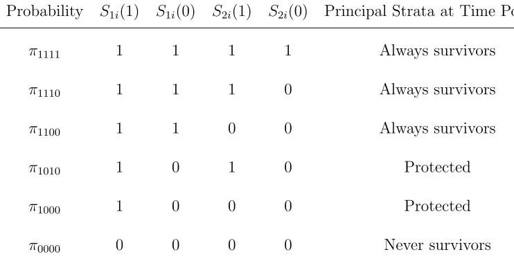
We further create finer strata based on the possible combinations of potential survival at both the first (QOL measurement point) and second (post-QOL mea-surement point) time points, which is described in Table 2.1.

(28)

Table 2.1: Fine Strata

Probability S1i(1) S1i(0) S2i(1) S2i(0) Principal Strata at Time Point 1 π1111 1 1 1 1 Always survivors

π1110 1 1 1 0 Always survivors

π1100 1 1 0 0 Always survivors

π1010 1 0 1 0 Protected

π1000 1 0 0 0 Protected

π0000 0 0 0 0 Never survivors

(29)

In terms of our fine strata, the SACE is expressed as:

SACE= E(Yi(1)−Yi(0)|S1i=S1i(0) = 1)

=P(Yi(1) = 1|S1i(1) =S1i(0) = 1)−P(Yi(0) = 1|S1i(1) =S1i(0) = 1)

= (π1111E(Yi(1)|1111) +π1110E(Yi(1)|1110) +π1100E(Yi(1)|1100))

π1111+π1110+π1100

−(π1111E(Yi(0)|1111) +π1110E(Yi(0)|1110) +π1100E(Yi(0)|1100))

π1111+π1110+π1100

(2.2.1)

Plausible assumptions can be made on data to tighten the bounds of SACE. Zhang and Rubin (2003) proposed the assumption that when assigned treatment, on aver-age, the outcome for “always survivors” is better than “protected”, in our case, that is to say P(Yi(1) = 1 |11) ≤ P(Yi(1) = 1| 10), recalling that we use 1 to denote

worse outcome for Y. This uses only the information on death before the measure-ment of the non-mortality outcome. In the rest of this chapter, we will refer to this assumption as the ranked average score with one stage survival information assump-tion. Survival information after measurement of the non-mortality outcome may deliver finer information, making use of which can help us make more reasonable as-sumptions and sharpen inferences. We will refer to the following set of asas-sumptions as ranked average score with two stage survival information assumptions.

Assumption 4. Among always survivors at time point 1, the probability of worse outcome for group 1111 is the lowest, whereas the probability of worse outcome for group 1100 is the highest under both treatment arms:

(30)

P(Yi(0) = 1|1111)≤P(Yi(0) = 1|1110)≤P(Yi(0) = 1|1100) (2.2.3)

Assumption 5. Among protected at time point 1, the probability of worse out-come for group 1010 is no higher than that for group 1000 under treatment:

P(Yi(1) = 1|1010)≤P(Yi(1) = 1 |1000) (2.2.4)

Assumption 6. Under treatment, the probability of worse outcome for group 1100 is not lower than that for group 1010, but not higher than that for group 1000, and the probability of worse outcome for group 1110 is not higher than that for group 1010:

P(Yi(1) = 1|1110)≤P(Yi(1) = 1|1010)≤P(Yi(1) = 1|1100)≤P(Yi(1) = 1|1000)

(2.2.5)

(31)

discharged home alive under treatment are healthier on average than patients who would ultimately die in the hospital. Assumptions 4 and 5 are plausible because being discharged home alive is a proxy for health at day 28. Assumption 6 is a comparison of the 1010 patients who would die before day 28 under control but survive to day 28 and be discharged home alive under treatment, to the 1100 patients who would survive to day 28 under both treatment and control but die in the hospital after day 28 under both treatment and control. Assumption 6 says that under the treatment, the 1010 patients tend to be healthier than the 1100 patients at day 28. This is plausible for the ARDSNet study for the following reasons. The 1100 patients are likely to be fairly sick by day 28 under the treatment since these patients will die in the ICU. In contrast, the 1010 patients are likely to be less sick on day 28 under the treatment because they will be (or already have) discharged home alive. An example of a 1010 patient would be a patient who was healthy but suffered a gunshot wound that caused an acute lung injury. When the patient arrives at the ICU, the patient is in critical condition and only the treatment will save the patient, but if the patient receives the treatment, the patient’s health before the gunshot wound will enable the patient to recover well and be regaining his or her health by day 28. In summary, assumptions 4, 5 and 6 are plausible for the ARDSNet study.

(32)

as-sumptions. The major difference is that the one-stage survival assumption assumes that always survivors, on average, have better QOL outcome than the protected, whereas our two-stage survival assumptions assume that one particular always sur-vivors group, 1100, has worse QOL outcome than a particular protected group, 1010, on average under treatment, which is a more reasonable assumption for the ARDSNet study. The differences in the bounds obtained under the ranked average score with one stage survival information assumption and our two stage survival information assumptions are presented in numerical examples and the analysis of ARDSNet study in section 2.3.3 and 2.7 respectively.

2.3 Derivations of Bounds

Under assumptions 1-6, the SACE is not point identified based on the knowledge of the observable joint distribution of (Di, S1i, S2i, Yi). However, we can use that joint

distribution to obtain an interval in which the SACE must lie. We first derive the bounds for the proportions in each stratum, then for fixed proportions we derive the bounds for the SACE. In this section, we assume that the joint distribution of (Di, S1i, S2i, Yi) is known; in section 2.6, we will discuss forming confidence intervals

(33)

2.3.1 Bounds for proportions of each stratum

Notice that the observable strata of (Di, S1i, S2i) are mixtures of fine strata (Table

1). Thus we can express the proportions of strata of (Di, S1i, S2i) by proportions

of fine strata. Combining this with the fact that all the proportions in the fine strata must lie between 0 and 1, we can obtain the bounds for each fine stratum’s proportion. We use ps1s2|d to denoteP(S1i = s1, S2i =s2 |Di =d). The following

equations hold:

p11|1 =π1111+π1110+π1010 (2.3.1)

p10|1=π1100+π1000 (2.3.2)

p00|1=π0000 (2.3.3)

p11|0=π1111 (2.3.4)

p10|0=π1110+π1100 (2.3.5)

p00|0 =π1010+π1000+π0000 (2.3.6)

Further we have,

0≤π1111, π1110, π1100, π1010, π1100, π1000, π0000 ≤1 (2.3.7)

Given (2.3.1)-(2.3.6), we can express eachπ by functions of pss|d andπ1100:

π1111=p11|0

(34)

π1010 =p11|1−p11|0−p10|0+π1100

π1000=p10|1−π1100

π0000=p00|1

and subject to the constraint of (2.3.7), we have,

max{0, p11|0+p10|0−p11|1} ≤π1100 ≤min{p10|0, p10|1} (2.3.8)

2.3.2 Bounds for the SACE

In this step, we first derive the bounds for the SACE with known proportions of each fine stratum, then will combine the result with the bounds obtained in section 2.3.1 to construct the final bounds for the SACE.

The observable strata of (Yi, S1i, S2i | Di) are mixtures of potential outcomes

from the fine strata. Letting qys1s1|d denote P(Yi = y, S1i = s1, S2i = s2 |Di = d),

we have the following identities:

(35)

Recall that

SACE = (π1111E(Yi(1)|1111) +π1110E(Yi(1)|1110) +π1100E(Yi(1)|1100))

π1111+π1110+π1100

−(π1111E(Yi(0)|1111) +π1110E(Yi(0)|1110) +π1100E(Yi(0)|1100))

π1111+π1110+π1100

(2.3.13) Given π0s, (π1111E(Yi(0)|1111)+π1110E(Yi(0)|1110)+π1100E(Yi(0)|1100))

π1111+π1110+π1100 =

q111|0+q110|0

π1111+π1110+π1100 which

is point identified. Thus to bound the SACE, we only need to boundπ1111E(Yi(1)|

1111) +π1110E(Yi(1)|1110) +π1100E(Yi(1)|1100), which defines a linear

program-ming problem:

min/max (π1111E(Yi(1)|1111) +π1110E(Yi(1)|1110) +π1100E(Yi(1)|1100))|π1100

(2.3.14) Subject to:

q₁₁₁_|₁=π1111E(Yi(1)|1111) +π1110E(Yi(1)|1110) +π1010E(Yi(1)|1010) (2.3.15)

q110|1 =π1100E(Yi(1)|1100) +π1000E(Yi(1)|1000) (2.3.16)

E(Yi(1)|1111)≤E(Yi(1)|1110)≤E(Yi(1)|1100) (2.3.17)

E(Yi(1)|1010)≤E(Yi(1)|1000) (2.3.18)

E(Yi(1)|1110)≤E(Yi(1)|1010)≤E(Yi(1)|1100)≤E(Yi(1)|1000) (2.3.19)

0≤E(Yi(1)|1111),E(Yi(1)|1110),E(Yi(1)|1100),E(Yi(1)|1010),E(Yi(1)|1000)≤1

(2.3.20)

(36)

The above linear programming problem has a solution if and only if q110|1 p10|1 ≥

q111|1

p11|1, which is an inequality that must be satisfied based on assumptions 4-6. For

each possible value ofπ1100, we solve the above linear programming problem; then,

combining this result with the bound forπ1100derived in section 2.3.1 thatπ1100∈I,

whereI = [max{0, p11|0+p10|0−p10|1}, min{p10|0, p10|1}], we have,

minSACE= min

π1100∈I[

min((π1111E(Yi(1)|1111) +π1110E(Yi(1)|1110) +π1100E(Yi(1)|1100))|π1100)−(q111|0+q110|0)

π1111+π1110+π1100

] =         

max{q111|1 +q110|1−p11|1−p10|1 +p11|0 +p10|0

p₁₁_|_{0 +}p₁₀_|₀ , q₁₁₁_|₁

p₁₁_|₁} −

q₁₁₁_|_{0 +}q₁₁₀_|₀

p₁₁_|_{0 +}p₁₀_|₀ , ifp11|0+p10|0−p11|1≥0

max{0,

q₁₁₁_|₁p₁₀_|_{1 +}q₁₁₀_|_{1 (}p₁₁_|_{0 +}p₁₀_|₀−p₁₁_|_{1 )} p₁₀_|_{1 (}p₁₁_|_{0 +}p₁₀_|_{0 )} } −

q₁₁₁_|_{0 +}q₁₁₀_|₀

p₁₁_|_{0 +}p₁₀_|₀ , ifp11|0+p10|0−p11|1<0 (2.3.21)

maxSACE= max

π1100∈I[

max((π1111E(Yi(1)|1111) +π1110E(Yi(1)|1110) +π1100E(Yi(1)|1100))|π1100)−(q111|0+q110|0)

π1111+π1110+π1100

]

=q111|1

p11|1

−q111|0+q110|0

p11|0+p10|0

+q110|1p11|1

−q111|1p10|1

p10|1p11|1(p11|0+p10|0)

·min{p10|0, p10|1} (2.3.22)

The details of the calculation for the bounds of SACE are provided in the Appendix.

2.3.3 Numerical Examples

Example 1

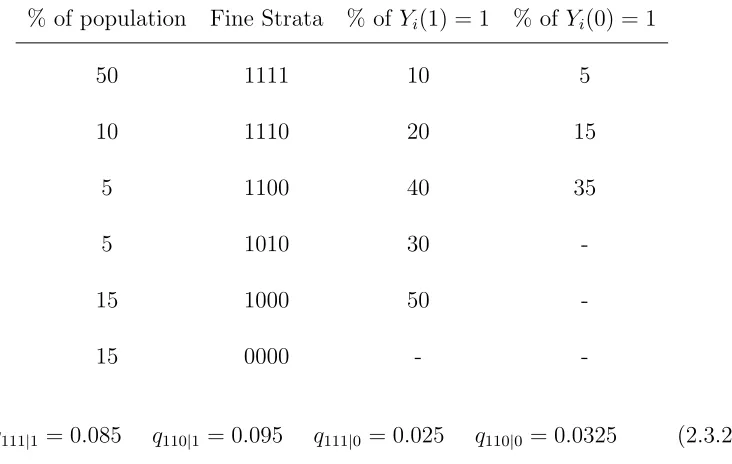
Assume that the underlying truth about the population is described by Table 2.2. The SACE = 0.05, meaning that the treatment will increase the probability of the worse non-mortality outcome by 0.05 among always survivors who will survive at least to the first time point under both treatment and control.

Suppose that we have an infinite sample, then we would observe that

p11|1 = 0.65 p10|1= 0.2 p00|1 = 0.15 p11|0= 0.5 p10|0 = 0.15 p00|0 = 0.35

(37)

Table 2.2: Setup 1

% of population Fine Strata % of Yi(1) = 1 % of Yi(0) = 1

50 1111 10 5

10 1110 20 15

5 1100 40 35

5 1010 30

-15 1000 50

-15 0000 -

-q111|1 = 0.085 q110|1 = 0.095 q111|0 = 0.025 q110|0 = 0.0325 (2.3.24)

Given the constraints imposed by the observed data (2.3.23)-(2.3.24) and assump-tions 4-6, we obtain the bound for SACE: [0.042, 0.122], showing that the treatment increases the probability of the worse non-mortality outcome.

However, if we don’t use the second time point survival information, the observed data would be:

P(S1i = 1|Di= 1) = 0.85 P(S1i= 1|Di = 0) = 0.65 (2.3.25) P(Yi = 1, S1i = 1|Di = 1) = 0.18 P(Yi = 1, S1i = 1|Di = 0) = 0.0575 (2.3.26)

(38)

Table 2.3: Setup 2

% of population Fine Strata % of Yi(1) = 1 % of Yi(0) = 1

50 1111 10 5

15 1110 20 15

5 1100 40 35

5 1010 30

-10 1000 50

-15 0000 -

-though the true SACE is positive. From this example, we see that making use of the survival information after measurement may provide us with more information and narrow the bounds on the SACE.

Example 2

(39)

The true SACE is 0.05. If we have an infinite sample, then we would have the following observed data:

p11|1= 0.7 p10|1= 0.15 p00|1 = 0.15 p11|0 = 0.5 p10|0 = 0.2 p00|0 = 0.3

(2.3.27)

q111|1 = 0.095 q110|1 = 0.07 q111|0 = 0.025 q110|0 = 0.04 (2.3.28)

Given the constraints imposed by the observed data (2.3.27)-(2.3.28) and as-sumptions 4-6, we obtain the bounds for the SACE: [0.043, 0.114]. If we don’t utilize the second time survival information, we would observe the following data:

P(S1i= 1|Di = 1) = 0.85 P(S1i = 1|Di = 0) = 0.7 (2.3.29) P(Yi = 1, S1i = 1|Di = 1) = 0.165 P(Yi = 1, S1i= 1|Di = 0) = 0.065 (2.3.30)

(40)

2.4 Extension to IV settings

The idea of using second time point survival information to sharpen the inference of SACE under randomized trials with perfect compliance can be naturally extended to randomized trials with noncompliance or observational studies with a valid IV to obtain inference about the complier survivor average causal effect (CSACE). In a randomized trial with noncompliance, the assignment of treatment can be used as an IV to assess the effects of receiving the treatment on the outcome. In ob-servational studies, natural experiments such as a person’s draft lottery number, randomly assigned federal judges or quarter of birth have been used as IVs. (An-grist, 1990; Angrist and Krueger, 1991; Kling, 1999). For more literatures on IV, see Angrist, Imbens, and Rubin (1996), Abadie (2002), Hernan and Robins (2006), Tan (2006), Brookhart and Schneeweiss (2007), Cheng (2009), and Clarke and Wind-meijer (2012).

Let Zi represent the binary IV; 1 encourages the treatment for the ith subject

and 0 does not provide encouragement of the treatment. We use Z to denote the vector of IV for all subjects. LetDi(z) be the potential binary treatment variable

that would be observed under IV assignment zfor subject i; 1 being the treatment and 0 denotes the control. LetS1i(z) be the potential survival indicator of subject

i that would be observed at the first time point after which the measurement of non-mortality outcome is taken; with 0 indicating death, 1 if alive. Let Yi(z)

(41)

IV assignment z. Again, the non-mortality outcome would be measured after the first time point, thus if the subject would die before that time point (S1i(z) = 0), Yi(z) is not defined; otherwise S1i(z) = 1 and Yi(z) = 1 or 0, 1 indicating a worse

outcome. We further define S2i(z) to be the potential indicator of survival at the

second time point for subject i that would be observed if under IV assignmentz. As in section 2.2, ifS1i(z) = 0, thenS2i(z) = 0 by definition. We useZi, Di, S1i, Yi and S2i to denote respectively the observed IV, treatment received, observed survival

indicator at the first time point, observed non-mortality outcome and observed survival indicator at the second time point for subject i.

2.4.1 Assumptions

We assume the following assumptions hold for the IV setup. These assumptions combine those of Angrist, Imbens and Rubin (1996) for the IV setup and the ranked average score with two stage survival information assumptions of section 2.2.

Assumption IV-1. Stable unit treatment value assumption (SUVTA).

• If zi = zi0, then Di(z) = Di(z0), S1i(z) = S1i(z0), S2i(z) = S2i(z0), and Yi(z) =Yi(z0)

SUVTA means that a subject’s potential treatments and outcomes are not affected by other individuals’ IV status and means that we can writeDi(z) asDi(zi), S1i(z)

(42)

Assumption IV-2. Nonzero average causal effect of Z on D. The average causal effect of Z on D, E[Di(1)−Di(0)], is not equal to zero.

Assumption IV-3. Independence of the instrument from unmeasured confounders: the random vector (D(1), D(0), S1(1), S1(0), S2(1), S2(0), Y(1), Y(0)) is independent

of Z.

Based on subjects’ compliance behavior, we can first partition the population into four groups:

Ui =

                            

00, if Di(1) =Di(0) = 0

10, if Di(1) = 1, Di(0) = 0

11, if Di(1) =Di(0) = 1

01, if Di(1) = 0, Di(0) = 1

(2.4.1)

where 00, 10, 11, and 01 represent never taker, complier, always taker and defier, respectively. Because Di(1) and Di(0) are never observed jointly, the compliance

behavior of a subject is unknown.

Assumption IV-4. Monotonicity of effect of IV on treatment: D(1) ≥ D(0). There is no U=01 group.

Assumption IV-5. Monotonicity of effect of IV on survival: S1i(1) ≥ S1i(0), S2i(1)≥S2i(0).

(43)

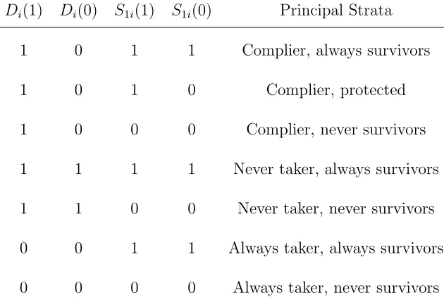
Table 2.4: Principal Strata

Di(1) Di(0) S1i(1) S1i(0) Principal Strata

1 0 1 1 Complier, always survivors 1 0 1 0 Complier, protected 1 0 0 0 Complier, never survivors 1 1 1 1 Never taker, always survivors 1 1 0 0 Never taker, never survivors 0 0 1 1 Always taker, always survivors 0 0 0 0 Always taker, never survivors

Assumption IV-6. Exclusion restrictions among never-takers and always-takers:

S1i(1) =S1i(0), S2i(1) =S2i(0), Yi(1) =Yi(0),for Ui= 00 or 11.

This means that the IV only affects the outcomes through treatment and has no direct effect on outcomes.

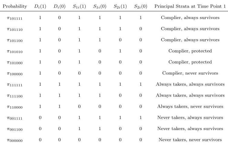
Based on the possible joint combinations of (Di(1), Di(0), S1i(1), S1i(0)) under

(44)

Table 2.5: Fine Strata

Probability Di(1) Di(0) S1i(1) S1i(0) S2i(1) S2i(0) Principal Strata at Time Point 1

π101111 1 0 1 1 1 1 Complier, always survivors

π101010 1 0 1 0 1 0 Complier, protected

π101000 1 0 1 0 0 0 Complier, protected

π100000 1 0 0 0 0 0 Complier, never survivors

π111111 1 1 1 1 1 1 Always takers, always survivors

π111100 1 1 1 1 0 0 Always takers, always survivors

π110000 1 1 0 0 0 0 Always takers, never survivors

π001111 0 0 1 1 1 1 Never takers, always survivors

π001100 0 0 1 1 0 0 Never takers, always survivors

π000000 0 0 0 0 0 0 Never takers, never survivors

control if IV is 0, and that would survive under both treatment such that the non-mortality outcome Y is well defined in both cases. Thus, it is the only group for which variation in the IV can identify the causal effect of the treatment on the non-mortality outcome: CSACE = E(Yi(1)−Yi(0)|1011).

(45)

In terms of the fine strata in Table 2.5, the CSACE is expressed as:

CSACE= E(Yi(1)−Yi(0)|1011)

=P(Yi(1) = 1|1011)−P(Yi(0) = 1|1011)

= (π101111E(Yi(1)|101111) +π101110E(Yi(1)|101110) +π101100E(Yi(1)|101100))

π101111+π101110+π101100

−(π101111E(Yi(0)|101111) +π101110E(Yi(0)|101110) +π101100E(Yi(0)|101100))

π101111+π101110+π101100

(2.4.2)

The same assumptions are made for compliers as we made for subjects under randomized trials with perfect compliance (Assumptions 4-6 in Section 2.2).

Assumption IV-7. Among ”complier, always survivors”, the probability of worse outcome for group 101111 is the lowest, whereas the probability of worse outcome for group 101100 is the highest under both treatment arms:

P(Yi(1) = 1|101111)≤P(Yi(1) = 1|101110)≤P(Yi(1) = 1|101100) (2.4.3) P(Yi(0) = 1|101111)≤P(Yi(0) = 1|101110)≤P(Yi(0) = 1|101100) (2.4.4)

Assumption IV-8. Among ”complier, protected”, the probability of worse out-come for group 101010 is no higher than that for group 101000 under treatment:

P(Yi(1) = 1|101010)≤P(Yi(1) = 1 |101000) (2.4.5)

(46)

that for group 101010:

P(Yi(1) = 1|101110)≤P(Yi(1) = 1|101010)≤P(Yi(1) = 1|101100)≤P(Yi(1) = 1|101000)

(2.4.6)

2.4.2 Derivations of Bounds

As for the SACE in randomized experiments setup, the CSACE is not point iden-tified without further assumptions based on the observable joint distribution of (Zi, Di, S1i, S2i, Yi), but can be bounded. We will again adopt the two step method

we used in section 2.3 to obtain the bound.

The observable strata of (Zi, Di, S1i, S2i) are mixtures of fine strata, if we use ps1s2d|z to denote P(S1i = s1, S2i = s2, Di = d | Zi = z), we have the following

identities:

p111|1 =π101111+π101110+π101010+π111111 (2.4.7)

p101|1 =π101100+π101000+π111100 (2.4.8)

p001|1 =π100000+π110000 (2.4.9)

p110|1=π001111 (2.4.10)

p100|1=π001100 (2.4.11)

p000|1=π000000 (2.4.12)

p110|0 =π101111+π001111 (2.4.13)

(47)

p000|0 =π100000+π000000+π101010+π101000 (2.4.15)

p111|0=π111111 (2.4.16)

p101|0=π111100 (2.4.17)

p001|0=π110000 (2.4.18)

and the constraint

0≤π101111, π101110, π101100, π101010, π101000, π100000, π111111, π111100, π110000, π001111, π001100, π000000≤1

(2.4.19)

Given (2.4.7)-(2.4.18), we can express each π in terms of ps1s2d|z andπ101100:

π000000=p000|1

π001111=p110|1

π001100=p100|1

π111111=p111|0

π110000=p001|0

π111100=p101|0

π100000 =p001|1−p001|0

π101111 =p110|0−p110|1

π101000 =p101|1−p101|0−π101100

π101110 =p100|0−p100|1−π101100

(48)

and subject to the constraint of (2.4.19), we have,

max{0, p110|0+p100|0+p111|0−p111|1−p110|1−p100|1} ≤π101100≤min{p101|1−p101|0, p100|0−p100|1}

(2.4.20)

Bounds for the CSACE

For fixed π0s, let qys1s2d|z denote P(Yi =y, S1i =s1, S2i =s2, Di = d|Zi =z). We

(2.4.21)

q1101|1=π101100E(Yi(1)|101100) +π101000E(Yi(1)|101000) +π111100E(Yi(1)|111100) (2.4.22)

q1110|1=π001111E(Yi(1)|001111) (2.4.23)

q1100|1=π001100E(Yi(1)|001100) (2.4.24)

q1111|0=π111111E(Yi(0)|111111) (2.4.25)

q1101|0=π111100E(Yi(0)|111100) (2.4.26)

q_1110|0=π101111E(Yi(0)|101111) +π001111E(Yi(0)|001111) (2.4.27)

q1100|0=π101110E(Yi(0)|101110) +π101100E(Yi(0)|101100) +π001100E(Yi(0)|001100) (2.4.28)

Recall that

CSACE= (π101111E(Yi(1)|101111) +π101110E(Yi(1)|101110) +π101100E(Yi(1)|101100))

π101111+π101110+π101100

−(π101111E(Yi(0)|101111) +π101110E(Yi(0)|101110) +π101100E(Yi(0)|101100))

π101111+π101110+π101100

(2.4.29)

Givenπ0s,

(π101111E(Yi(0)|101111)+π101110E(Yi(0)|101110)+π101100E(Yi(0)|101100))

π101111+π101110+π101100 =

q1110|0+q1100|0−q1110|1−q1100|1 π101111+π101110+π101100

which is point identified. Thus to bound the CSACE, we only need to bound

π101111E(Yi(1)|101111) +π101110E(Yi(1)|101110) +π101100E(Yi(1)|101100), which

defines a linear programming problem:

(49)

Subject to:

q1111|1−q1111|0=π101111E(Yi(1)|101111) +π101110E(Yi(1)|101110) +π101010E(Yi(1)|101010) (2.4.31)

q1101|1−q1101|0=π101100E(Yi(1)|101100) +π101000E(Yi(1)|101000) (2.4.32)

E(Yi(1)|101111)≤E(Yi(1)|101110)≤E(Yi(1)|101100) (2.4.33)

E(Yi(1)|101010)≤E(Yi(1)|101000) (2.4.34)

E(Yi(1)|101110)≤E(Yi(1)|101010)≤E(Yi(1)|101100)≤E(Yi(1)|101000) (2.4.35)

0≤E(Yi(1)|101111),E(Yi(1)|101110),E(Yi(1)|101100),E(Yi(1)|101010),E(Yi(1)|101000)≤1 (2.4.36)

where constraints (2.4.33)-(2.4.35) are imposed by assumptions (IV-7) - (IV-9). The above linear programming problem has a solution if and only if q1101|1−q1101|0

p101|1−p101|0 ≥

q1111|1−q1111|0 p111|1−p111|0 .

For each possible value of π101100, we can solve the above linear programming

problem; then, combining this result with the bound for π101100, let L = p110|0 +

p100|0+p111|0 −p111|1−p110|1−p100|1, U = min{p101|1−p101|0, p100|0−p100|1}, then

π101100 ∈I, where I = [max{0, L}, U], we obtain

maxCSACE=q1111|1

−q1111|0

p111|1−p111|0

−q1110|0−q1110|1+q1100|0−q1100|1

p110|0−p110|1+p100|0−p100|1

+(q1101|1

−q1101|0)(p111|1−p111|0)−(q1111|1−q1111|0)(p101|1−p101|0) (p101|1−p101|0)(p110|0−p110|1+p100|0−p100|1)(p111|1−p111|0)

·U

IfL≥0

minCSACE= max{q1111|1−q1111|0+q1101|1−q1101|0−p111|1+p111|0−p101|1+p101|0+p110|0−p110|1+p100|0−p100|1

p110|0−p110|1+p100|0−p100|1

,

q1111|1−q1111|0

p111|1−p111|0

} −q1110|0−q1110|1+q1100|0−q1100|1

p110|0−p110|1+p100|0−p100|1

IfL <0

minCSACE= max{(q1111|1−q1111|0)(p101|1−p101|0) + (q1101|1−q1101|0)(p110|0−p110|1+p100|0−p100|1−p111|1+p111|0)

(p101|1−p101|0)(p110|0−p110|1+p100|0−p100|1)

,

0} −q1110|0−q1110|1+q1100|0−q1100|1

(50)

2.5 Checking the plausibility of ranked average

score with two stage survival assumptions and

exclusion restriction assumptions

From the observable data, it cannot be determined whether our ranked average score with two stage survival information assumptions for randomized experiments setup or IV settings hold, also it cannot be determined whether the exclusion restriction assumed in the IV settings hold. However, there are some necessary conditions that the probability distribution of the observable data must satisfy when these assump-tions are valid. If these condiassump-tions are violated, then we know our assumpassump-tions do not hold.

For randomized experiments with perfect compliance, from the derivation of the bound for SACE in section 2.3, we know that the linear programming problem (2.3.14)-(2.3.20) under the ranked average score with two stage survival information assumptions as well as the constraints imposed by the observable”infinite sample” probability distribution has a solution if and only if

q110|1

p10|1

≥ q111|1

p11|1

(51)

the probability of the worse non-mortality outcome among the patients that are randomly assigned to treatment and that survive at least to the second time point. This is a direct result from our ranked average score with two stage survival as-sumptions (Asas-sumptions 4-6) which say that E(Yi(1) | 1111)≤ E(Yi(1)| 1110) ≤ E(Yi(1) |1010) ≤E(Yi(1) | 1100) ≤E(Yi(1) |1000). The first three expectations

are for subjects who can survive at least to the second time point under treatment and the last two expectations are for subjects who die before the second time point. For the IV setting of Section 2.4, based on the calculations in section 2.4.2, the corresponding necessary conditions that the probability distribution of the data must satisfy under Assumptions (IV-1)-(IV-9) are as follows: ,

q1101|1−q1101|0 ≥0, p101|1−p101|0 ≥0, q1111|1−q1111|0 ≥0, p111|1−p111|0 ≥0 (2.5.2)

q1101|1−q1101|0

p101|1−p101|0

≥ q1111|1−q1111|0

p111|1−p111|0

(2.5.3) Pearl (1995) provides a necessary condition on the joint probability distribution of the outcome, treatment and IV when the exclusion restriction holds. Extending Pearl’s result to our case where exclusion restrictions are assumed on both survival at the first time point and the second time point as well as a non-mortality outcome which may be censored, a necessary condition is that the following inequalities hold:

p00d|z1 +q010d|z2 +q110d|z3 +q011d|z4 +q111d|z5 ≤1 (2.5.4)

(52)

The above constraints to check the plausibility of our assumptions are for ”infi-nite sample” data. In practice, we can estimate the confidence with which the true observable population distribution satisfies the above constraints using a simple bootstrap procedure (Efron and Tibshirani, 1998). We bootstrap from the empirical distribution of the observed data and then count the percentage of the bootstrapped data sets for which the empirical distribution satisfies the constraints as an estimate of the confidence. Efron and Tibshirani (1998) provide some refinements on this simple bootstrap procedure that improve the accuracy of the estimated confidence.

2.6 Confidence Intervals for Bounds

In sections 2.3 and 2.4, the bounds we obtained are ”infinite sample” bounds where we assume that the joint distributions of (Di, S1i, S2i, Yi) or (Zi, Di, S1i, S2i, Yi) is

known. However, in practice, all these probabilities need to be estimated from the observed data. To account for the sampling uncertainty, we would like to construct confidence intervals for the bounds. The simplest way to construct confidence in-terval is through the Bonferroni method, where if we want an overall level of 1−α, we can obtain first the individual 1− α

2 confidence interval for the upper bound

(53)

confidence interval taking into account the joint distribution of the lower and up-per bound. The Horowitz and Manski confidence interval adds the same length to the upper and lower bounds in the confidence interval. Beran (1988) proposed the B method which also takes into account the joint distribution of upper and lower bounds without the restriction on the form of the confidence interval of the Horowitz and Manski confidence interval. A description of the above confidence in-terval approaches for bounds can be found in Cheng and Small (2006). Because of the nice properties of B method, we will use it to construct the confidence interval for the ARDSNet study.

(54)

good.

2.7 Application to ARDSNet Study

The ARDSNet study described in the introduction involved 861 patients with lung injury and acute respiratory distress syndrome who were randomized to receive mechanical ventilation with either lower tidal volumes or traditional tidal volumes. The non-mortality outcome variable we are interested in is whether patients were able to breathe without assistance by day 28 which is a measurement that reflects the quality of life for patients after treatment. We use Yi to represent this binary

quality of life measurement, with Yi being 1 indicating that the ith patient were

not able to breathe without assistance by day 28. Naturally, the first survival time point is day 28 after the treatment. If the patient died before day 28, then the non-mortality outcome could not be measured, thus will be undefined. The second time point survival indicator is whether the patient was eventually discharged home with unassisted breathing or not. We view the patients who received mechanical ventilation with lower tidal volume as the treatment group, and the patients who received mechanical ventilation with traditional tidal volume as the control group. LetDi equal 1 if theithpatient is randomized to treatment group, 0 if randomized

to control group. Further details on the data are described in appendix.

Table 2.6 presents the observed strata of (Di, S1i, S2i, Yi). Among the survivors

(55)

Table 2.6: Observed data for ARDSNet Study Number of Patients Di S1i S2i Yi

(56)

Table 2.7: The estimated bounds and 95% B method CIs of the SACE for ARDSNet study using ranked average score with two stage survival assumptions and one stage survival assumptions.

SACE Two-stage survival assumptions One-stage survival assumptions

Estimated bounds [−12.99%,−4.02%] [−17.38%,−4.27%]

95% confidence interval [−20.11%, 1.99%] [−27.57%, 2.18%]

without assistance by day 28 is 17.03% (which is 55/323); among the survivors in the traditional tidal volume group, the proportion of patients that cannot breathe without assistance by day 28 is 21.30% (which is 59/277). The difference of those two proportions−4.27% which is a direct comparison of the QOL among survivors in the lower tidal volume and survivors in the traditional tidal volume is likely an upward biased estimate for the SACE due to the informativeness of censoring by death.

The empirical distribution of (Di, S1i, S2i, Yi) satisfies the constraint (2.5.1).

Us-ing the bootstrap procedure, all of the 2000 bootstrapped datasets satisfy the con-straint (2.5.1), thus we are very confident that our set of two stage assumptions is plausible in the sense that it does not violate the constraint (2.5.1).

(57)

survive under both ventilation tidal volumes, the lower tidal volume would help re-duce the probability of breathing with assistance by day 28 by an amount between 4.02% to 12.99%. This bound for the SACE is substantially shorter, thus more informative, than the bound obtained through the one stage analysis which esti-mates the reduction to be between [4.27%,17.38%]. The 95% B method confidence intervals under both sets of assumptions cover 0, meaning that there is not strong evidence that ventilation with lower tidal benefits patients in terms of the quality of life outcome of breathing without assistance by day 28.

2.8 Conclusions and Discussions

(58)

We applied our method to the ARDSNet study. Making use of the post QOL measurement survival information (patients’ status when discharged home) in addi-tion to the pre-QOL survival informaaddi-tion (survival status at day 28) helps substan-tially shorten the bound on the SACE – the effect of lower tidal volume on being able to breathe without assistance by day 28.

(59)

bounds on the CSACE.

So far, we have assumed that we are in the context of a randomized trial or an observational study with a valid IV. Our method can also be naturally extended to the cases in which conditional on some discrete covariates there is ignorability such that the subjects are randomized or the IV is valid conditional on the covariates. We can stratify the subjects into subsets defined by each level of covariates, and apply our method to obtain the bound of SACE within each subgroup. Then we can obtain the overall bound of SACE combining the proportions of each subgroup. See (Freiman and Small, 2013) for more details on this topic. How to deal with the case in which the covariates are continuous requires further research.

(60)

Chapter 3 IV with Nonignorable Missing

Covariates

3.1 Introduction

3.1.1 Effect of type of delivery NICUs on premature infants

(61)

(62)

regionalization should probably not be a priority. Additionally, if only certain types of premature babies benefit from high level NICUs (e.g., only those below a certain gestational age), then resources would be best spent on increasing the rate of high level NICU delivery for those types of babies. To address this, we will estimate the effect of high level NICU delivery for babies with different characteristics, such as different gestational ages.

(63)

and a baby’s risk of mortality. To control for such unmeasured confounders, we will consider the instrumental variable (IV) method.

3.1.2 Instrumental variable approach

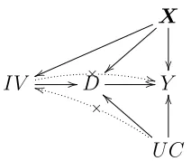
The IV method is widely used in observational studies (Angrist and Krueger, 1991; Baiocchi et al., 2010). An instrumental variable (IV) is a variable that is (i) as-sociated with the treatment, (ii) has no direct effect on the outcome, and (iii) is independent of unmeasured confounders conditional on measured confounders. The relationships between the IV, treatment(D), outcome(Y), measured confounders (X) and unmeasured confounders(U C) are shown in the directed acyclic graph in Figure 1. The basic idea of the IV method is to extract variation in the treatment that is free of the unmeasured confounders and use this confounder free variation to estimate the causal effect of the treatment on the outcome. The beauty of the IV method is that although treatment is not randomly assigned in observational stud-ies, the method still allows consistent estimation of the causal effect of a treatment.

X

}

v

IV //D× ++//Y

U C ×

k

k _a_a _O_O

(64)

The key assumptions for an IV are (i) the IV affects D; (ii) the IV does not have a direct effect on Y; (iii) the IV is independent of the unmeasured confounders UC given the measured confounders.

(65)

we are able to condition on are the month of pregnancy that prenatal care started (precare), mother’s education, and gestational age of the baby. We only have a small number of measured characteristics; for settings where there are a large numbers of measured characteristics, it is worth considering Lasso methods to control for the characteristics as in Imai and Ratkovic (2012). In previous work (Guo et al., 2014; Lorch et al., 2012), we used excess travel time as an IV to estimate the effect of high level vs. low level NICUs, but we did not account for the potential nonignorable missingness of certain measured characteristics. We will develop a method for accounting for nonignorable missing covariates.

3.1.3 Nonignorable missing covariates

(66)

(67)

at a high level NICU, she might be an always taker or complier.

Previous literature on IV with missing data has considered missing outcomes (Frangakis and Rubin, 1999; Levy, O’Malley and Normand, 2004; Mealli et al., 2004; Peng, Little and Raghunathan, 2004; Chen, Geng and Zhou, 2009; Small and Cheng, 2009). In this literature, it has been argued that ignorability of the missing outcome may only be plausible after conditioning on the covariatesand the partially observed compliance status (see (3.2.1)). Methods have been developed for estimating causal effects under this ”latent ignorability”. For missing covariates rather than missing outcomes, the only work on IV estimation that we are aware of is Peng, Little and Raghunathan (2004), which assumes missingness of covariates is ignorable conditional on observed data, but not allowed to depend on compliance behavior. In this chapter, we develop a method for estimation of the causal effect when the missingness of covariates may depend on the fully observed data as well as the partially observed compliance behavior.

(68)

EM algorithm to obtain the MLE estimates. We also provide a sensitivity analysis which allows for missingness to depend on further unobserved confounders besides compliance status.

(69)

rather than as part of a research study. For example, even if lab tests are always measured when a lab test is actually administered, since doctors will only order a lab test for some patients, there will be missing data. The missingness of lab values might be related to the treatment decision and outcome, and be nonignorable. For example, the decision to order a lab test is likely related to patient symptoms and/or disease severity, and we would expect that the probability of a lab test being ordered depends on what the value of the test would be, if measured, with unusual values being more likely to be measured (Roy and Hennessy, 2011). Thus, comparative effectiveness studies of drugs may need to consider instrumental variable methods with nonignorable missing covariates as in our study.

3.2 Notation and Assumptions

3.2.1 Notation

We use the potential outcome approach to define causal effects. Let Zi represent

the binary IV of infant i; 1 if excess travel time is less than 10 minutes, which encourages delivery in a high level NICU; 0 if excess travel time is more than 10 minutes, which does not provide encouragement of delivery in a high level NICU. In our data, 56.4% of subjects have excess travel time less than 10 minutes. We useZ to denote the vector of IVs for all infants. LetDi(z) be the potential binary

(70)

Di(z) be 1 if baby i would be delivered at a high level NICU under the vector of z

and 0 if the baby would be delivered at a low level NICU. We also letYi(z) denote

the potential binary outcome, neonatal death indicator, that would be observed for infant i under IV assignment z, with Yi(z) being 1 indicating that the newborn

would die in the hospital (neonatal death). We use Xi to denote the covariate

values for ith subject. The covariates in our study are discrete: infant’s gestational weeks, the month of pregnancy that prenatal care started and mother’s education, namely 8th grade or less, some high school, high school graduate, some college, college graduate, and more than college. For simplicity, we include the intercept in Xi. Finally, we let Rxi(z) be the binary response indicator of covariate x under

IV z, that is, Rx

i(z) = 1 if covariate x would be observed for infant i under IV

assignment z, and Rx_i(z) = 0 if covariate x would be missing. There is a Rx_i(z) for each covariate. In the above set of notations, Di(z), Yi(z) and Rxi(z) are all

potential outcomes of an infant. For each infant, depending on the value of z, one scenario is factual (observed), the other ones are counter factual (not observed). We useDi, Yi andRxi to denote observed treatment received, observed death outcome

of infant, and the observed response indicator for covariate x.

3.2.2 Assumptions

(71)

Assumption 1. Stable unit treatment value assumption (SUVTA) , meaning that a subject’s potential outcomes cannot be affected by other individuals’ status.

SUVTA allows us to write Di(z) as Di(zi), Yi(z) as Yi(zi) and Rxi(z)=R x i(zi).

This assumption is plausibly satisfied for our data since whether a mother delivers at a high level NICU and her baby’s outcome is unlikely to be affected by other mothers’ choice of living near to a high level NICU or not.

Based on subjects’ compliance behavior, we can partition the population into four groups:

Ui =

                            

n, ifDi(1) =Di(0) = 0 c, ifDi(1) = 1, Di(0) = 0 a, ifDi(1) =Di(0) = 1 d, ifDi(1) = 0, Di(0) = 1

(3.2.1)

where n, c, a, and d represent never taker, complier, always taker and defier, respec-tively. BecauseDi(1) andDi(0) are never observed jointly, the compliance behavior

of a subject is unknown. The parameter of interest in our study is the complier average causal effect (CACE), E(Yi(1)−Yi(0)|Ui=c,Xi =x).

Assumption 2. Nonzero average causal effect of Z on D. The average causal effect of Z on D, E[Di(1)−Di(0)], is not equal to zero.

(72)

low level NICU due to near NICUs being more convenient, thus assumption 2 is plausible.

Assumption 3. Independence of the instrument from unmeasured confounders: conditional onX, the random vector (Y(0), Y(1), D(0), D(1)) is independent of Z. This assumption is plausible for our study because premature delivery is unex-pected for women, so people do not choose where to live based on the closeness to high level NICU, especially after controlling for measured socioeconomic variable such as mother’s education level.

Assumption 4. Monotonicity: D(1)≥D(0).

If a mother is willing to travel to deliver at a high level NICU when living 10 or more minutes further to a high level NICU than a low level NICU, she is probably also willing to travel to deliver at a high level NICU when living less than 10 min-utes further to a high level NICU than a low level NICU.

Assumption 5. Exclusion restrictions among never-takers and always-takers:

Yi(1) =Yi(0) if Ui =n, and Yi(1) =Yi(0) if Ui =a.

(73)

time should not directly affect outcomes.

Assumption 6. Nonignorable missingness assumption (missingness ignorable conditional on compliance class, outcome and fully observed covariates): suppose the first k covariates ofX are fully observed, and the last m-k covariates have miss-ing values, then,

P(RXi,j

i (z)|Yi(z), Ui,Xi) =P(R Xi,j

i (z)|Yi(z), Ui, Xi,1, ..., Xi,k),∀j =k+ 1, ..., m.

This is saying that the missingness of covariates precare and mother’s education depends only on neonatal death information, compliance status of infant, gestational age (fully recorded) as well as the delivery level of NICU. It’s a plausible assumption for our data given the discussion in section 3.1.3.

Assumption 7. Exclusion restriction on missing indicator among never-takers and always-takers. RXi,j

i (1) =R Xi,j

i (0) if Ui =n, and R Xi,j

i (1) =R Xi,j

i (0) if Ui =a.

(74)

never takers should not be affected by the level of the IV.

3.3 Model and Estimation

We use a general location model (Olkin and Tate, 1961; Little and Rubin, 2002) for a mixture of continuous and categorical covariate variables, which could be easily adjusted for cases where covariates variables are all categorical or all continuous. We consider logistic models for (i) treatment assignment given covariates, (ii) out-come in each compliance class/ treatment assignment combination given covariates, and (iii) missingness in each compliance class/treatment assignment combination given covariates, and we use a multinomial logistic model for compliance class.

Model for covariate: Suppose that in the m covariates, the first p are categorical and the remaining m-p are continuous. We assign probability Wx1,...,xp to each

combination of possible values of those p categorical covariates variables, where

Wx1,...,xp are unknown parameters, and sum up to 1. • (Xi,1, ..., Xi,p) are iid distributed with

P((Xi,1, ..., Xi,p) = (x1, ..., xp)) =Wx1,...,xp, where

X

Wx1,...,xp = 1 (3.3.1) • Conditional on (Xi,1, ..., Xi,p) = (x1, ..., xp), we assume that the continuous

covariates random variables (Xi,p+1, ..., Xi,m) is multivariate normal with

un-known mean vector µ_x

(75)

and with unknown common positive definite covariance matrix Σ in order to reduce the number of parameters.

Xi,p+1, ..., Xi,m|(Xi,1, ..., Xi,p) = (x1, ..., xp)∼iidNm−p(µx1,...,xp,Σ) (3.3.2) Model for IV :

P(Zi = 1|Xi =x) =

exp (αTx)

1 + exp (αT_x₎ (3.3.3)

Model for compliance class :

P(Ui =n|Xi =x) =

1 1 + exp (δT

ax) + exp (δcTx)

(3.3.4)

P(Ui =c|Xi =x) =

exp (δT c x)

1 + exp (δT

ax) + exp (δTcx)

(3.3.5)

P(Ui =a|Xi =x) =

exp (δT ax)

1 + exp (δT

ax) + exp (δcTx)

(3.3.6)

Model for outcome :

P(Yi(z) = 1|Ui =u,Xi =x) =

exp (βT uzx)

1 + exp (βT uzx)

(3.3.7) According to assumption 4, βa0 = βa1,andβn0 = βn1. The quantity of interest is

the average treatment effect for compliers of each covariate level, which is estimated by E(Y(1)−Y(0)|U =c,X =x) = _{1+exp (}1_βT

c0x)

− 1

1+exp (βT

c1x)

.

Model for missingness indicators :

P(RXi,j_i (z) = 1|Yi(z) =y, Ui=u,Xi,1,...,k=x1,...,k) =

exp (θT

j,ux1,...,k+γj,uIy=1+ηj,uIz=1)

1 + exp (θT

j,ux1,...,k+γj,uIy=1+ηj,uIz=1)

(3.3.8)

(76)

Under the model (3.3.1)-(3.3.8), we seek to maximize the likelihood of the joint distribution of X, Z, U, Y, R. If we know the compliance classes and the missing covariates for each subject, we can get the MLE of parameters involved in those models easily. Based on this idea, we are going to use EM algorithm.

3.3.1 EM algorithm

For simplicity, we are going to present the EM algorithm for the case where all the covariates are categorical and that there are 4 covariates (including intercept) with only the first two completely observed, which is the case of our data. The EM algorithm can be easily extended to other scenarios. The first covariate is the intercept, and we further assume that the other three covariates are ordered categorical withq2, q3, q4 levels respectively. For a nominal categorical variable, we

can use indicator functions for each category, which the following algorithm could be easily adjusted for.

Let Nr3,r4,x2,x3,x4,u,z,y be the number of cases where R X3

i = r3, RXi 4 = r4, Xi,2 =

x2, Xi,3 = x3, Xi,4 = x4, Zi = z, Yi = y, Ui = u. Notice that Xi,1 = 1,∀i. Those

numbers are only partially observed, however, if they are known, the complete data log likelihood is,

lc =

X

r3,r4,x2,x3,x4,u,z,y

Nr3,r4,x2,x3,x4,u,z,y·(log(Wx2,x3,x4) + log(P(Zi=z|Xi= (1, x2, x3, x4)))

+ log(P(Ui=u|Xi= (1, x2, x3, x4))) + log(P(Yi=y|Zi=z, Ui=u, Xi= (1, x2, x3, x4)))

+ log(P(RXi,3

i =r3|Zi=z, Yi=y, Ui=u, Xi,2=x2))

+ log(P(RXi,4

(77)

Once we know N, the MLE estimates of the logistic models in (3.3.3)-(3.3.8) are standard, and the MLE for Wx2,x3,x4 ∝ N,,x2,x3,x4,,,, where N,,x2,x3,x4,,, is defined to

beP

r3,r4,u,z,yNr3,r4,x2,x3,x4,u,z,y.

In the E-step, conditional on observed data and parameters’ estimates obtained through the previous step, we can get the expected values for Nr3,r4,x2,x3,x4,u,z,y.

From the observed data, we can get the following counts:

1. N Nx2,x3,x4,d,z,y which denotes the number of cases that Xi,3, Xi,4 are both

observed and that Xi,2= x2, Xi,3=x3, Xi,4=x4, Di =d, Zi =z, Yi =y

2. N3x2,x4,d,z,y which denotes the number of cases that onlyXi,3 are unobserved

and that Xi,2 =x2, Xi,4 =x4, Di= d, Zi= z, Yi =y

3. N4x2,x3,d,z,y which denotes the number of cases that onlyXi,4 are unobserved

and that Xi,2 =x2, Xi,3 =x3, Di= d, Zi= z, Yi =y

4. N Bx2,d,z,y which denotes the number of cases thatXi,3, Xi,4 are both missing

and that Xi,2 =x2, Di= d, Zi =z, Yi =y

Further, letPr3,r4,x2,x3,x4,u,z,ybe the probability of a subject having case whereR X3 i = r3, RXi 4 = r4, Xi,2 = x2, Xi,3 = x3, Xi,4 = x4, Zi = z, Yi = y, Ui = u which are

calculated based on models (3.3.1)-(3.3.8). Then we can get the expected values for eachNr3,r4,x2,x3,x4,u,z,y, for example,

EN1,1,x2,x3,x4,a,1,y=N Nx2,x3,x4,1,1,y

P1,1,x2,x3,x4,a,1,y

(78)

To save space, all the formulas to update each Nr3,r4,x2,x3,x4,u,z,y are given in

appendix. By iteratively finding the E step estimate of N and maximizing the expected value of the complete data log likelihood in the M step until the algorithm converges, we obtain estimates of the parameters in models (3.3.1)-(3.3.8).

3.4 Simulation

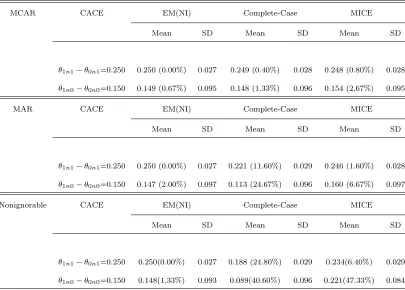
In this section, we conduct simulation studies to estimate the complier average causal effect in the simplest context where there is only one covariate, the values of which could only be 0,1. We consider the following three scenarios under assump-tions 1-7: 1) covariate is missing completely at random; 2) covariate is missing at random, meaning that the missingness does not depend upon the unobserved data, for example, does not depend on latent compliance status ; 3) missing mechanism for covariate is nonignorable: the missingness of covariate can depend on not only the observed outcome Y, treatment assignment Z, but also latent compliance status U.

(79)

with nonignorable missingness of covariates.

In the single covariate case, the models described in section 3 can be represented simply by the following set of parameters: Wu, which is P(Ui = u); Mu, which is P(Xi = 1 |Ui = u); ξx, which represents P(Zi = 1 |Xi = x); θzux, which denotes P(Yi(z) = 1 | Ui = u, Xi = x) and ρyzu, which are parameters for missingness

indicators P(Ri(z) = 1 | Yi = y, Ui = u), where Ri = 0 if covariate for ith subject

is missing. θ1c1−θ0c1 and θ1c0−θ0c0 are corresponding compliers’ average causal

effect for subjects with X being 1 and 0 respectively.

In all three scenarios, the parameters other than the ones in the missingness model are arbitrarily chosen and fixed as follows:

Wn = 0.2, Wa= 0.375, Mn = 0.5, Ma= 0.25, Mc = 0.8, ξ1 = 0.4, ξ0= 0.6

θ1n1 = 0.5, θ1n0= 0.3, θ0a1 = 0.8, θ0a0 = 0.7

θ1c1= 0.7, θ1c0 = 0.45, θ0c1 = 0.45, θ0c0 = 0.3

The missingness parameters in each scenario are described below, the values for

ρ0s are chosen to generate 12% missingness for covariate (the same missing rate as in the NICU study), and satisfy the exclusion restriction for missing indicator, which implies that ρy0a = ρy1a, andρy0n = ρy1n. In the first case, the missingness

(80)

affected by partially observed compliance status, so that the missingness won’t depend on unobserved data, which is a case of missing at random; in the last case, besides outcome and IV, the compliance status also plays a role in deciding the probability of missingness, and the values ofρ0_s_{are chosen so that even the largest}

effect of compliance status on missingness is still moderate (ρ11a−ρ11n = 0.25) and

realistic.

1. Missing Completely at Random

ρ11n =ρ01n =ρ10a=ρ00a=ρ11c =ρ01c =ρ00c =ρ10c = 0.88

2. Missing at Random

ρ11n =ρ10n =ρ10c = 0.88, ρ10a=ρ11a =ρ11c = 0.78 ρ01n =ρ00n =ρ00c = 0.94, ρ00a=ρ01a =ρ01c = 0.97

3. Nonignorable Missingness

ρ11n =ρ10n = 0.75, ρ01n =ρ00n = 0.8, ρ10a=ρ11a= 1 ρ00a =ρ01a= 0.95, ρ11c = 0.8, ρ01c = 0.9, ρ00c = 0.83, ρ10c= 0.97

Causal inference Methods for Addressing Censoring by Death and Unmeasured Confounding Using Instrumental Variables

University of Pennsylvania

ScholarlyCommons

Causal inference Methods for Addressing

Censoring by Death and Unmeasured

Confounding Using Instrumental Variables

Fan Yang

Causal inference Methods for Addressing Censoring by Death and

Unmeasured Confounding Using Instrumental Variables

Acknowledgments

Contents

Chapter 1

Introduction

Chapter 2

Two-stage Censoring by Death

2.1

Introduction

2.2

Notation and Assumptions: Randomized

Ex-periment with Perfect Compliance

2.2.1

Notation

2.2.2

Assumptions

2.3

Derivations of Bounds

2.3.1

Bounds for proportions of each stratum

2.3.2

Bounds for the SACE

2.3.3

Numerical Examples

2.4

Extension to IV settings

2.4.1

Assumptions

2.4.2

Derivations of Bounds

2.5

Checking the plausibility of ranked average

score with two stage survival assumptions and

exclusion restriction assumptions

2.6

Confidence Intervals for Bounds

2.7

Application to ARDSNet Study

2.8

Conclusions and Discussions

Chapter 3

IV with Nonignorable Missing

Covariates

3.1

Introduction

3.1.1

Effect of type of delivery NICUs on premature infants

3.1.2

Instrumental variable approach

3.1.3

Nonignorable missing covariates

3.2

Notation and Assumptions

3.2.1

Notation

3.2.2

Assumptions

3.3

Model and Estimation

3.3.1

EM algorithm

3.4

Simulation