e-ISSN: 2278-067X, p-ISSN: 2278-800X, www.ijerd.com
Volume 8, Issue 10 (October 2013), PP. 09-15
Design Methodology for Low Error Fixed Width Adaptive
Multiplier
Abida Yousuf
1, Roohie Naaz Mir
2, Hakim Najeeb-ud-din
31Ph.D Student, ECE Deptt, N.I.T, Srinager, India 2,3
Associate Professor, CSE Deptt, N.I.T, Srinager, India
Abstract:- In this paper, we develop a methodology for designing lower-error and Area efficient 2’s-complement fixed-width multiplier. In these multipliers basic multiplications follow the Baugh-Wooley algorithms and have been implemented using Field Programmable Gate Array (FPGA) devices. The approach is based on the fact that the multiplication operations used in multimedia applications (such as DSP) usually have the special fixed-width property i.e., their input data and output product have the same bit width. For some practical DSP applications, we only require n-bit multiplication output, which is to be obtained by directly truncating the n least-significant bits and preserving the n most significant bits. However, significant errors are introduced in the fixed-width operation, which are undesirable for DSP applications By properly choosing the generalized index and binary thresholding, we derive a better error-compensation bias to reduce the truncation error. The proposed fixed width low error multiplier shows better error performance as compared to other existing multiplier structures.
Keywords:-Bough Wooley Algorithm, Fixed Width Adaptive Multiplier, Multiplication., FPGA
I. INTRODUCTION
Multiplication is an important operation in many algorithms used in scientific computations such as Digital Signal Processing (DSP). The computational complexities of algorithms used in Digital Signal Processors (DSPs) have gradually increased over the years. Therefore, DSP’s require fast and efficient parallel multipliers for general purpose as well as application specific architectures. In these multipliers the basic multiplication follows the Baugh Wooley multiplier. The multipliers based on the Baugh–Wooley algorithm produce 2n-bit output with n-bit multiplier and n-bit multiplicand input. The DSP applications require extensive use of multiplication and squaring functions. A full width digital n × n multiplier computes the 2n output as a weighted sum of partial products. If the product is truncated to n-bits, the least-significant columns of the product matrix contribute little to the final result. To take advantage of this, truncated multipliers do not form all of the least-significant columns in the partial-product matrix. By eliminating more columns the area and power consumption of the arithmetic unit are significantly reduced and the delay also decreases. For some practical applications, we only require n-bit multiplication output, which is to be obtained by directly truncating the n least-significant bits and preserving the n most significant bits. However, significant errors are introduced in the fixed-width operation, which are undesirable for DSP applications [1].
To reduce the introduced truncation error, [2] proposed an analytical technique to generate a correction term. The main drawback of this design is the correction bias added to offset. The error due to truncation is a constant term and does not depend on the inputs being fed to the multiplier. [3] Proposed the fixed multiplier with a constant correction technique, which introduces a degree of flexibility in the number of columns that are truncated. This gives designers a chance to choose between area savings and better error correction. However, there exist two problems 1) how to choose proper indices. 2) Whether other lower error multipliers exist or not. The work in this paper proposes the general methodology for designing the lower error 2’s-complement fixed-width multiplier with w ≥ 1.
The rest of the paper is organized as follows: section 2 discusses the Baugh Wooley multiplier, section 3 gives details of the proposed algorithm, section 4 presents the results and section 5 provides the conclusion and references are listed in the end.
II.
BAUGH
WOOLEY
MULTIPLICATION
The Baugh wooley multiplication algorithm is an efficient way to handle the sign bits. This technique has been developed to design regular multipliers, suited for 2’s compliment mumbers.[1]
LET US CONSIDER Considering 2’s complement integer operands, a n-bit multiplicand X and a n-bit multiplier Y
2 1 1
0
2
2
n
n i
n i
i
X
x
x
(1)
2 1 1
0
2
2
n
n i
n i
i
Y
y
y
(2)Where
x y
i,
i
{0,1}
The standard product PStandard can be written as
=
2 2 2 2
2 2 1 1 1 1
1 1 1 1
0 0 0 0
2 2 2 2 2 1 2 2 2 1
n n n n
n ij n n j n n j
n n i j n i n j
i j i j
x y x y x y y x
(3)
(A) Fixed Width Multiplication
The multiplication based on the Baugh wooley algorithm produce 2n bit output with n bit multiplier and n bit multiplicand input. However in DSP applications only n bit multiplication output is needed. Therefore the fixed width multiplier is obtained by truncating the least significant partial products. And preserving the most significant partial products as shown in figure 1.
Fig.1: Partial product array diagram for an n × n Baugh-Wooley multiplier.
The most accurate fixed width product is theoretically given as
2
tan
n
P
MP
S
dard
temp
Where
2
nLP
temp
(4)
tan 1 0 0 1 2 2 0 0 2 1 1 0 0 1 0 0
1 1 1 1
... ... ...
2 2 2 2
S dard n n n n n n
P x y x y x y x y x y x y x y
(5)
Where temp an ideal error-compensation term called true rounding approach and it is infeasible to
it is observed that temp is mainly affected by
1 0 2 1 0 1
1
... 2 xny xny x yn
due to the largest weight. Now, let us
assume the main error compensation term Emain and remaining error compensation term Eremain [2, 3].
Therefore,
1
1 0 2 1...
0 1
2
main n n n
E
x
y
x
y
x y
(6)And
1
1
2 0...
0 2
...
1
2
1 0...
0 1
1
1
0 02
2
2
remain n n n n
E
x
y
x y
x y
x y
x y
(7) The equation (2) can be rewritten as
1
2
E
mainE
remaintemp
(8)Note that temp varies as the input bits xi’s or yi’s alternates.
Next we first define a generalized index, index,w, where w means to keep n+w most significant columns of the
sub-product array as shown in Figure 1 [4], and the binary parameters
q
n 1 w,
q
n 2 w,...,
q
0
0,1
.,
1,
2,...,
0
1 0
1
2 0
2...
0 1
0n w n w w
n w n w
q q q
index w
q
n wq
n wq
x
y
x
y
x y
n w
(9) The operator
i
q
i j i j
x y
x y
if qi=0
x y
i j if qi=1(10)
To introduce the generalized index into the error compensation bias equation we rewrite equation 8 as
,
1
,2
Q w
E
mainE
remain Q wtemp
(11) where index
12
n 1 w 22
n 2 w...
02
0
n w n w
Q
q
q
q
Where Q has a range varying from 0 to 2n-1+1.
III.
PROPOSED
FIXED
WIDTH
MULTIPLIERS
WITH
W
1
The lower truncation error can be obtained if larger most significant columns are kept in hardware, however at the cost of area. Equation (8) can be rewritten as
2 1
2 1
...
1 22
n w
q q
temp n w n w w
K
x
y
x y
(12) Where
1 0
1 0 0 1 ,
1
1
2
2
n w
q q
n w n w main remain Q w
K
x
y
x y
E
E
(13)In equation (12), the first term in the bracket is referred to as coarse-adjustment term and the second term [K] is referred to as fine-adjustment term. The coarse adjustment term can be easily realized by a simple circuit using AND, OR logic, while the index is decided. On the other hand, the value of the fine-adjustment term can be obtained by the expected value in rounding operation after analyzing the statistics [5].
Type 1
, 1 2 1 2
...
1 2 1
12
n
q q
tempQ w n n w
K
x
y
x y
if Q,w=02 1 2
...
1 2 1
22
n
q q
n n w
K
x
y
x y
if Q,w>0 (14)Type 2
, 1 2 1 2
...
1 2 1
32
n w
q q
tempQ w n w n w
K
x
y
x y
if Q,w>n2 1 2
...
1 2 1
42
n w
q q
n w n w
K
x
y
x y
if Q,w=n (15)Where K1, K2, K3, K4 are average values of K for satisfying index = 0, index >0, index >n, index = n respectively.
The restriction on the value of K can be limited as
K
i
0,1, 2
w 11, 2
w1
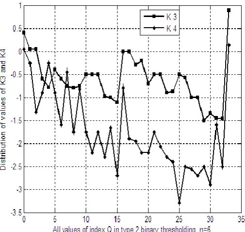
for i = 1, 2, 3 and 4.[6, 7]. By doing simulations we obtained the values K at different generalized indexes as shown in figure 2. we simulate the value of K for smaller word length while for large word lengths the value of K is determined by statistical analysis because at large word lengths we are not able to simulate the value of K due to high computational load.Fig. 2: Values of K versus different values Q of the Binary thresholding for n=6
(A )Statistical Analysis:
For bias estimation , we assume Type 2 binary thresholding,, which is defined in equation (15). After analyzing equation (15), two cases can be taken into consideration.
CASE 1
1
2n 1
n
1
1 3
3
1
1
2
2
main2 4
4
4
8
2
n
E
E
n
Where
1
4
i j
E x y
and
3
4
i j
E x y
Further
2 3
1
1
1
1
1
1
1
2
...
1
2
remain4 2
2
2
n8
4
n
E
E
n
n
The generalized index is
1 2 1 2 1
2 1
1
, 1
n n n i j main Q
i j n i j n
x
y
x
y
x y
E
K
3
E K
2 1 1 2
1
1
2
2
n n main remain
E x
y
x y
E
E
3
3
1
1
1
4
4
8
2
8
4
n
n
(16)CASE 2
1
2n 1
n
This condition is met when
2 1 1 2
1
n n
x
y
x y
and
x
n2y
1
...
x y
1 n2
1
Also
2 3 1
1
1
1
1
1
1
1
1
1
1 2
3
1 2
4
..
1 2
1 1
2
remain2
3
2
3
2
n3
2
n9
E
E
n
n
1
5
2
n
3
if n 4Therefore,
4
2 1 1 21
1
0
2
2
n n main remain
K
E K
E x
y
x y
E
E
(17)Thus from equations (16), (17) and (15), we can derive a new error compensation bias as.
2 1
, 1 2 1 1 2
1
...
2
n w
q q
tempQ w
x
n wy
x y
n w w
if
2n11
n
2 1 n w2
...
1 2 10
q q
n w n w
x
y
x y
if
2n11
n
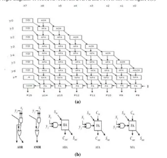
(18)Therefore, this constant approximation for can be mapped to the structure as shown in figure 3(a) for n=8 [8], where A, ND, HA, and FA denote AND gate, NAND gate, a half adder and a full adder, respectively. The logic diagrams of AOR, ANOR, AHA, AFA, and NFA is shown in figure 3(b)
(a)
(b)
Fig.3: (a) Proposed low-error fixed-width 8 x 8 Baugh Wooley multiplier with
Q2n11,w1, and (b) LogicalElements.
IV. RESULTS
The figure 4 shows the comparison between Booth and Baugh Wooley multiplication technique in terms of delay and we conclude that Baugh Wooley algorithm is the efficient one. The table1 shows the error performance of different fixed width multipliers. The Table 2 gives the comparison of standard and fixed width multiplier in terms of number of occupied slices and delay.
Table 1: Comparison results of error among different fixed width Baugh Wooley multipliers.
Table 2: Comparison results of Area and delay among different Baugh Wooley multipliers n=8
IV.
CONCLUSIONS
By properly choosing the generalized index and binary thresholding, we derive a better error-compensation bias to reduce the truncation error and then construct a lower error fixed-width multiplier, which is area-efficient for VLSI realization. Moreover, a number of low error fixed width multipliers are generated, the only constraint is to choose the right value of the index which would need exhaustive search.
REFERENCES
[1]. C. R. Baugh and B. A. Wooley, “A two’s complement parallel array multiplication algorithm,”
IEEE Transaction on Computers, vol. C-22, no. 12, pp.1045-1047, December 1973.
[2]. S. S. Kidambi, F. El-Guibaly, and A. Antoniou, “Area efficient multiplier for digital signal processing applications,” IEEE Transaction on Circuit, Systems II, vol. 43, pp. 90-94, 1996.
[3]. E. E. Swartzlander, Jr, “Truncated multiplication with approximate rounding,” Proceedings 33rd Conference on Signals, Systems, and Computer, vol. 2, pp. 1480- 1483, 1999.
[4]. Tu and Van, “Power efficient pipelined reconfigurable fixed width Baugh Wooley multiplier,” IEEE Transaction on Computers, vol. 58, no. 10, October, 2009.
[5]. Min-An Song, Lan-Da Van, Ting-Chun Huang, and Sy-Yen Kuo, “A Generalized Methodology for Low-Error Fixed-Width Booth Multipliers,” IEEE 47th Symposium on Circuits and Systems, July, 2004.
[6]. Jer Min Joa, Shiann Rong Kuang, and Ren Der Chen, “Design of low error fixed width multipliers for DSP applications,” IEEE Transaction on Circuits and Systems-II: vol. 46, no. 6, June, 1999.
[7]. Lan – Da –Van , and Chih - Chyau Yang , “ Generalized Low – Error Area- Efficient Fixed - Width Multipliers,” IEEE Trans On Circuits And Systems, vol.52, no. 8, August, 2005.
[8]. Muhammad H. Rais, B.M. Al-Harthi, Saad I. Al-Askar and F. K. Al. Hussein, “Design and Implementation of Basic Building Blocks of Power-Efficient Baugh Wooley Multipliers,” American Journal. Engineering and Applied Science, pp. 307-311, 2010.
[9]. Nicola Petra, Davide De Caro, Valeria Garofalo, Ettore Napoli, and Antonio G. M. Strollo,“ Truncated Binary Multipliers With Variable Correction and Minimum Mean Square Error.” ,” IEEE Transaction on Circuits and Systems-II: vol. 57, no. 6, June, 2010.
[10]. Y. C. Liao, H. C. Chang, and C. W. Liu, “Carry estimation for two’s complement fixed-width multipliers,” in Workshop on Signal Process. Syst. (SiPS), Oct. 2006, pp. 345–350.
Multiplier
Width Max Error
Mean Square Error
Fixed width multiplier w = 0
N = 8 -0.1156 3.3061 x 10⁻⁵
Fixed width multiplier w = 1
N = 8 -0.0078 8.2652 x 10⁻⁶
Multiplier No. of occupied LUT slices
Delay(ns) No. of IOB
Standard 86 10.878 32