A Study on Modal Parameter Estimation Method based on Operational Modal Analysis for Ship Structure



Abstract— A mathematical formulation of data-driven stochastic subspace identification (SSI) has been summarized and a code has been implemented for the modal parameter estimation of the ship structure. The implemented code has been verified and validated through the benchmark test of a rectangular plate, where the results have been compared with those of the commercial software. Then the code has been used to estimate the modal parameters of an oil tanker. The results show that the code operates well its function and provides stable solution by appropriately selecting key parameters related to the stability of the solution in data-driven SSI.

Index Term— Modal Parameter Estimation; Vibration Measurement; System Identification; Stochastic Process; Ship Vibrations

I. INTRODUCTION

THE modal parameter such as modal frequency, modal damping and modal shape is a key factor characterizing the dynamic behavior of structures, which could be estimated often using a dynamic model deterministically constructed based on physical information and fundamental law of motion of the target structures. When the physical information of the target structure is given, the dynamic model could be implemented via numerical scheme like finite element analysis. Besides, when limited, it should be via experimental method like experimental modal analysis (EMA) [1]. EMA is a traditional technique to extract the modal parameter of the structure, and uses frequency response functions which can be obtained when both of the excitation force as input and the response as output are known. Because, however, measuring the excitation force is impracticable in many engineering applications, especially for a large built-up structure like a ship structure, an alternative way like operational modal analysis (OMA) technique is adopted. OMA unlike EMA requires only responses not excitation forces. Accordingly, it is called output only modal analysis technique. Thus OMA can evaluate the modal parameter of the object structure by processing the response data easily measured during normal operation condition, consisting of various effects by boundary condition,

machineries’ coupling forces, wind forces, and hydro-dynamic forces. Owing to this advantage, OMA is suitable for modal parameter extraction of the large ship structure.

During few decades, OMA has been implemented to various methods [2]: peak picking method (PP) [3], frequency domain decomposition method (FDD) [4], auto regressive moving averages models (ARMA) [5], stochastic subspace identification method (SSI) [6], etc. PP extracts the modal parameter from each peak identified from the averaged power spectral densities at all measurement points. FDD extracts by carrying out singular value decomposition of the response spectra in frequency domain. ARMA uses an idealized mathematical model for response time data or their correlation functions evaluated using fast Fourier transform algorithm. SSI, a linear system identification method, has been implemented to data-driven SSI using response time series and covariance-driven SSI using their response correlation functions.

Data-driven SSI first proposed by Van Overschee and De Moore [7] identifies the state space matrices characterizing the dynamic behavior of the structure, which is based on numerical techniques such as QR-factorization for data reduction and singular value decomposition for noise rejection. This has been successfully applied to various types of large structures: wind turbine [6], ship [8], bridge [9], etc.

In this study, a mathematical formulation of data-driven SSI is summarized and a code is implemented to estimate the modal parameter of the ship structure. In order to verify and validate the implemented code, a benchmark test of the modal parameter estimation is carried out of a rectangular plate. The results are compared with those of the commercial software and the effect of key parameters related to the stability of the solution in data-driven SSI is investigated. Finally, the implemented code is applied for the modal parameter estimation of the real ship structure.

II. MATHEMATICAL FORMULATION AND IMPLEMENTATION

A. Dynamic model

The dynamic behaviour of the structure with n-degree of freedom is explained often with the following dynamic motion equation.

A Study on Modal Parameter Estimation Method

based on Operational Modal Analysis for Ship

Structure

Kookhyun Kim

School of Naval Architecture & Ocean Engineering, Tonmyong University 428, Sinseon-ro, Nam-gu, Busan, 48520, Republic of Korea

𝑀𝑢̈(𝑡) + 𝐷𝑢̇(𝑡) + 𝐾𝑢(𝑡) = 𝑓(𝑡) (1)

where 𝑀 ∈ 𝑅𝑛×𝑛, 𝐷 ∈ 𝑅𝑛×𝑛 and 𝐾 ∈ 𝑅𝑛×𝑛 are the mass, damping and stiffness matrices, respectively. f(t) ∈ Rn is the force, and 𝑢(𝑡) ∈ 𝑅𝑛 is the system response (displacement). (∙)̇ is the derivative operator with respect to the time 𝑡.

By introducing the state-space model, the equation (1) yields the following continuous-time stochastic state-space equation. 𝑥̇(𝑡) = 𝐴𝑐𝑥(𝑡) + 𝐵𝑐𝑓(𝑡) (2)

where 𝑥(𝑡) = [𝑢(𝑡)_{𝑢̇(𝑡)] ∈ 𝑅}2𝑛 is the continuous-time state space. 𝐴𝑐= [ 0_𝑀−1_{𝐾 −𝑀}𝐼−1_𝐷] ∈ 𝑅2𝑛×2𝑛 is the continuous-time system matrix characterizing the dynamic behavior of the structure. 𝐵𝑐= [ 0

𝑀−1] ∈ 𝑅2𝑛×𝑛.

The equation (2) is a first-order ordinary differential equation (ODE) and is easier to implement using a simple recursive algorithm than the equation (1) of the second-order ODE. Despite this advantage, it is sometimes impractical due to the fact that the response data sets of all degree of freedom should be required. Accordingly, transforming the original space 𝑥(𝑡) to the observation space 𝑦(𝑡) ∈ 𝑅𝑙 by the equation (3) is useful when the response data sets all degrees of freedom are not available from measurements.

𝑦(𝑡) = 𝐶𝑐𝑥(𝑡) + 𝐷𝑐𝑓(𝑡) (3)

where 𝐶_𝑐∈ 𝑅𝑙×2𝑛 is a system matrix describing a geometrical transformation from the original space to the observation space. 𝐷𝑐∈ 𝑅𝑙×𝑛_{. 𝑙 is the number of available response data sets.}

By discretizing the equation (3) in time, the discrete-time state space model is obtained below.

𝑥𝑘+1= 𝐴𝑥𝑘+ 𝐵𝑓𝑘

𝑦𝑘= 𝐶𝑥𝑘+ 𝐷𝑓𝑘 (4)

where 𝑥𝑘 = 𝑥(𝑘∆𝑡), 𝑦𝑘= 𝑦(𝑘∆𝑡), 𝑓𝑘= 𝑓(𝑘∆𝑡), 𝐴 = 𝑒𝐴𝑐∆𝑡, 𝐵 = (𝐴 − 𝐼)𝐴𝑐−1_𝐵

𝑐.𝑘 is the discrete-time sampling index of data. ∆𝑡 is the discrete-time sampling interval.

Considering unmeasurable system noise simplifies the equation (4) to the following.

𝑥𝑘+1= 𝐴𝑥𝑘+ 𝑤𝑘

𝑦𝑘 = 𝐶𝑥𝑘+ 𝑣𝑘 (5)

where 𝑤𝑘(= 𝐵𝑓𝑘) is the process noise of disturbances in system and inputs, and 𝑣_𝑘(= 𝐷𝑓_𝑘+ 𝑛_𝑦,𝑘 , 𝑛_𝑦,𝑘: the output noise) is the measuring noise.

One knows that the discrete-time system matrices 𝐴 and 𝐶 in the equation (5) contain the information of the dynamic characteristic and geometrical transformation of the structure. Accordingly, it could be used later to estimate the modal parameter of the structure by performing an eigen-value decomposition of the matrices.

B. Dada-driven SSI

The responses, which might be displacement, velocity and acceleration measured from the structure, are assembled with the data set matrix 𝑌 ∈ 𝑅𝑙×𝑁 below.

𝑌 = [𝑦1 𝑦2 ⋯ 𝑦𝑁] (6)

where 𝑁 is the discrete-time sampling number of the response data.

Meanwhile, a block Hankel matrix is built-up from the data set matrix 𝑌 as follows.

𝐻 = 1 √𝑁−2𝑠

[

𝑌(:,1:𝑁−2𝑠) 𝑌(:,2:𝑁−2𝑠+1)

⋮ 𝑌(:,2𝑠:𝑁) ]

= [𝐻𝑝 𝐻_𝑓] ∈ 𝑅

2𝑠𝑙×(𝑁−2𝑠) ₍₇₎

where 𝐻𝑝= 𝐻(1:𝑠,:)∈ 𝑅𝑠𝑙×(𝑁−2𝑠) and 𝐻𝑓 = 𝐻(𝑠+1:2𝑠,:)∈ 𝑅𝑠𝑙×(𝑁−2𝑠) _{are called the past and future matrices, respectively,} in the data-driven SSI technique. 𝑠is the number of data block. The block Hankel matrix is too large in size to handle so that a data-order reduction technique like an orthogonal projection should be applied. When dealing with large-size stochastic data like this, the projection can be often defined as a conditional mean of the future Hankel matrix with respect to the past one. Assuming the Gaussian process, projecting the future to the past 𝑂 is implemented by combining the covariance of the related matrices [7];

𝑂 = 𝐸(𝐻𝑓|𝐻𝑝) = 𝐻𝑓𝐻𝑝𝑇_{(𝐻𝑝𝐻𝑝}𝑇₎−1_{𝐻𝑝∈ 𝑅}𝑠𝑙×(𝑁−2𝑠) ₍₈₎

In theory, the equation (8) can be directly calculated, but in practice, adopting the data-order reduced matrix of the block Hankel matrix is preferable. Thus, the projection of the future row space to the past row space is defined as

𝑂 = 𝐿21𝑄1𝑇 ₍₉₎

where 𝐿21∈ 𝑅𝑠𝑙×𝑠𝑙 and 𝑄1𝑇 ∈ 𝑅𝑠𝑙×(𝑁−2𝑠) are obtained by the

LQ decomposition of the block Hankel matrix below.

𝐻 = [𝐿11 0 𝐿21 𝐿22] [𝑄1

𝑇

𝑄2𝑇]

(10)

where 𝐿11, 𝐿21, 𝐿22∈ 𝑅𝑠𝑙×𝑠𝑙. 𝑄1𝑇, 𝑄2𝑇 ∈ 𝑅𝑠𝑙×(𝑁−2𝑠). (∙)𝑇 is the transpose operator.

Additionally, the projection matrix of the equation (10) is factorized to the observability matrix 𝛤 ∈ 𝑅𝑠𝑙×𝑚 and the Kalman filter state 𝑋 ∈ 𝑅𝑚×(𝑁−2𝑠).

𝑂 = 𝛤𝑋 (11)

where m is the system order which is the specified by user and determines the accuracy of the solution.

decomposition technique (SVD) of the weighted projection matrix 𝑊𝑂𝐼 is performed as follows.

𝑊𝑂𝐼 = 𝑈𝑆𝑉𝑇 _{= [𝑈1 𝑈2] [}𝑆1 0 0 𝑆2≈ 0] [𝑉1

𝑇

𝑉2𝑇]

≈ 𝑈1𝑆1𝑉1𝑇 ∈ 𝑅𝑠𝑙×(𝑁−2𝑠) (12)

where 𝑊 = (𝐻𝑓𝐻𝑓𝑇)− 1

2∈ 𝑅𝑠𝑙×𝑠𝑙 is the pre-multiplied weighting matrix. The identity matrix 𝐼 ∈ 𝑅(𝑁−2𝑠)×(𝑁−2𝑠) is the post-multiplied weighting matrix. 𝑈₁∈ 𝑅𝑠𝑙×𝑚, 𝑆₁∈ 𝑅𝑚×𝑚 , 𝑉1𝑇 ∈ 𝑅𝑚×(𝑁−2𝑠).

Then, the observability matrix is calculated by the following equation.

𝛤 = 𝑊−1_𝑈 1𝑆1

1

2_{∈ 𝑅}𝑠𝑙×𝑚 ₍₁₃₎

Finally, the system matrix 𝐴 and 𝐶 are estimated from the observability matrix by the equations (14) and (15).

𝐴 = 𝛤(𝑙+1:𝑠𝑙,:)+ 𝛤(1:(𝑠−1)𝑙,:)∈ 𝑅𝑚×𝑚 (14)

𝐶 = 𝛤(1:𝑙,:)∈ 𝑅𝑙×𝑚 (15)

where (∙)+is the pseudo inversion operator.

C. Modal parameter calculation

The matrix 𝐴 is eigen-value decomposed.

𝐴 = 𝛹𝛬𝛹−1_{∈ 𝑅}𝑚×𝑚 ₍₁₆₎

where 𝛹 ∈ 𝑅𝑚×𝑙and 𝛬 = [

𝜆1 0 0 0 0 𝜆2 0 0 0

0 00 ⋱ 0 0 𝜆𝑚

] ∈ 𝑅𝑚×𝑚 _{are the}

eigen-matrix and the diagonal eigen-value matrix in the state space, respectively. 𝜆_𝑖𝑖-th eigen value of the system.

These matrices and the transformation matrix 𝐶 are used to calculate modal parameter in the physical space with the following equations.

𝑓𝑖=|𝑙𝑛(𝜆_{2𝜋𝛥𝑡}𝑖)| (17)

𝜂𝑖= −𝑅𝑒[𝑙𝑛(𝜆𝑖)]

|𝑙𝑛(𝜆_𝑖)| (18)

𝛷 = 𝐶𝛹 ∈ 𝑅𝑙×𝑚 ₍₁₉₎

where 𝑓_𝑖 and 𝜂𝑖 are the modal frequency and the modal damping of 𝑖-th mode of the system, respectively. 𝑅𝑒[∙] is the real part of the complex value. 𝛷 = [𝜑1 𝜑2 ⋯ 𝜑𝑀] ∈ 𝑅𝑙×𝑚 _{is the modal matrix consisting of mode shape vectors} 𝜑𝑖∈ 𝑅𝑙_.

D. Implementation

A code has been implemented using MATLAB based on the data-driven SSI. The code operates in the procedure presented in Fig. 1, which consists of assembling data set matrix, build-up block Hankel matrix, orthogonal projection, observability matrix calculation, system matrix estimation, modal parameter calculation, etc.

III. BENCHMARK TEST

A. Benchmark test

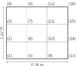
The implemented code is validated and verified through a benchmark test of a rectangular plate which is provided as an example in the commercial software ARTeMIS [10]. The width and length of the rectangular plate are 0.26m and 0.22m, respectively. A data set for assembling data set matrix 𝑌 has been obtained also from an example file in ARTeMIS, which consists of time-series acceleration data sets gathered from 16 uniform grid points designated in Fig. 2. The data sampling frequency and the data length are 4,096 Hz and 60 seconds, respectively. No information except for the above are provided.

Fig. 1. Modal parameter estimation procedure implemented in MATLAB

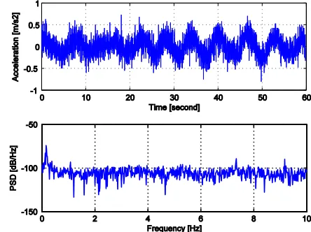
Fig. 3 and Fig. 4 show the time-series of acceleration data their power spectral density (PSD) of the channel ID (1) and (6), respectively. In PSDs, some peaks likely having the modal parameter information including a narrow and sharp peak assumed of harmonics at around 374 Hz are observed.

A. Validating

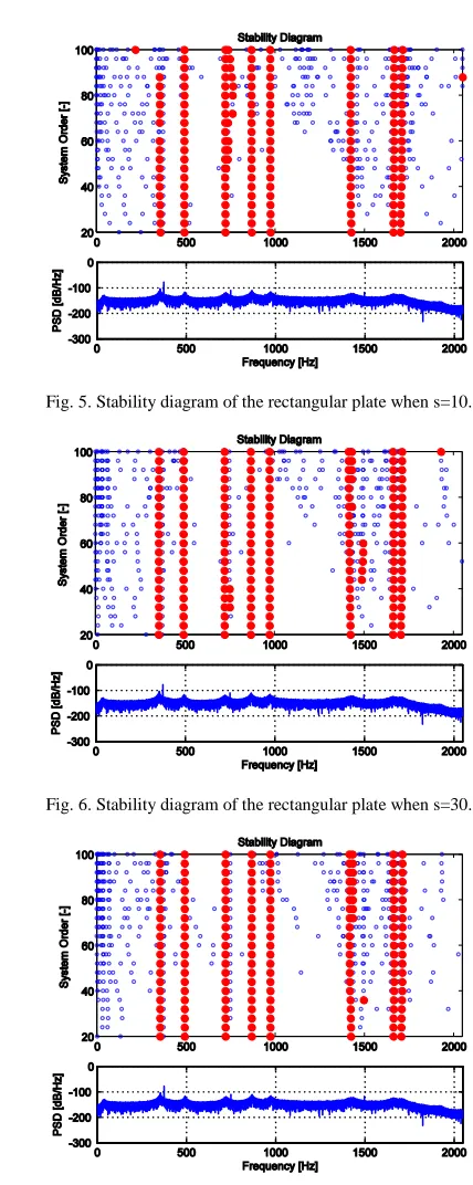
A stability diagram is adopted for verifying the implemented code, which plots the system order versus the modal frequencies, and helps intuitively the quality of the solution. The modal parameters by each system order are extracted via two-step process. First the modal frequencies of all extracted modes are marked on the stability diagram with the hollow small circle. Of them, second, the valid modes are collected from all modes under the pre-defined damping criteria, and marked with the solid large circle. Representatively, Fig. 5 to Fig. 7 show the stability diagrams of the target rectangular plate including the corresponding PSD at the acquisition point (1), where the number of data block 𝑠 is set to 10, 30 and 50, respectively. The system order 𝑚 is from 20 to 100 in step increase of 4 and the frequency range interested is from 0 Hz to

2,048 Hz. The pre-defined damping criteria range from 0.3% to 1.5%. These stability diagrams prove that the solutions are more stable as the number of data block of the block Hankel matrix s and the system order m increase. This shows that the implemented code is operating its function well and could provide stable solutions by determining appropriate parameters.

Fig. 3. Time-series of acceleration data for acquisition point (1) of rectangular plate.

Fig. 4. Time-series of acceleration data for acquisition point (6) of rectangular plate.

Fig. 5. Stability diagram of the rectangular plate when s=10.

Fig. 6. Stability diagram of the rectangular plate when s=30.

B. Verification

For verification of the implemented code, the modal parameters are estimated for the rectangular plate. The system order 𝑚 is fixed to 100 providing stable solutions in the stability diagrams, and the number of data blocks 𝑠 changes from 10 to 50 in the step increment of 10. The damping criteria are same above. The estimated modal frequencies and the modal damping values (Present) are compared with those of ARTeMIS [10] (Reference) in TABLE I and TABLE II, respectively. The implemented code is missing modes corresponding Reference mode number 1, 6 and 8 when the number of data block 𝑠 = 10 and 𝑠 = 20, but finds well the modes for other cases. Fig. 8 shows the percentage deviation of the estimated modal frequency over Reference (=

|[𝑃𝑟𝑒𝑠𝑒𝑛𝑡] − [𝑅𝑒𝑓𝑒𝑟𝑒𝑛𝑐𝑒]|/[𝑅𝑒𝑓𝑒𝑟𝑒𝑛𝑐𝑒] × 100) . The percentage deviation of the modal frequencies are enough low for all cases, of which the maximum value is 0.44% for the reference mode number 7. Fig. 9 shows the deviation of the estimated modal damping against Reference (= |[𝑃𝑟𝑒𝑠𝑒𝑛𝑡] −

[𝑅𝑒𝑓𝑒𝑟𝑒𝑛𝑐𝑒]|). The maximum deviation of the modal frequencies is 0.25 % point both for the reference mode number 7 and 9. When 𝑠 = 50, however, the values decrease 0.13 % point and 0.03 % point respectively. This means that as the number of the block 𝑠 increases, the accuracy improves as mentioned in the above verification. In conclusion, when 𝑠 = 30, 40, 50, the modal frequencies and damping values are estimated with good accuracy.

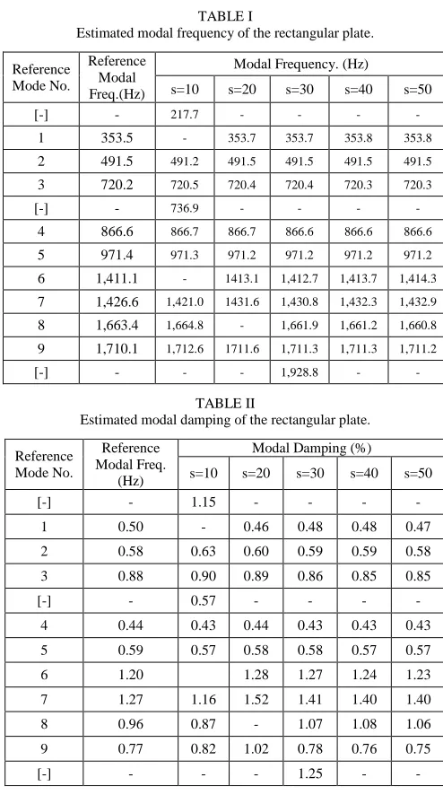
TABLE I

Estimated modal frequency of the rectangular plate.

Reference Mode No.

Reference Modal Freq.(Hz)

Modal Frequency. (Hz)

s=10 s=20 s=30 s=40 s=50

[-] - 217.7 - - - -

1 353.5 - 353.7 353.7 353.8 353.8

2 491.5 491.2 491.5 491.5 491.5 491.5

3 720.2 720.5 720.4 720.4 720.3 720.3

[-] - 736.9 - - - -

4 866.6 866.7 866.7 866.6 866.6 866.6

5 971.4 971.3 971.2 971.2 971.2 971.2

6 1,411.1 - 1413.1 1,412.7 1,413.7 1,414.3

7 1,426.6 1,421.0 1431.6 1,430.8 1,432.3 1,432.9

8 1,663.4 1,664.8 - 1,661.9 1,661.2 1,660.8

9 1,710.1 1,712.6 1711.6 1,711.3 1,711.3 1,711.2

[-] - - - 1,928.8 - -

TABLE II

Estimated modal damping of the rectangular plate.

Reference Mode No.

Reference Modal Freq.

(Hz)

Modal Damping (%)

s=10 s=20 s=30 s=40 s=50

[-] - 1.15 - - - -

1 0.50 - 0.46 0.48 0.48 0.47

2 0.58 0.63 0.60 0.59 0.59 0.58

3 0.88 0.90 0.89 0.86 0.85 0.85

[-] - 0.57 - - - -

4 0.44 0.43 0.44 0.43 0.43 0.43

5 0.59 0.57 0.58 0.58 0.57 0.57

6 1.20 1.28 1.27 1.24 1.23

7 1.27 1.16 1.52 1.41 1.40 1.40

8 0.96 0.87 - 1.07 1.08 1.06

9 0.77 0.82 1.02 0.78 0.76 0.75

[-] - - - 1.25 - -

Fig. 3. Percentage deviation of modal frequency of rectangular plate.

Fig. 4. Deviation of modal damping of rectangular plate.

In addition, the estimated modal vector 𝜑_𝑝 is qualified using modal assurance criteria 𝑀𝐴𝐶𝑝𝑟 over Reference 𝜑𝑟, which is defined by the equation (19).

𝑀𝐴𝐶𝑝𝑟=

|𝜑_𝑝𝑇𝜑_𝑟∗|2

|𝜑_𝑝𝑇_𝜑𝑝∗_||𝜑𝑟𝑇_𝜑𝑟∗_| (20)

where (∙)∗is the complex conjugate operator.

Fig. 10 plots the MAC value matrices of the modal vectors between Present and Reference. The MAC values shows higher as the number of data blocks increases. In conclusion, when 𝑠 = 30, 40, 50, the modal vectors are estimated with good accuracy. Thus the implemented code has been verified in terms of the accuracy by comparing with the commercial S/W.

IV. APPLICATION TO SHIP STRUCTURE

A. Target ship and data acquisition

In order to investigate applicability of the present to ship structures, the modal parameter of an oil tanker is estimated by using the implemented code, of which the size is around the length overall of 180 m, the beam width of 32 m, the depth of 19m and the displacement of around 50,000 tons in full load condition. The data has been measured using a data acquisition and signal analyzer (B&K Pulse 3560D) on the target ship running a straight course during sea trials. For reference, she has a diesel engine and a 4-bladed fixed-pitch propeller which have been operated the speed of 110 revolutions per minute during measurement. The excitation harmonics by diesel engine and the propeller might be observed in the corresponding speed, which are summarized in TABLE III. By considering the interesting frequency range to 10Hz, the harmonics of 1.83 Hz, 3.67 Hz, 5.50 Hz, and 7.33 Hz, have to be referred in modal parameter estimation of the target ship. The time-series data sets have been gathered via the 12 channels connected to the accelerators (Dytran 31148D) which are attached onto the points and toward the directions shown in

Fig. 11.

B. Data set sampling

The data sets used in this study have been sampled in 64 Hz during 60 seconds, where the sampling frequency corresponds to the Nyquist frequency of 32 Hz and has been determined by considering the interesting frequency range to 10 Hz. Fig. 12 and Fig. 13 show the time-series of the sampled acceleration and the PSD at the channel 1 and 10, representatively. In Fig. 12, outstanding peaks are observed in 0.16 Hz, 1.08 Hz, 3.67 Hz, 5.50 Hz, 7.34 Hz, 9.17 Hz, etc.

C. Modal parameter estimation

As mentioned in validations above, as the parameter such as the system order and the number of the block increase, the accuracy improves, but computational cost also increases. Accordingly, the appropriate parameter has to be selected for cost-effective modal parameter estimation. In this application, the number of the block 𝑠 is fixed to 100 and the estimated modal parameters of the target ship are observed with a stability diagram when the system order changes 10 to 200 in the step increase of 10, where the pre-defined damping criteria range from 0.3% to 5.0%. The stability diagram of the target ship shown in Fig. 14 suggests that modal parameters would exist at the 0.17 Hz, 1.07 Hz, 3.49 Hz, 4.39 Hz, 4.70 Hz, 5.34 Hz, 7.20

TABLE III

Harmonics by diesel engine and propeller of target ship (@110 rpm).

Order 1 2 3 4 5 6

Freq (Hz)

Engine &

propeller 1.83 3.67 5.50 11.00 16.50 33.00 Propeller

blade 7.33 14.67 22.00 44.00 66.00 132.0

Fig. 6. Measuring point on target ship, channel identification number, and accelerometer direction.

Fig. 7. Time-series of sampled acceleration data and PSD (Channel 1).

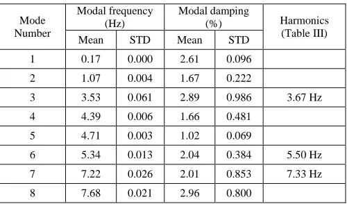
Hz and 7.66 Hz within the interesting frequency range. For more precise modal parameter estimation of the target ship, the modal frequencies and modal damping values are listed together in TABLE IV and TABLE V. The mode number of each the system order is matched onto the last one (Reference, 𝑚 = 200) by checking similarity of the modal frequency. Then valid modes are selected by evaluating MAC values over the modal vectors of Reference, where the invalid modal parameters having MAC value less than 0.9 are within the parenthesis on the tables. Finally, the modal parameter of the target ship is estimated by averaging them in case that valid modes exists more than two on the same system order. The finally 8 estimated modal parameters of the target ship are summarized in TABLE VI with the standard deviation STD.

Unfortunately, the modes (mode number 3, 6 and 7) are nearby the harmonics in TABEL III, which means that the estimated modal parameter for the corresponding modes might be garbage by harmonics from forcing vibration by the diesel engine or the propeller. This ambiguity could be checked with the results in other speed condition later.

V. CONCLUSION

The mathematical formulation of data-driven SSI has been summarized and a code has been implemented for the modal parameter estimation of the ship structure. The implemented

code has been verified and validated through the benchmark test of a rectangular plate, where the modal parameters have been estimated by changing key parameter such as the system order and the number of the block, and the results have been compared with those of the commercial software. The benchmark test has shown that the implemented code operates well its function and provides stable solution by selecting appropriate parameters and as the key parameter such as the system order and the number of the block increase, the accuracy improves. Then the implemented code has been applied for estimating the modal parameter of an oil tanker, where the data sets used have been sampled from acceleration data measured during her sea trial and 8 modes have been found by averaging the valid modal parameters evaluated with damping criteria and modal assurance criteria. This shows that the implemented code is applicable to large built-up structure like ship structures. Nevertheless, case studies are required for various operation conditions as a future works.

ACKNOWLEDGMENT

This research was supported by the Tongmyong University of Research Grants 2014(2014A010).

REFERENCES

[1] Avitabile, P. (2001). Experimental Modal Analysis: A Simple Non-mathematical Presentation, Sound and Vibration Magazine, 1–11. [2] Rainieri, C. and Fabbrocino, G. (2014), OperationalModal Analysis of

Civil Engineering Structure, Springer.

Fig. 9. Stability diagram of target ship.

TABLE IV

Estimated modal frequencies of target ship.

Mode Number

System order m

140 150 160 170 180 190 200*

1 0.17 0.17 0.17 0.17 0.17 0.17 0.17

2 1.06 1.06 1.07 1.07 1.07 1.07 1.07

3 3.60 (3.60) (3.56) (3.51) (3.51) 3.50 3.49

4 (4.41) (4.41) (4.40) 4.38 (4.39) 4.39 4.39

5 4.71 4.71 4.71 4.71 4.70 4.70 4.70

6 5.36 5.34 5.32 5.33 5.33 5.33 5.34

7 - - - - 7.23 (7.24) 7.20

8 - (7.77) (7.78) (7.75) (7.78) 7.69 7.66

9 - - - (9.27)

( ): Invalid mode of which MAC value less than 0.9, *: Reference case

TABLE V

Estimated modal dampings of target ship

Mode Number

System order m

140 150 160 170 180 190 200*

1 2.58 2.73 2.69 2.70 2.52 2.51 2.53

2 1.98 2.01 1.49 1.56 1.61 1.54 1.53

3 3.98 (4.44) (4.36) (4.20) (3.05) 2.64 2.06

4 (3.21) (2.32) (1.99) 2.19 (1.61) 1.51 1.26

5 1.04 1.01 1.02 0.95 0.96 1.01 1.16

6 2.76 2.23 2.11 1.98 1.82 1.83 1.56

7 - - - - 2.61 (1.93) 1.40

8 - (4.51) (3.70) (2.90) (2.48) 3.53 2.40

9 - - - (3.59)

( ): Invalid mode of which MAC value less than 0.9, *: Reference case

TABLE IVI

Finally estimated modal parameters of target ship.

Mode Number

Modal frequency (Hz)

Modal damping

(%) Harmonics (Table III) Mean STD Mean STD

1 0.17 0.000 2.61 0.096

2 1.07 0.004 1.67 0.222

3 3.53 0.061 2.89 0.986 3.67 Hz

4 4.39 0.006 1.66 0.481

5 4.71 0.003 1.02 0.069

6 5.34 0.013 2.04 0.384 5.50 Hz

7 7.22 0.026 2.01 0.853 7.33 Hz

[3] Rosenow, S. E., Meinke, K. D. and Schlottmann, G. (2005), Investigation of the dynamic of ship structures using classical and operational modal testing, in Proc. IOMAC 2005, 288-294

[4] Batel, M. (2002), Operational Modal Analysis – Another way of doing modal testing, Sound and Vibration Magazine, 22–27.

[5] Bertha M., and Golinval, J. C. (2016), Multivariate ARMA Based Modal Identification of a Time-varying Beam, Topics in Modal Analysis &

Testing, Volume 10, 273-280.

[6] Pavlov, G. K. (2008), Design of Health Monitoring System to Detect Tower Oscillations, M. Thesis, Tech. Univ. of Denmark.

[7] Overschee, P. V. and Moor, B. D. (1996), Subspace Identification for

Linear Systems, Kluwer Academic Publishers.

[8] Dohler, M., Andersen, P. and Mevel, L. (2012), Operational modal analysis using a fast stochastic subspace identification method , Topics in

Modal Analysis I, Volume 5, 19-24.

[9] Londono, N. A., Desjardins, S. L. and Lau, D. T. (2004), Use of stochastic subspace identification methods for post-disaster condition assessment of highway bridges, in Proc.13 WCEE, paper No. 2714.