Von Neumann Stability Analysis of Reduced Navier-Stokes
Equations in Vorticity-Stream Function Formulation
T.M.Shah∗, N.Talat† Department of Mathematics,
Air University Islamabad
Abstract
In [1, 2] Fourier Stability Analysis of Navier-Stokes Equations has been carried out,where non-linearity were incorporated by freezing non-linear terms and obtained optimum smoothing factors which were in a close agreement with practical smoothing factors. In this paper an effort was made to obtain Von-Neumann stability of elliptic type reduced Navier-Stokes equations in vorticity-stream function formu-lation. Using stream function in cartesian coordinate system we derived the Vorticity transport equation by eliminating pressure term from momentum equa-tions in cross differentiation. The derived equation is classified as a parabolic equation with the unknown vorticity ,ω. By considering the definition of the vor-ticity, we derived the equation known as the stream function equation and is classified as elliptic PDE with the unknown stream function ,ψ. The stability analysis is carried out by converting stream function equation expressed in non-dimensional form so that the non-linearity is vanished in the equation. With the induction of vorticity and stream function,the in-compressible Navier-Stokes equations are decoupled into one elliptic and one parabolic equation. The Von Neumann stability analysis is carried out for the ellip-tic equation only. The various numerical experiments using iterative schemes have been carried out to
ob-are plotted for amplification factors for a number of unknown parameters.
1
Navier-Stokes Equation
Incompressible and unsteady Navier-Stokes Equa-tions in cartesian forms are as follows:- Continuity
Equation:-∂u ∂x+
∂v
∂y = 0 (1)
Momentum Equations without external force term:-∂u
∂t +u ∂u ∂x+v
∂u ∂y =−
1 ρ ∂p ∂x + µ ρ(
∂2u ∂x2 +
∂2u ∂y2) (2) ∂v
∂t +u ∂v ∂x +v
∂v ∂y =−
1 ρ ∂p ∂y + µ ρ(
∂2v ∂x2 +
∂2v ∂y2) (3)
2
Vorticity-Stream
Function
Formulation
u=b∂ψ ∂y
The Vorticity Equation is
ω= ∂v ∂x −
∂u
∂y (4)
In order to derive the vorticity transport equation, pressure is eliminated from momentum equations by cross differentiation. Differentiation with respect to y of equation(2) yields
∂2u ∂y∂t+
∂u ∂y
∂u ∂x+u
∂2u ∂x∂y +
∂v ∂y
∂u ∂y +v
∂2u ∂y2 =
−
1 ρ
∂2p ∂x∂y +
µ ρ(
∂3u ∂y∂x2 +
∂3u ∂y3) (5) whereas the differentiation with respect to x of equa-tion(3) yields
∂2v ∂x∂t +
∂u ∂x
∂v ∂x +u
∂2v ∂x2 +
∂v ∂x
∂v ∂y+v
∂2v ∂x∂y =
−
1 ρ
∂2p ∂x∂y +
µ ρ(
∂3v ∂x3 +
∂3v
∂x∂y2) (6) subtracting equation(6) from equation(5) to obtain [3]
∂ω ∂t +u
∂ω ∂x +v
∂ω ∂y =
µ ρ(
∂2ω ∂x2 +
∂2ω
∂y2) (7) The vorticity equation can be reduced into
a∂ 2ψ
∂x2 +b ∂2ψ
∂y2 =−ω (8)
3
Non-dimensionalization
Equation(7) and equation(8) can be non-dimensionalized by using the following substitutions Ω = ωL
u∞ ,X =
x L,Y =
y L ,T=
u∞t
L
u= u u∞,v=
v v∞ ,
1
Re = µ
ρu∞L ,ψ=
ψ u∞L
Equation(7) implies that ∂Ω
∂T +u ∂Ω ∂X +v
∂Ω ∂Y =
1 Re(
∂2Ω ∂X2+
∂2Ω ∂Y2) (9) Equation(8) implies that
a∂ 2ψ
∂X2 +b ∂2ψ
∂Y2 =−Ω (10)
Equations (9) and (10) are reduced parabolic and el-liptic respectively. For the seek of stability analysis, we consider equation(10) only.
4
Stability Analysis for Stream
Function Equation
The Finite Difference Formulation for equation (10) is as
follows:-aψi+1,j−2(a+b)ψi,j+aψi−1,j+bψi,j+1+bψi,j−1=−h
2Ω
i,j
(11) By applying Jacobi iterative method, we get
aψik+1,j−2(a+b)ψi,jk+1+aψik−1,j+bψ k
i,j+1+bψki,j−1=−h
2Ω
i,j
(12) Subtracting equation(12) from equation (11) we get aeki+1,j−2(a+b)eki,j+1+ae
k
i−1,j+be k
i,j+1+beki,j−1= 0
(13) Letek
i,j=A(θ, φ)eι(iθ+jφ)
After substitution in equation(13) and simplifica-tion , we get amplificasimplifica-tion factor as
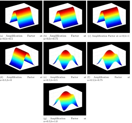
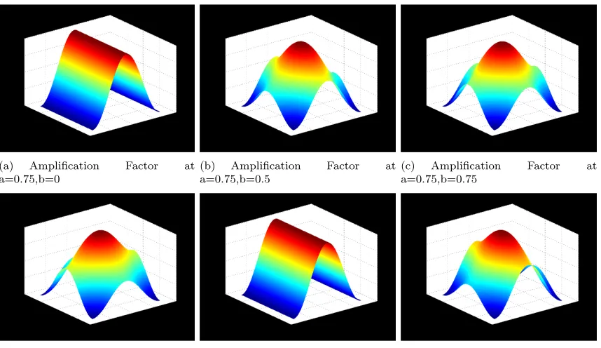
follows:-G(θ, φ) = AA¯((θ,φθ,φ)= acosθa++bbcosφ
The Finite Difference Formulation for equation (10) is as
follows:-aψi+1,j−2(a+b)ψi,j+aψi−1,j+
bψi,j+1+bψi,j−1=−h
2Ω
i,j (14)
By applying Gauss-Seidel iterative method, we get aψki+1,j−2(a+b)ψki,j+1+aψ
k+1
i−1,j+
bψi,jk +1+bψi,jk+1
−1=−h
2Ω
i,j (15)
Subtracting equation(15) from equation (14) we get aeki+1,j−2(a+b)eki,j+1+ae
k+1
i−1,j+be k
i,j+1+beki,j+1−1= 0
(16) Leteki,j=A(θ, φ)eι(iθ+jφ)eki,j+1= ¯A(θ, φ)eι(iθ+jφ) Af-ter substitution in equation(16) and simplification , we get amplification factor as
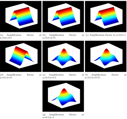
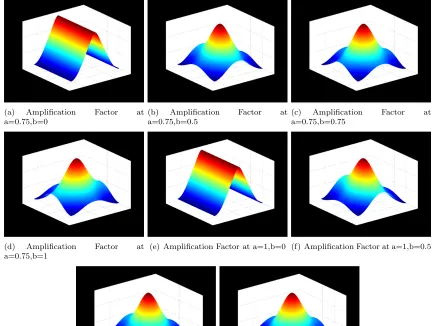
follows:-G(θ, φ) =A¯(θ, φ) A(θ, φ) =
aeιθ+beιφ
2a+ 2b−ae−ιθ−be−ιφ
(17)
5
Results and discussions
The main purpose of Von Neumann stability analy-sis [3] has been to assess the smoothing factor of it-erative schemes,Jacobi and Guass-Seidel methods for reduced Navier-Stokes equations.The Von Neumann stability analysis was carried out for Stream Func-tion only.In order to analyze non-linear formulaFunc-tion of stream function equation we defined u and v veloc-ities with the multiple of constant coefficient a and b multiplied by differentials of stream function in both x and y coordinates. This made the stream func-tion formulafunc-tion non-linear in non-dimensional form. Both constants a and b varies between (0,1). There-fore we carried out Von Nuemann stability analysis of non-linear stream function equation and effectively
found that the maximum smoothing factor for Ja-cobi Iterative scheme are for a=0 and for all values of b except zero and for all values of a except zero with b=0, and for all other combination of values of a and b lies below the maximum. Figure 2 shows the smoothing factor for various values of a and b and it was also found that the maximum smoothing factor for Gauss-Seidel, although lesser than Jacobi methods behaves in similar way that is for a=0 and for all values of b except zero and for all values of a except zero with b=0. The similar behavior is found for other values of a and b but lies below the max-imum. This analysis concluded that if the reduced Navier-Stokes are solved by the described iterative scheme solution is guaranteed. The Von Neumann stability analysis may also be carried out for other formed of reduced Navier-Stokes equations, like vor-ticity transport formulation similar to this analysis. Further this analysis can also be done for other iter-ative scheme. A thorough compariter-ative analysis of all iterative scheme will be done in future work.
References
[1] T.M.Shah, N.Talat, Three Dimensional Analysis and Application of A Line Solver for the Recir-culating Flows Using Multi-grid Methods. to be published in IJEIT.
[2] T.M.Shah,D.F.Mayers,and J.S.Rollett. Analysis and Application of A Line Solver for the Recirculating Flows Using Multigrid methods. In R.Rannacher W.Hackbusch,editor,Numerical Treatment of the Navier-Stokes Equations,pages 134-144,Braunschweig,January 1990.Vieweg.
[3] Klaus A. Hoffmann and Steve
(a) Amplification Factor at a=0,b=0.5
(b) Amplification Factor at a=0,b=0.75
(c) Amplification Factor at a=0,b=1
(d) Amplification Factor at a=0.5,b=0
(e) Amplification Factor at a=0.5,b=0.5
(f) Amplification Factor at a=0.5,b=0.75
(g) Amplification Factor at a=0.5,b=1.0
(a) Amplification Factor at a=0.75,b=0
(b) Amplification Factor at a=0.75,b=0.5
(c) Amplification Factor at a=0.75,b=0.75
(d) Amplification Factor at a=0.75,b=1
(e) Amplification Factor at a=1,b=0 (f) Amplification Factor at a=1,b=0.5
(g) Amplification Factor at a=1,b=0.75
(h) Amplification Factor at a=1,b=1
(a) Amplification Factor at a=0,b=0.5
(b) Amplification Factor at a=0,b=0.75
(c) Amplification Factor at a=0,b=1
(d) Amplification Factor at a=0.5,b=0
(e) Amplification Factor at a=0.5,b=0.5
(f) Amplification Factor at a=0.5,b=0.75
(g) Amplification Factor at a=0.5,b=1
(a) Amplification Factor at a=0.75,b=0
(b) Amplification Factor at a=0.75,b=0.5
(c) Amplification Factor at a=0.75,b=0.75
(d) Amplification Factor at a=0.75,b=1
(e) Amplification Factor at a=1,b=0 (f) Amplification Factor at a=1,b=0.5
(g) Amplification Factor at a=1,b=0.75
(h) Amplification Factor at a=1,b=1