Adaptive Numerical and Computational Methods for Temperature Profiling of a Cylindrical Nuclear Fuel Rod



Abstract—Accurate prediction of temperature profile of the fuel rod in a nuclear reactor is very important due to safety factors. Temperature at the center and at the surface is critical for designing a nuclear fuel rod. The cladding of the fuel rod is done to incresase the physical strength of the Fuel Rod. The temperature distribution in steady state operation in the nuclear reactor is determined by thermal balance between heat generated and heat transferred to the coolant. This paper attempts a numerical solution to the heat transfer problem of a cylindrical nuclear fuel rod with cladding having uniform generation throughout the fuel body, and heat transfer taking place through convection and radiation at the lateral surface of the cladding material. Solutions proposed through various computational methods i.e. Finite Difference Method (FDM), Finite Volume Method (FVM) and Finite Element Method (FEM) . These results have been plotted and a comparative analysis has been considered to arrive at a desired exactness of the solution. The calculated values from each of the methods are compared and analyzed; appropriate reasons for the deviation of the computed result from the exact solution have been explained.

Index Terms—FDM, FVM, FEM, radiation, cladding.

I. INTRODUCTION

Temperature profile of a nuclear fuel rod can be well defined using different numerical methods with appropriate boundary conditions. Antar [1] offered a simplified numerical solution of unsteady heat conduction problem in a short cylinder. In this paper, solutions to a mixed boundary heat flow problem (convection and radiation) in nuclear rod with cladding have been proposed and compares the result obtained in each method [2], [3] for different meshes. Nuclear energy is energy released from the nuclear fuel in the form of heat energy which is finally converted into electricity energy. Nuclear fuel is any material that can be consumed to derive nuclear energy. The most common fissile nuclear fuels are enriched uranium or plutonium in the form of pencil-thin cylindrical rods which are stacked inside tubes. Othman[4] has studied the nuclear fuel rod with cladding in transient condition.

The cladding prevents the escape of fission products to the coolant. Zirconium alloys have been used in a number of water–cooled fission reactor types due to their excellent aqueous corrosion resistance, low thermal neutron absorption cross section and good mechanical properties.

Manuscript received August 10, 2013; revised December 20, 2013. The authors are with the S‟O‟A University, Department of Mechanical Engineering, ITER, Bhubaneswar, Odisha, India (e-mail:

[email protected], [email protected],

[email protected], [email protected], [email protected], [email protected]).

The finite difference method (FDM) [5] is based on the differential equation of the heat conduction, which is transformed into a difference equation. The temperature values are calculated at the nodes of the network. Using this method, convergence and stability problem can appear. Han

et al., [2] used FDM method with FEM for analysis of one-dimensional fin.

Dhawan et al., [6] studied the heat conduction problem in an aluminium plate using finite element method and got very good results compared to the exact solution. The finite element method (FEM) is based on the integral equation of the heat conduction. This is obtained from the differential equation using variational calculus. In first case the temperature values are calculated on the finite elements. Then, based on these partial solutions, the solution for the entire volume is determined. Using this method the whole surface has been divided into elements and fields with unregulated border [7], [8]. In this paper the temperature distribution is analyzed in the radial direction of a solid cylinder. The practical application is in the electrical wires where heat is generated in the wire and the same heat it needed to be dissipated to the surrounding so that the melting of the wire is avoided.

The desired properties of the nuclear fuel rod are that they must be fissionable [9], [10], should have high thermal conductivity, corrosive resistant, good mechanical strength at high temperatures and high limiting temperature for operation.

This paper presents the thermal analysis in a cylindrical nuclear fuel rod having isotropic physical characteristics [11] [12]. Uniform heat generation is assumed from the entire body and with convection and radiation through the lateral surface. Any kind of heat conduction in axial direction is neglected.

II. THEORY

The general 3-D heat conduction problem with generation and time varying follows the equation (1) below:

2 2 2

2 2 2

T T T T

k g C

x y z



t

 _ _ _{ } 

_{  }  _

 

(1)

In our problem we have a cylinder with radial conduction and no conduction through the axial direction [13]. Hence, our problem is limited to 1-Dimesional radial conduction which is given by equation (2) below:

1

T

T

k

r

g

C

r r

r



t

 





_{  }







_



_

_



_



_





(2)

Adaptive Numerical and Computational Methods for

Temperature Profiling of a Cylindrical Nuclear Fuel Rod

In steady state the governing differential equation for cylindrical coordinate system with uniform internal heat generation is given in equation (3):

1

0

T

g

r

r r

r

k







_{  }













(3)

III. BOUNDARY CONDITION

Symmetric Boundary Condition:. at r_=0,

dT

0

dr



Robbin‟s Boundary Condition with Radiation: at r=r2,







4 4



B B

dT

k

h T

T

T

T

dr













 



Interface Boundary Condition: At r = r1,

f c

dT

dT

k

k

dr

dr



 

Exact Solution

The exact solution has been solved in two parts. First, the fuel rod part is considered i.e. with generation and the general equation is found. Second, the cladding part of the fuel rod is considered i.e. without generation and the graph is obtained by merging both the results.

The final equation followed by the temperature profile is as follows:

For 0 < r < r1





2 2

2 2

1 1 2

1 2

ln

2

2

_c

4

_f

gr

gr

r

g

T

T

r

r

r h

k

r

k



 







_{ }





 

(4)

For r1< r < r2

2 2 1 1 2

ln

ln

2

2

B c c

gr

gr

T

T

r

r

k

k







(5)

where TB is the surface temperature and can be found from

the Boundary condition









2

4 4

c B B

r

dT

K

h T

T

T

T

dr

 













ò



(6)

Hence we found that the above equation can be modified into:

2

4 1 4

2

2

B B

r g

E

T

h T

h T

T

r



_{  }



_



ò







 

(7)

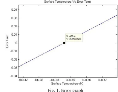
Here E represents the Error term. Hence when we have the error term E=0 then we have the solution for the above bi-quadratic equation. The following graph gives us the value of the surface temperature (TB), which is coming as 400.4 K

with the error term as 0.0001601 which can be assumed to be 0. The given graph (Fig.1) has been plotted using Matlab and hence to make error exactly equal to 0 is difficult. Since the value of error tending to 0, we assume that the value of temperature will remain unaffected by this small error.

Fig. 1. Error graph

IV. NUMERICAL ANALYSIS

FDM: FDM is based on the governing differential equation, which is transformed into a difference equation using FD [14], [15] M. The element is divided into nodes (Fig. 2).

Fig. 2. FDM domain

For node i=1:

2

1

4

i

4

i

g r

T

T

k









(8) For node i=2 to m-1,

when r < r1:









2

1 1

1 1

2 1 1

2 1 2 1

i i i

g r

T T T

i  i  k

    

 _{ } _  _{ } _ 

   

(9)

when r = r1

1 1 i 1

i i 1

2 2

k

k T

1

T

T

k

k

 































(10)

when r > r2





1





1

1

1

2

1

1

2

1

2

1

i i i

T

T

T

i



i











 



_



_

 



_



_













(11) For node i=m,

4

1

3 4

1

4 iS m m 3 iS

h r h r T r

k k k

T T

rT T r

k k







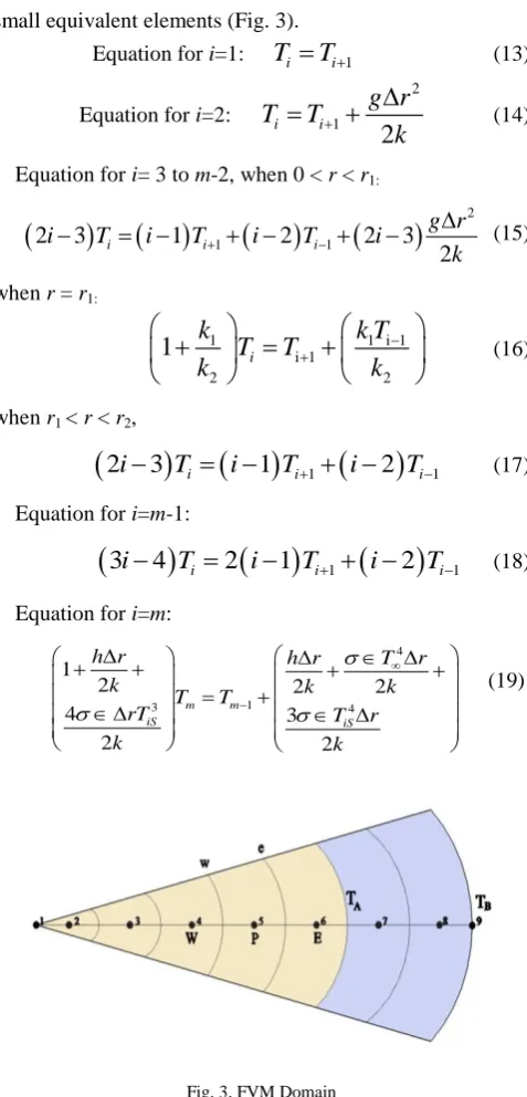
         _{ }  _{ }                           (12)

small equivalent elements (Fig. 3).

Equation for i=1:

T

_i



T

_i1 (13) Equation for i=2:

2

1

2

i i

g r

T

T

k









(14)

Equation for i= 3 to m-2, when 0 < r < r1:



2

3



 

1

1



2



1



2

3



2

2

i i i

g r

i

T

i

T

i

T

i

k

 





 

 





(15)

when r = r1:

1 1 i 1

i 1

2 2

1

k

T

_i

T

k T

k

k

 































(16)

when r1 < r < r2,



2

i



3



T

i

 



i

1



T

i1

 



i

2



T

i1 (17)

Equation for i=m-1:



3

i



4



T

i



2



i



1



T

i1

 



i

2



T

i1 (18)

Equation for i=m:

4

1

3 4

1

2 2 2

4 3

2 2

m m

iS iS

h r h r T r

k _{T T} k k

rT T r

k k



 







    

 _{ }  _{ }

 

 

 

   

    

 

   

  





(19)

Fig. 3. FVM Domain

FEM: Finite Element Method is another method for numerical solution of the differential equation. ANSYS 13.0 well established commercial software is used in this paper for required analysis and the details are produced in the results and discussion section. Some of the important steps followed for FEM analysis are as follows:

1) Geometry designing: The analysis was done on a cylinder of radius 0.05 meters and cladding of thickness 0.02 meters and sufficient length was provided to neglect the axial heat conduction.

2) Loading: The lateral surface was provided mixed boundary condition i.e. convection and radiation simultaneously. In order to obtain a better result the end surfaces were insulated.

3) Meshing: The cylinder rod is now divided into number of hexahedral meshes as shown in Fig5b. The finest possible mesh was used so as to obtain results closer to the actual analysis.

4) Solution: The meshed and the loaded geometry were

solved using the ANSYS solver. In this step ANSYS solves the problem under required conditions.

5) Post-Processing: The results obtained by the ANSYS solver are viewed in this step. The temperature and flux contours can be seen here.

V. SOLUTION TECHNIQUES

A. Gauss Seidel Iteration

The FDM and FEM solution both results in a set of algebraic equations which are required to be solved simultaneous. The set of equations can be solved by matrix formation however; alternative method of Gauss-Seidel iteration technique is applied. This technique requires less computational effort and hence is preferred. Here we have a reasonable guess value for the temperature at each node. The temperature of a node is related to the temperature around it. Hence we solve the equation is a logical order using the current value of the temperature of the surrounding node. The difference between the original and recalculated value of each temperature is computed and the maximum value of this error is recorded for each iteration. The iteration is repeated unlit the numerical error associated with the iteration is less than some tolerance limit.

B. Source Term Linearization

In radiation heat transfer, the source term is energy equation expressed as fourth power in temperature. Source term A. (.  in the problem (equation 20) is a bi-quadratic equation and hence linearization is applied to make the equation linearized as follows:

4

B

S

 



T

(20) By source term linearization





* *

B B

dS

S

S

T

T

dT









_

_







(21)

Here Superscript „*‟ correspond to the old value of the node or node center.





*4 *3 *

4

B B B B

S

 



T







T

T



T

(22)

Therefore





T

_B4

 



3





T

_B*4

 



4





T

_B*3



T

_B Hence, the mth node equation in FDM and FVM solution having the term T4 is substituted by the term



*4

 

*3



3



T

_B

4



T

_B

T

_B









hence linearizing the

bi-quadratic equation and giving simpler solution.

VI. RESULT AND DISCUSSION

tabulated (Table I) and the parameters used in Table II. The nomenclature is mentioned in Table III:

TABLEI:RADIAL TEMPERATURE DISTRIBUTION

Radial Distance FDM FVM Exact FEM

0 458.3 460.2 459.0 459.0

0.01 456.5 458.3 457.1

0.02 450.8 452.4 451.3

0.03 441.3 442.5 441.7

0.04 427.9 428.6 428.2

0.05 410.7 410.7 410.9

0.06 405.1 405.2 405.2

0.07 400.4 400.4 400.4 400.4

TABLEII:PARAMETER AND VALUES USED

Serial

No. Parameter Value

1 Radius of fuel rod (m) 0.05

2 Thickness of cladding material (m) 0.02

3 Generation (W/m3_{) 10}6

4 Thermal conductivity of fuel rod (W/mK) 13

5 Thermal Conductivity of cladding material

(W/m2_K) 40

6 Convective Heat transfer C-efficient (W/m2_{K) 40,000}

7 Emissivity 0.8

8 Ambient Temperature (K) 400

9 Stefan Boltzmann Constant (W/K4) 5.67x10-8

Following are the solution obtained by using ANSYS.

Fig. 4 (a). Temperature contour

Fig. 4 (b). Meshing

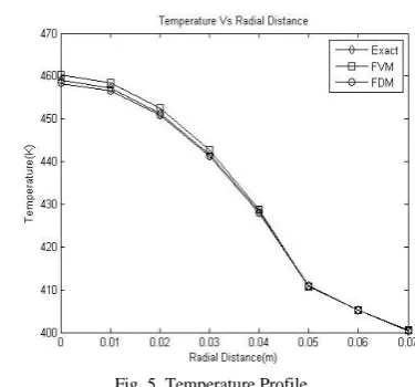
The FDM and the FVM solutions divert from the exact solution because 1st order accurate equations has been used on the boundary and 2nd accurate equations has been used at the centre. If equations of higher order of accuracy is used the FDM and FVM solutions can be closer to the exact solution. The FEM solution can be made more accurate with the use of

finer meshes.

Fig. 5. Temperature Profile

It can be seen that maximum temperature is obtain at the core of the Fuel rod and the minimum temperature in obtained at the outer surface of the cladding material. The cladding prevents the Fuel Rod from physical damage. Hence appropriate thickness of cladding material has to be used in order to have safe operation of the Nuclear Fuel Rod.

VII. CONCLUSION

This paper has presented various computational techniques involved in a thermal problem. The numerical solution with FEM, FDM and FVM represent an efficient way of obtaining temperature profile for a steady state Conductive and Radiation heat transfer process. FDM, FEM and FVM methods can be involved for solving any complex body by breaking the body into small domains. Also, choice of finer grids which requires high computing capability can remove approximation errors to larger extent. Further optimization of the thickness of the cladding can be done considering the relative thermal conductivity of the fuel to cladding.

NOMENCLATURE

TABLEIII: NOMENCLATURE Symb

ols Parameters Unit

r1 Radius of fuel rod M

r2 Radius of fuel rd with cladding M

h Convective heat transfer co-efficient W/m2_K

kc Thermal Conductivity of cladding material W/mK

kf Thermal Conductivity of fuel rod W/mK

g Generatin Term W/m3

c Specific heat Capacity kJ/kgK

 Stefan Bltzmann Constant W/m2K4

 Emissivity Unitless

TB Surface Temperature K

i Node Number Unitless

REFERENCES

International Journal of Mechanical Engineering Education, vol. 28, no. 3, pp.201-212, 1999.

[2] Y. M. Han, J. S. Cho, and H. S. Kang, “Analysis of a one-dimensional fin using the analytic method and the finite difference method,” J. KSIAM, vol.9, no.1, pp. 91-98, 2005.

[3] B. L. Wang and Y. W. Mai, “Transient one dimensional heat conduction problems solved by finite element,” International Journal of Mechanical Sciences, vol. 47, pp. 303-317, 2005.

[4] Steady State and Transient Analysis of Heat Conduction in Nuclear Fuel Elements: ROZHGAR OTHMAN, KTH Numerical Analysis and Computer Science.

[5] M. N. Ozisik, Finite Difference Methods in Heat Transfer, CRC Press, 2000.

[6] S. Dhawan and S. Kumar, “Comparative study of numerical techniques for 2D transient heat conduction equation using finite element method,” International Journal of Research and Reviews in Applied Sciences, vol. 1, pp.38-46, 2009.

[7] H. K. Versteeg and W. Malalasekera, An introduction to Computational Fluid Dynamics, Longman,1996.

[8] S. V. Patankar, Numerical Heat Transfer and Fluid Flow, Hemisphere Publishing Corporation, Taylor & Francis Group, New York. 1980. [9] E. A. Hoffman and W. M. Stacey “Nuclear Design and analysis of the

fusion transmutation of waste reactor,” Fusion Science and Technology, vol. 45, Jan. 2004.

[10] T. Fukano, S. Mori, S. Akamatsu, and A. Baba, “Relation between temperature fluctuation of a heating surface and generation of drypatch caused by a cylindrical spacer in a vertical boiling two-phase upward flow in a narrow annular channel,” Nuclear Engineering and Design, vol. 217, pp. 81-90.

[11] Z. V. Stosic, “Thermal equivalent between nuclear fuel rod model and ewperimental heater simulator,” Nuclear Engineering and Design, vol. 236, no. 14-16, pp. 1445-1738, August 2006.

[12] B. Cesna, “Analytical model for calculation of the thermo hydraulic parameters in a fuel rod assembly,” Nuclear Engineering and Design, vol. 240, pp. 3708-3715, 2010.

[13] A. H. Malik, M. S. I. Alvi, S. Khushnood, F. M. Muhouz, M. K. K. Ghauri, and A. Shah, “Experimental study of conjugate heat transfer within a bottom heated vertical concentric cylinder enclosure,”

International Journal of Heat and Mass Transfer, pp. 695-719, 2011. [14] Y. M. Han, J. S. Cho, and H. S. Kang, “Analysis of a one-dimentional

fin using the analytic method and the finite difference method,”

J.KSIAM, no. 1, pp. 91-98, 2006.

[15] T. M. Chen and C. C. Chen, “Numerical solution for the hyperbolic heat conduction problems in the radial-spherical co=ordinate system

using a hybrif Greens‟s function method,” International Journal of Thermal Sciecnces, vol. 49, pp. 1193-1196, 2010.

N. Anand was born in Jamshedpur, India on 12th

October 1989. He received B. Tech degree in mechanical engineering from Institute of Technical Education and Research, under Siksha „O‟ Anusandhan University, Odisha, India.

He has keen interest in heat transfer and computational fluid dynamics. He has undergone training at escorts construction equipments, ballabghar, Haryana and at National Thermal Power Corporation of India, Badarpur, India.

P. Acharya was born in Bhubaneswar, Odisha in 1990, he received B.T ech in mechanical engineering of 2008-12 Batch at institute of technical education & research, under Siksha „O‟ Anusandhan University, Bhubaneswar (Odisha), India. He has undertaken Industrial training at Vishakhapatnam Steel plant, vizag & vocational training at integrated Test Range, Chandipur. He has completed a certified course on finite element Analysis using Ansys with Iter & collaboration with IFS academy, Pune. Apart from this he has also completed a Course on Pro-E, at Central Room & Training Centre, Bhubaneswar. He has keen interest in heat transfer, gas dynamics and computational fluid dynamics.

N. Parmar was born in Bhubaneswar, India in 1990, who is pursuing B.Tech in mechanical engineering at Institute of Technical Education and Research, under Siksha „O‟ Anusandhan University, Bhubaneswar, Odisha, India.

She has undergone training on CATIA at central room & training centre, bhubaneswar and Ansys with IFS Academy, Pune. She has also undergone industrial training at HINDALCO, Sambalpur, Odisha, India. She has interest in Heat Transfer and ANSYS Modeling.