Abstract--
A hybrid technique consisting of moving least square differential quadrature and finite difference methods is employed to examine bending problems of irregular composite plates. Based on a transverse shear theory, the governing equations of the problem are derived. The transverse deflection and strain rotations of the plate are independently approximated with moving least square approximations. The partial derivatives of these quantities, at the interior nodes, are approximated using finite difference approximations. The obtained results agreed with the previous analytical and numerical ones. Further a parametric study is introduced to investigate the effects of elastic and geometric characteristics on behavior of the transverse deflection and stress field quantities.
Index Term— Finite Difference;Moving Least Square
Differential Quadrature; Irregular Plates; Transverse Shear Theory;Functionally Graded Material.
INTRODUCTION
The use of composite materials has gained much popularity in recent years especially in extreme high temperature environments. Functionally graded materials (FGMs) are the new generation of composites in which the micro-structural details are spatially varied through non-uniform distribution of the reinforcement phase. This can be achieved by using reinforcement with different properties, sizes and shapes, as well as by interchanging the role of reinforcement and matrix phase in a continuous manner. The result is a macro-structure that produces continuous or smooth change on thermal and mechanical properties at the macroscopic level. Due to recent advances in material processing capabilities, that aid in manufacturing wide variety of functionally graded materials, its use in application involving severe thermal environments is gaining acceptance in composite community, the biomedical, electronics, aerospace and aircraft industries [1].
Analysis of FG plate materials is one of the most important problems in structural analysis. Due to the mathematical complexity of such problems, only limited cases can be solved analytically [2-4]. Finite element, Ritz method, point collocation method, boundary element, and discrete
singular convolution methods have been widely applied to solve numerically these plate problems [5-12]. The main disadvantage of such techniques is to require a large number of grid points as well as a large computre capacity to attain a considerable accuracy [13-15].
Liew et al [16-22] have been introduced a new version of differential quadrature (DQ) method termed by moving least square differential quadrature method (MLSDQM). This technique possessess the capability to deal with interfacial composite plate problems as well as irregular shaped ones. But withen the applications of MLSDQM, there were some computational complications to determine the partial derivatives of the field quantities [23,24]. Later, Wen and Aliabadi reduced this difficulty through application of the finite difference method (FDM) to find the partial derivatives of the field quantities [25]. Finite difference method belongs to the strong-form methods and the formulation procedure is relatively simple and straight forward compared with meshless techniques [26, 27].
The present work employes a hybird technique consisting of MLSDQM and FDM to analyze bending problems of irregular composite plates. The composite is made of a FGM. The equilibrium equations are written according to a transvers shear theory. The weighting coefficients, for the approximated field quantities over the entire domain, are obtained using MLSDQ technique. The partial derivatives of these quantities, at the interior nodes, are approximated using FDM. The obtained results are compared with the previous analytical and numerical ones. Further a parametric study is introduced to investigate the effects of elastic and geometric characteristic of the problem on the obtained results.
2. FORMULATION OF THE PROBLEM
Consider a non-homogeneous composite consisting of an isotropic plate bonded, (along x-axis), to another one made of a FGM. The elastic characteristics of the composite vary such that:
,
,
,
f y f y f
G
Ge
E
Ee
(1)
Where G, E and v are shear modulus, Young’s modulus and Poisson's ratio of the isotropic plate. Gf, Ef and vf are shear
Quadrature Analysis of Functionally Graded
Materials
Ola Ragb
a, M.S. Matbuly
a,*, M. Nassar
ba Department of Engineering Mathematics and Physics, Faculty of Engineering, Zagazig University,
P.O. 44519, Zagazig, Egypt.
modulus, Young’s modulus and Poisson's ratio of the FG plate.
is a constant characterizing the composite gradation.
Assume that the composite is subjected to a pure bending due to a laterally distributed load q(x,y). Based on a first-order shear deformation theory, the equilibrium equations for such composite thin plate can be written as [28]:
,
xy xx
x
M
M
Q
x
y
(2-a),
xy yy
y
M
M
Q
x
y
(2-b)( , )
y
x
Q
Q
q x y
x
y
(2-c)
Where
M
ij,( ,
i j
x y
, ),
are the bending and twistingmoment resultants.
,(
, ),
i
Q
i
x y
are the shearing force resultants.The transverse deflection
w x y
( , )
and the normalrotations
x( , ),
x y
y( , )
x y
are related to the momentand shear resultants through the following constitutive relations [29].
,
y xxx
M
D
x
y
(3-a)
,
y x
yy
M
D
y
x
(3-b)
1
,
2
y x
xy
M
D
y
x
(3-c)
,
x x
w
Q
kG h
x
(4-a),
y y
w
Q
kG h
y
(4-b)Where
3 2
12(1
)
E h
D
is the flexural rigidity of the plate. h is thickness of the plate.k is the shear correction factor [29-30], which is to be taken 5/6.
2
2 2
2 2
(1
)
(1
)
(1
)
0,
2
2
2
y y
x x x
x
w
D
kGh
x y
y
x
x
x
y
(5-a)
2 2 2
2 2
(1
)
(1
)
0,
2
2
y y x y x
w
D
kGh
y
x y
y
x
y
y
x
(5-b)
2 2
2 2
0
y y
x
y
w
w
w
kGh
qe
y
x
y
x
y
(5-c)
Where
0
for FG part while
=0 for isotropic one.According to the type of supporting the boundary conditions can be described as: (a)Simply supported:
SS1
w
0,
M
n
0,
M
ns
0,
(6)SS2
w
0,
s
0,
M
n
0,
(7) (b) Clamped:w
0,
s
0,
n
0,
(8) (c) Free:
Q
n
0,
M
n
0,
M
ns
0,
(9) Where the subscripts n and s represent the normal and tangent directions to the boundary edge, respectively; Mn, Mns and Qn denote the normal bending moment, twisting moment and shear force on the plate edge;
n and
s are the normal and tangent rotations about the plate edge.The continuity conditions, (along the interface), must be also satisfied such that:
( ,0 ) f( ,0 ), xx( ,0 ) xxf( ,0 ), xy( ,0 ) xyf( ,0 ),
w x w x M x M x M x M x
(10) Which means that the deflection and moments, (along the interface), of isotropic and FG plates must be equaled. Further, the force resultants and the rotations on the edge can be expressed in terms of the basic unknowns
x
and
y
as follows [29-30]:2 2
2
,
nn x xx x y xy y yy
M
n M
n n M
n M
(11-a)
2 2
(
)
(
),
ns x y xy x y yy xx
M
n
n M
n n M
M
(11-b)
,
n x x y y
Q
n Q
n Q
(11-c)
,
n
n
x xn
y y
(11-d) s
n
x yn
y x
(11-e) Where,
n and n
x yare the direction cosines at a point on the boundary edge.3. SOLUTION OF THE PROBLEM
A hybrid technique consisting of MLSDQM and FDM is employed to solve the problem as follows:
Descretize the domain of the problem, into a finite number of nodes: {Xi=(xi, yi), i=1,N}. Each node is associated with three nodal unknowns (w,
xand
y ). The influence domain, for each node, is determined as shown in Fig.(1). Over each influence domain, (, i=1,N), the nodal unknowns can be approximated as [16-18]:1
( )
( ,
)
( ,
)
( ,
)
,
(
,
,
),(
1,
).
n
h j
i i i i i j i i x y
j
x y
x y
x y
w
i
N
x
(12)Where n is the number of nodes within the influence domain,.
h
w
h,
xh,
hy
are approximate values fornodal unknowns w,
xand
y, respectively.
j(
x
i,
y
i)
is defined as the shape function of MLS approximation over the influence domain,, i=1,N). The nodal parameters:
w
i,
xi,
iy
are always not equal to the physicalvalues
w x y
( ,
i i),
x( ,
x y
i i),
y( ,
x y
i i)
, since the MLS shape functions
j(
x
i,
y
i)
do not satisfy the Kronecker delta condition generally. Apply the MLS technique to approximate uh(x) to u(x), for any
x
, such as [31-32]:(13)
Where
a
( )
x
a
1( ),
x
a
2( ),
x
,
a
m( )
x
Tis a vector of unknown coefficients.P
T( )
x
p
1( ),
x
p
2( ),
x
,
p
m( )
x
is a complete set of monomial basis. m is the number ofbasis terms. For example, in two dimensional problems: m=3 for linear basis
P
T( )
x
1, ,
x y
while m=6 for quadratic basis:P
T( )
x
1, , ,
x y x xy y
2,
,
2
.The coefficients
a
j( ),(
x
j
1,
m
)
, can be obtained at any point x by minimizing the following weighted quadratic form:2 2
1 1
( )
( -
)(
( )
)
( -
)(
( ) ( )
)
n n
h T
i i i i i i
i i
u
u
u
a
x x
x
x x
P
x a x
(14)Where n is the number of nodes in the neighborhood of x and ui is the nodal parameter of u(x) at point xi. ϖi(x)
=ϖ(x-xi) is a positive weight function which decreases as
x x
i increases. It always takes unit value at the samplingpoint x and vanishes outside the domain of influence for x.
The stationary value of Π(a) with respect to a(x) leads to a linear relation between the coefficient vector a(x) and the vector of fictitious nodal values u, such as:
( ) ( )
( )
A x a x
B x u
(15-a)from which
a x
( )
A
1( ) ( )
x B x u
, (15-b)where
1 2
1
( )
( )
( )
( )
( ) ( )
( ),
,
n
T
T T
i i i i i i n
i
u
u
u
A x
P x
x P
x
x P x P
x
u=
1 1 2 2
( )
( ) ( )
( ) ( )
( ) (
)
n( ) (
n)
B x =P x
x
x P x
x P x
x P x
.
On suitable substitution from Eq. (15-b) into (13), uh(x) can then be expressed in terms of the shape functions as:
1
1
( )
( ) ( )
( )
( ) ( )
( )
n
h T T
i i i
i
u
u
x
P x a x
P x A
x B x u=
x
(16)Where the nodal shape function: ϕi(x) =PT(x) A-1(x) Bi(x) (17) It should be noted that the MLS shape function and its derivatives are dependent on the weight function and the radius of influence domain. It's also required that n ≥ m in the domain of influence so that the matrix A(x) in Eqs.(15) can be inverted[16-18].
The shape functions
j(
x
i,
y
i)
can be determined as follows [33]: Equation (17) can be rewritten as:
T
i
T 1
i i
x
P
x A
x B x
x B x
(18)Since A(x) is a symmetric matrix, then Eq.(18) yields
A x
x
P x
(19) Therefore, the problem of determination of the shape function is reduced to solution of Eq.(19). This Equation can be solved using LU decomposition and back-substitution, which requires fewer computations than the inversion of A(x). For the partial derivatives of
j(
x
i,
y
i)
, one can employ a squared finite difference grid with mesh side hm asshown in Fig. 2. Each node is associated with three nodal unknowns (w,
xand
y), such that the partial derivatives of( ,
)
j
x y
i i
can be approximated as:1
( )
( ) ( )
( ) ( ),
m
h T
i i
i
u
P
a
P
a
1 1 1 1
, 2 , 2
1 1 1 1 1 1 1 1
, 2
1
1
( ,
)
(
2
),
( ,
)
(
2
),
1
( ,
)
(
),
4
(
,
,
),( ,
, ) and ( ,
1,
)
m m
m
i j ij i j ij ij ij
LL i j KK i j
i j i j i j i j LK i j
x y
x y
x y
h
h
x y
h
w
L K
x y
i j
N
(20)
A suitable linear interpolation must be applied to modify Eqs. (20) for the intermediate points, (resulting from domain irregularities), as shown in Fig. 2.
On suitable substitution from Eqs. (12) and (20) into (5), the problem can be reduced to the following system of linear algebraic equations:
2 1 1 1 1
1
1 1 1 1 1 1 1 1
1 1 1 1
4 4 2 1
2 2 2 2
1
0, ( 1, )
2
m
n
x j y j x j i j i j ij ij ij
ij ij ij x ij y x x x x x
j
i j i j i j i j
y y y y
h kGhc w D c kGh D c D
D i N
(21-a)
2 1 1 1 1 1 1 1 1
1
1 1 1 1
1 4
2
1 1
4 2 1 0, ( 1, )
2 2
m
n
y j x j y j i j i j i j i j
ij ij x ij ij y x x x x
j
i j i j ij ij ij
y y y y y
h kGhc w D c D c kGh D
D i N
(21-b)
2 ( )1 1 1 1
1
.
4 , ( , 1, )
j
y n
i j i j ij ij ij y j x j y j m
ij ij x ij ij y j
h q e
w w w w w c w c c c i j N
kGh
(21-c)To satisfy the boundary conditions, the first order partial derivative of the shape function can be approximated using MLSDQM as follows [18]:
Differentiate Eq.(19) with respect to I, (I=x,y) such as:
, , ,
( )
I( )
I( )
I( ) ( ),
(
I
x y
, )
A x
x
P x
A
x
x
(22) The first order partial derivative of the shape function can be described as:,
( )
( )
,( )B ( )
( )B ( ),
,(
, ).
L T T
j L i
c
j i j L i j i j i j L iL
x y
x
x
x
x
x
x
(23)Further ,
1
( , ) , ( , , ), ( , ), ( 1, ).
n L j
L i i j x y
j
x y c w L x y i N
(24) Therefore, the boundary conditions can be reduced to the following linear algebraic equations:
(a)Simply supported:
SS1
2 2
2 2
1
0,
(
)
(1
)
(
)
(1
)
0,
n
i x y j y x j
x y ij x y ij x x y ij x y ij y
j
w
n
n c
n n c
n
n c
n n c
2 2
2 2
1
(
)
2
(
)
2
0, (
1, )
n
y x j x y j
x y ij x y ij x x y ij x y ij y j
n
n c
n n c
n
n c
n n c
i
N
(25) SS2
1
0,
0,
n
i j j
ij x y y x j
w
n
n
2 2
2 2
1
(
)
(1
)
(
)
(1
)
0, (
1, )
n
x y j y x j
x y ij x y ij x x y ij x y ij y
j
n
n c
n n c
n
n c
n n c
i
N
(26)(b) Clamped:
1 1
0,
0,
0, (
1,
)
n n
i j j j j
ij x y y x ij x x y y
j j
w
n
n
n
n
i
N
(27)
(c)Free:
1
0,
nj
x y j j
x ij y ij x ij x y ij y j
n c
n c
w
n
n
2 2
2 2
1
(
)
(1
)
(
)
(1
)
0,
n
x y j y x j
x y ij x y ij x x y ij x y ij y
j
n
n c
n n c
n
n c
n n c
2 2
2 2
1
(
)
2
(
)
2
0,(
1, )
n
y x j x y j
x y ij x y ij x x y ij x y ij y j
n
n c
n n c
n
n c
n n c
i
N
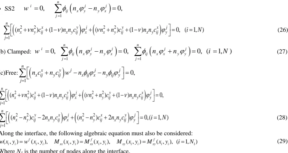
(28)Along the interface, the following algebraic equation must also be considered:
1
( , )i i f( , ),i i xx( , )i i xxf( , ),i i xy( , )i i xyf( , ), (i i 1, )
w x y w x y M x y M x y M x y M x y i N
(29) Where N1 is the number of nodes along the interface.
4. NUMERICAL RESULTS
For the present results, Gaussian weight function with a circular influence domain is adopted for the MLS approximation because of its partial derivatives with respect to x and y coordinates exist to any desired order. It takes the form of [16-18]:
2 2
2
exp( (
/ ) )
exp( ( / ) )
( )
1 exp( ( / ) )
0
ii i
i
d
c
r c
d
r
w x
r c
d
r
(30)
Where
d
i
(
x
x
i)
2
(
y
y
i)
2 , is the distance from a nodal xi to a field x in the influence domain of xi. r is theradius of support domain and c is the dilation parameter In the present work, the dilation parameter is selected such as: c=r/4.
Also, a scaling factor dmax is defined as: max m
r
d
g
(31)Where gm is the grid size, which can be regarded as the distance between the nodal point xi and the 2 nd
nearest neighboring field nodes. For regular FD grid spaced by hm, gm can be taken as: gm= .
For practical purposes the numerical results are normalized such as [18]: For squared plates:
4 2
100 s/ ( ), ij 10 ij / ( ), ij ij / , ( , , ).
w wD qa M M qa
E i jx y(32) For skew rhombic plate shown in Fig. (3):
4 2
1600 s / ( ), ij 40 ij / ( ), ij ij / , ( , , ).
w wD qa M M qa
E i jx y(33) Where
w M
,
ij,
ijare the normalized deflection, moments, and stresses, respectively. a is a composite width, (a= a1+a2).s
D
is the flexural rigidity of the isotropic plate.A numerical scheme is designed to investigate the influence of computational characteristics,( radius of support domain r, completeness order of the basis functions Nc, and scaling factors dmax ) on accuracy of the obtained results. The boundary conditions (25-29) are directly substituted into equilibrium ones (21). The reduced system is
a
θ x
y
b
solved using MATLAB. The problem is solved over a regular grid with N1= (7, 9,.., 25). For the concerned boundary conditions, Table (1) shows that the results for N1 = 11 are nearly the same as those corresponding to N1= (13,15,..,25). Therefore, a grid 11X11 nodes is considered to implement the parametric study. For different scaling factors dmax (ranging from 2 to 10) and completeness order Nc, (ranging from 2 to 7), accurate results can be attained when dmax
≤
Nc + 0.5, as in Figs. (4) and (5). This was previously recorded in [17].Table I
Comparison between the obtained deflection and the previous analytical ones at the centre of a squared plate: Nc=5, dmax=8.
Boundary conditions Number
of grid nodes
SS1 SS2 CC
Exact [4, 29] Obtained results Exact [4, 29] Obtained results Exact [4, 29] Obtained results
7x7 0.4273 0.1094 0.4273 0.7236 0.1496 0.1691
9x9 0.4273 0.2858 0.4273 0.4204 0.1496 0.1534
11x11 0.4273 0.42708 0.4273 0.427311 0.1496 0.1505
13x13 0.4273 0.427295 0.4273 0.4273 0.1496 0.1510
15x15 0.4273 0.4273 0.4273 0.4273 0.1496 0.1507
9 10 11 12 13 14 15
Number of grid points N1
Nc=2 0.6 0.7 0.8 0.9 1.0 N o rm al iz ed c en te r d ef le ct io n Present results h=1.5 Previous results[36] Isotropic (2,18) (12,16) (0,0) (16,14) x y Present results h=0.5 dmax=6 dmax=7 dmax=8 dmax=6 dmax=7 dmax=8
9 10 11 12 13 14 15
Number of grid points N1
Nc=3 0.2 0.3 0.4 0.5 0.6 0.7 0.8 0.9 1.0 N o rm a li z ed c en te r d ef le ct io n Present results h=1.5 Previous results[36] Isotropic (2,18) (12,16) (0,0) (16,14) x y Present results h=0.5 dmax=6 dmax=7 dmax=8 dmax=6 dmax=7 dmax=8
9 10 11 12 13 14 15
Number of grid points N1
Nc=4 0.900 0.925 0.950 0.975 1.000 1.025 1.050 N o rm a li z ed c en te r d ef le ct io n Present results h=1.5 Previous results[36] Isotropic (2,18) (12,16) (0,0) (16,14) x
y Present results
h=0.5 dmax=6 dmax=7 dmax=8 dmax=6 dmax=7 dmax=8
9 10 11 12 13 14 15
Number of grid points N1
Nc=5 1.00 1.25 1.50 1.75 2.00 2.25 2.50 N o rm al iz ed c en te r d ef le ct io n Present results h=1.5 Previous results[36] Isotropic (2,18) (12,16) (0,0) (16,14) x y Present results h=0.5 dmax=6 dmax=7 dmax=8 dmax=6 dmax=7 dmax=8
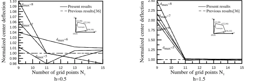
Fig. 4. Variation of the results with the completeness order Nc , scaling factor dmax and the number of grid points N1 for an irregular quadrilateral
plate with various thickness h.
9 10 11 12 13 14 15
Number of grid points N1
h=0.5 0.98 0.99 1.00 1.01 1.02 1.03 1.04 1.05 1.06 1.07 1.08 1.09 1.10 N o rm al iz ed c en te r d ef le ct io n Present results Previous results[36] Isotropic (2,18) (12,16) (0,0) (16,14) x y dmax=6 dmax=5 dmax=7 dmax=8
9 10 11 12 13 14 15
Number of grid points N1
h=1.5 1.00 1.25 1.50 1.75 2.00 2.25 2.50 N o rm al iz ed c en te r d ef le ct io n Present results Previous results[36] Isotropic (2,18) (12,16) (0,0) (16,14) x y dmax=6 dmax=5 dmax=7 dmax=8
Fig. 5. Variation of the results with the scaling factor dmax and the number of grid points N1 for an irregular quadrilateral plate with
To examine the validity of the obtained results, the bending problem of regular and irregular isotropic plates is solved and compared with the previous analytical ones in [4, 29, 34, and 35]. Tables (2) to (5) show a very good agreement between the obtained results and the previous analytical solutions. For simply supported plates, the error between obtained results and the previous exact ones in [4, 29, 34, and 35] is . While this error is
for clamped plates. Figures (4) and (5), show also that the accuracy of the obtained results increases with
increasing both of the completeness order Nc and the radius of support domain r for different values of plate thickness h. These results exactly agrees with that recorded in[36].
Table II
Comparison between the obtained deflection and the previous analytical ones [4, 29] for clamped circular plate at the centre.
Table III
Comparison between the obtained deflection and the previous analytical ones for clamped rectangular plates at the centre.
Support
size
Exact [4, 29]
Obtained results
N
c=4
N
c=5
N
c=6
N
c=7
r=.7a
1.6339
1.6339
1.3924
1.5590
3.0671
r=.8a
1.6339
1.6339
1.6339
1.6339
1.6501
r=.9a
1.6339
1.6339
1.6339
1.6339
1.6288
r=a
1.6339
1.6339
1.6339
1.6339
1.6339
r=1.1a
1.6339
1.6339
1.6339
1.6339
1.6339
b/a
W(0,0) 1 1.1 1.2 1.3 1.4 1.5 1.6 1.7 1.8 1.9 2
Exact
[4,29] 0.00126 0.00150 0.00172 0.00191 0.00207 0.00220 0.00230 0.00238 0.00245 0.00249 0.00254
Obtained
Table IV
Comparison between the obtained deflection and the previous analytical ones [4, 29] for simply supported square plates.
Table V
Comparison between the obtained deflection and the previous analytical ones [34, 35] for simply supported skew rhombic plates at the centre.
x y
.5- -.4 -.3 .2- .1- 0 .1 .2 .3 .4 .5
Exact[4,29] Obtained results Exact[4,29] Obtained results Exact[4,29] Obtained results Exact[4,29] Obtained results Exact[4,29] Obtained results Exact[4,29] Obtained results Exact[4,29] Obtained results Exact[4,29] Obtained results Exact[4,29] Obtained results Exact[4,29] Obtained results Exact[4,29] Obtained results
-.5 0 0 0 0 0 0 0 0 0 0 0 0 0 0 0 0 0 0 0 0 0 0
-.4 0 0 .040691 .0406914 .076366 .076365 .103675 .10367497 .12069 .1206897 .126456 .1264556 .12069 .1206897 .103675 .10367497 .076366 .076365 .040691 .0406914 0 0 -.3 0 0 .078388 .0783882 .146964 .1469640 .199333 .1993326 .231903 .2319025 .24293 .2429299 .231903 .2319025 .199333 .1993326 .146964 .1469640 .078388 .0783882 0 0 -.2 0 0 .109917 .1099169 .205700 .2057002 .278562 .2785617 .32376 .3237596 .339044 .3390438 .32376 .3237596 .278562 .2785617 .205700 .2057002 .109917 .1099169 0 0 -.1 0 0 .131702 .13170197 .245875 .2458755 .33235 .3323497 .385855 .3858547 .403936 .403928 .385855 .3858547 .33235 .3323497 .245875 .2458755 .131702 .13170197 0 0 0 0 0 .139800 .1398003 .260577 .2605766 .351854 .3518542 .408268 .4082679 .427314 .42731396 .408268 .4082679 .351854 .3518542 .260577 .2605766 .139800 .1398003 0 0 .1 0 0 .131702 .13170197 .245875 .2458755 .33235 .3323497 .385855 .3858547 .403936 .403928 .385855 .3858547 .33235 .3323497 .245875 .2458755 .131702 .13170197 0 0 .2 0 0 .109917 .1099169 .205700 .2057002 .278562 .2785617 .32376 .3237596 .339044 .3390438 .32376 .3237596 .278562 .2785617 .205700 .2057002 .109917 .1099169 0 0 .3 0 0 .078388 .0783882 .146964 .1469640 .199333 .1993326 .231903 .2319025 .24293 .2429299 .231903 .2319025 .199333 .1993326 .146964 .1469640 .078388 .0783882 0 0 .4 0 0 .040691 .0406914 .076366 .076365 .103675 .10367497 .12069 .1206897 .126456 .1264556 .12069 .1206897 .103675 .10367497 .076366 .076365 .040691 .0406914 0 0
.5 0 0 0 0 0 0 0 0 0 0 0 0 0 0 0 0 0 0 0 0 0 0
θ
Support size
150 300 450 600 750
Exact Obtained results Exact Obtained results Exact Obtained results Exact Obtained results Exact Obtained results
[34] [35] Nc=4 Nc=5 [34] [35] Nc=4 Nc=5 [34] [35] Nc=4 Nc=5 [34] [35] Nc=4 Nc=5 [34] [35] Nc=4 Nc=5
r=.5a .0640 .0605 0.0651 0.0626 .6609 .6587 0.6429 0.6248 2.1193 2.1285 1.4257 1.7483 4.1026 4.1079 0.7151 1.2063 5.8231 5.8172 1.574 3.4005
r=.6a .0640 .0605 0.0641 0.0651 .6609 .6587 0.651 0.6466 2.1193 2.1285 1.9384 1.9394 4.1026 4.1079 3.0779 3.1346 5.8231 5.8172 4.7888 5.1277
r=.7a .0640 .0605 0.0632 0.0647 .6609 .6587 0.655 0.6452 2.1193 2.1285 2.0541 2.0109 4.1026 4.1079 3.8776 3.7838 5.8231 5.8172 5.5824 5.6014
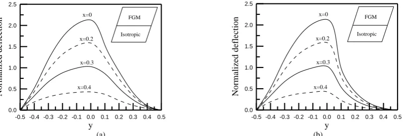
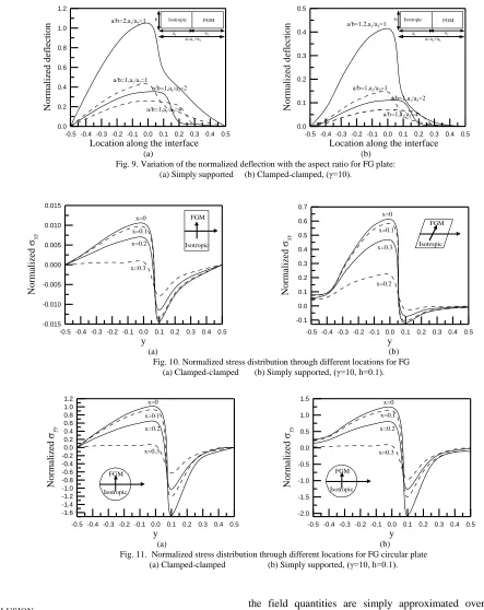
Further, a parametric study is introduced to investigate the effect of geometric and elastic characteristics of the plate on behavior of the obtained results. Figures (6-9) show that the values of normalized deflection decrease with increasing both of the graduation parameter γ and the interface location (a1/a2). While, these values increase with
increasing of the aspect ratio (a/b), as shown in Figs. (9), where a and b are the width and length of the rectangular plate. Figures (10) and (11) show normalized stress distribution, yy , through different locations of the composite.
Figures (6-11) insist the advantage of FG composites treating the material discontinuity problems.
-0.5 -0.4 -0.3 -0.2 -0.1 0.0 0.1 0.2 0.3 0.4 0.5
y 0.00
0.04 0.08 0.12 0.16
N
o
rm
al
iz
ed
d
ef
le
ct
io
n
Isotropic FGM x=0
x=0.2
x=0.3
x=0.4
-0.5 -0.4 -0.3 -0.2 -0.1 0.0 0.1 0.2 0.3 0.4 0.5
y 0.00
0.04 0.08 0.12 0.16
N
o
rm
al
iz
ed
d
ef
le
ct
io
n
Isotropic FGM
x=0
x=0.2
x=0.3
x=0.4
(a) (b)
Fig. 6. Normalized deflection distribution through different locations for FG clamped rectangular plate: (a) γ=1 (b) γ=10
-0.5 -0.4 -0.3 -0.2 -0.1 0.0 0.1 0.2 0.3 0.4 0.5
y 0.0
0.5 1.0 1.5 2.0 2.5
N
o
rm
al
iz
ed
d
ef
le
ct
io
n x=0
x=0.2
x=0.3
x=0.4
FGM Isotropic
-0.5 -0.4 -0.3 -0.2 -0.1 0.0 0.1 0.2 0.3 0.4 0.5
y 0.0
0.5 1.0 1.5 2.0 2.5
N
o
rm
al
iz
ed
d
ef
le
ct
io
n x=0
x=0.2
x=0.3
x=0.4
FGM Isotropic
(a) (b)
Fig. 7. Normalized deflection distribution through different locations for FG simply supported skew plate: (a) γ=1 (b) γ=10
-0.5 -0.4 -0.3 -0.2 -0.1 0.0 0.1 0.2 0.3 0.4 0.5
y 0
1 2 3 4 5 6 7 8
N
o
rm
al
iz
ed
d
ef
le
ct
io
n x=0
x=0.2
x=0.3
x=0.4
FGM Isotropic
-0.5 -0.4 -0.3 -0.2 -0.1 0.0 0.1 0.2 0.3 0.4 0.5
y 0
1 2 3 4 5 6 7 8
N
o
rm
al
iz
ed
d
ef
le
ct
io
n x=0
x=0.2
x=0.3
x=0.4
FGM Isotropic
(a) (b)
5. CONCLUSION
This work extends the applications of quadrature techniques for solving bending problems of regular and irregular FG composites. The method of solution consists of MLSDQM and FDM. This overcame the computational difficulties arising with the application of MLSDQ approximations. The shape function and their partial derivatives are simply determined. As well as, derivatives of
the field quantities are simply approximated over a finite difference grid. The obtained results agreed with the previous analytical and numerical ones. Further a parametric study is introduced to investigate the effects of computational, geometric, and elastic characteristics of the problem on values of the obtained results.
-0.5 -0.4 -0.3 -0.2 -0.1 0.0 0.1 0.2 0.3 0.4 0.5
Location along the interface 0.0
0.2 0.4 0.6 0.8 1.0 1.2
N
o
rm
al
iz
ed
d
ef
le
ct
io
n FGM
a1 a2
b
a=a1+a2
a/b=2,a1/a2=1
a/b=1,a1/a2=2
a/b=1,a1/a2=4
a/b=1,a1/a2=1
Isotropic
-0.5 -0.4 -0.3 -0.2 -0.1 0.0 0.1 0.2 0.3 0.4 0.5
Location along the interface 0.0
0.1 0.2 0.3 0.4 0.5
N
o
rm
al
iz
ed
d
ef
le
ct
io
n Isotropic FGM
a1 a2
b
a=a1+a2
a/b=1.2,a1/a2=1
a/b=1,a1/a2=2
a/b=1,a1/a2=4
a/b=1,a1/a2=1
(a) (b) Fig. 9. Variation of the normalized deflection with the aspect ratio for FG plate:
(a) Simply supported (b) Clamped-clamped, (γ=10).
-0.5 -0.4 -0.3 -0.2 -0.1 0.0 0.1 0.2 0.3 0.4 0.5
y -0.015
-0.010 -0.005 0.000 0.005 0.010 0.015
N
o
rm
al
iz
ed
yy
x=0 x=0.1 x=0.2
x=0.3
FGM
Isotropic
-0.5 -0.4 -0.3 -0.2 -0.1 0.0 0.1 0.2 0.3 0.4 0.5
y -0.1
0.0 0.1 0.2 0.3 0.4 0.5 0.6 0.7
N
o
rm
al
iz
ed
yy
x=0 x=0.1
x=0.2 x=0.3
FGM
Isotropic
(a) (b) Fig. 10. Normalized stress distribution through different locations for FG
(a) Clamped-clamped (b) Simply supported, (γ=10, h=0.1).
-0.5 -0.4 -0.3 -0.2 -0.1 0.0 0.1 0.2 0.3 0.4 0.5
y -1.6
-1.4 -1.2 -1.0 -0.8 -0.6 -0.4 -0.2 0.0 0.2 0.4 0.6 0.8 1.0 1.2
N
o
rm
al
iz
ed
yy
x=0 x=0.1 x=0.2
x=0.3
FGM Isotropic
-0.5 -0.4 -0.3 -0.2 -0.1 0.0 0.1 0.2 0.3 0.4 0.5
y -2.0
-1.5 -1.0 -0.5 0.0 0.5 1.0 1.5
N
o
rm
al
iz
ed
yy
x=0 x=0.1 x=0.2
x=0.3 FGM
Isotropic
(a) (b)
Fig. 11. Normalized stress distribution through different locations for FG circular plate (a) Clamped-clamped (b) Simply supported, (γ=10, h=0.1).
REFERENCES
[1] Ichikawa K., editor, Functionally graded materials in the 21st Century: a work shop on trends and forecasts, Japan. Kluwer Academic Publishers, (2000).
[2] Wang C.M., Lim G.T., Reddy J.N., Lee K.H.;'' Relationships between bending solutions of Reissner and Mindlin plate theories'', Eng. Struct.,23: 838–849, (2001).
[3] Ashraf M. Zenkour;'' Exact mixed-classical solutions for the bending analysis of shear deformable rectangular plates'', Appl. Math. Model, 27: 515–534, (2003).
[4] Timoshenko S.P., Woinowsky-Krieger S., Theory of plates and shells, 2nd Edition, McGraw-Hill, New York, (1959).
[5] Tran Minh Tu , Le Ngoc Thach, Tran Huu Quoc ; ''Finite element modeling for bending and vibration analysis of laminated and sandwich composite plates based on higher-order theory'', Computational Materials Science ,49: S390–S394,(2010).
[6] Hrabok M.M., Hrudey T.M.;" A review and catalogue of plate bending finite elements ", Computers & Structures,19: 479-495,(1984).
[7] Liew K.M., Wang C.M., Xiang Y., Kitipornchai S., Vibration of Mindlin Plates—Programming the p-Version Ritz Method, Elsevier Science, Oxford, (1998).
[8] Gupta U.S., Jain S.K., Jain D.;'' Method of collocation by derivatives in the study of axisymmetric vibration of circular plates'', Computers and Structures, 57: 841–845, (1995).
[9] Masa. Tanaka, Matsumoto T., Shiozaki A.;" Application of the
boundary-domain-element method to the harmonic-bending-vibration problem of thin elastic plates ", Engineering Analysis with Boundary Elements ,13: 239-247,(1994).
[10] Masa. Tanaka, Bercin A.N.;"Static bending analysis of stiffened plates using the boundary element method ", Engineering Analysis with Boundary Elements, 21: 147-154, (1998).
[11] Civalek Ö;"Three-dimensional vibration, buckling and bending analyses of thick rectangular plates based on discrete singular convolution method ", International Journal of Mechanical Sciences, 49: 752-765, (2007).
[12] Civalek Ö;" A four-node discrete singular convolution for geometric transformation and its application to numerical solution of vibration problem of arbitrary straight-sided quadrilateral plates ", Applied Mathematical Modelling, 33: 300-314, (2009).
[13] Belytschko T., Krongauz Y., Organ D., Fleming M., Krysl P.;'' Meshless methods: an overview and recent developments'', Computer Methods in Applied Mechanics and Engineering ,139: 3–47, (1996). [14] Jafari A.A., Eftekhari S.A.; " An efficient mixed methodology for
free vibration and buckling analysis of orthotropic rectangular plates" , Applied Mathematics and Computation, 218: 2670-2692, (2011). [15] Xinwei Wang, Zhe Wu; " Differential quadrature analysis of free
vibration of rhombic plates with free edges", Applied Mathematics and Computation, 225: 171-183, (2013).
[16] Liew K.M., Huang Y.Q., Reddy J.N.; '' A hybrid moving least squares and differential quadrature (MLSDQ) meshfree method'', Int.J. Comput. Engrg. Sci. , 3: 1–12, (2002) .
[17] Liew K.M., Huang Y.Q., Reddy J.N.; "Analysis of general shaped thin plates by the moving least squares differential quadrature method", Finite Elements in Analysis and Design, 40: 1453-1474, (2004).
[18] Liew K. M., Haung Y. Q., Reddy J. N.; "Moving least squares differential quadrature method and its application to the analysis of shear deformable plates", Int. J. Numer. Meth. Engng. , 56: 2331-2351, (2003).
[19] Liew K.M., Xin Zhao, Ferreira A.J.M; " A review of meshless methods for laminated and functionally graded plates and shells", Composite Structures, 93:2031-2041, (2011).
[20] Ping Zhu, Zhang L.W., Liew K.M.;" Geometrically nonlinear thermo mechanical analysis of moderately thick functionally graded plates using a local Petrov-Galerkin approach with moving Kriging interpolation", Composite Structures, 107:298-314, (2014).
[21] Lanhe W., Hongjun W, Daobin W.; '' Dynamic stability analysis of FGM plates by the moving least squares differential quadrature method'', Composite Structures, 77:383-394, (2007).
[22] Zhang L.W., Zhu P., Liew K.M.;" Thermal buckling of functionally graded plates using a local Kriging meshless method", Composite Structures, 108:472-492, (2014).
[23] Bui T.Q., Nguyen M.N., Zhang Ch.; "Buckling analysis of Reissner-Mindlin plates subjected to in plane edge loads using a shear locking free and mesh free method ", Engineering Analysis with Boundary Elements , 35: 1038-1053, (2011).
[24] Ola Ragb, Matbuly M.S., Nassar M.; " Analysis of Composite Plates Using Moving Least Squares Differential Quadrature Method", Applied Mathematics and Computation, 238: 225–236, (2014). [25] Wen P.H.,Ali abadi M.H.,'' A hybrid finite difference and moving
least square method for elasticity problems'', Engineering Analysis with Boundary Elements, 36: 600–605,(2012).
[26] Jensen P.S.,''Finite difference technique for variable grids'', Comput Struct ,2:17–29, (1972).
[27] Liszka T.,Orkisz j.,''The finite difference method at arbitrary irregular grids and its application in applied mechanics'', Comput Struct, 11:83–95,( 1980).
[28] Panc. V., Theory of elastic plates, Leydon : Noordhoff International Publishing, 13-41, (1975).
[29] Reddy J.N., Theory and analysis of elastic plates, Taylor& Francis: Philadelphia, PA, (1999).
[30] Reddy J.N., Mechanics of laminated composite plates. Theory and Analysis, CRC Press, Boca Raton, Fl, (1997).
[31] Lancaster P., Salkauskas K.; "Surfaces generated by moving least squares methods", Mathematics of computation, 37: 141-158, (1981).
[32] Breitkopf P., Rassineux A., Touzot G., Villon P.; ''Explicit form and efficient computation of MLS shape functions and their derivatives'', Int. J. Numer. Methods Engrg. 48: 451–466, (2000).
[33] Belytschko T., Krongauz Y., Fleming M., Organ D., Liu W.K.; " Smoothing and accelerated computations in the element free Galerkin method", Journal of Computational and Applied Mathematics ,74: 111-126, (1996).
[34] Liew K. M., Han J. B.;"Bending analysis of simply supported shear deformable skew plates", Journal of Engineering Mechanics (ASCE), 123: 214-221, (1997).
[35] Sengupta D.; "Performance study of a simple finite element in the analysis of skew rhombic plates ", Computers and Structures, 54:1173-1182, (1995).

![Table IV Comparison between the obtained deflection and the previous analytical ones [4, 29] for simply supported square plates](https://thumb-us.123doks.com/thumbv2/123dok_us/1362777.1645600/9.842.44.801.98.324/table-comparison-obtained-deflection-previous-analytical-simply-supported.webp)