e-ISSN: 2278-7461, p-ISSN: 2319-6491
Volume 5, Issue 4 [March 2016] PP: 07-12
A Declared Concept and a Proposed Algorithm to Assess HRV for
Heart Disease Diagnosis
Mazhar B. Tayel
1and Eslam I AlSaba
21, 2 Electrical Engineering Department, Faculty of Engineering. Alexandria University, Alexandria, Egypt.
Abstract: Nowadays, Variability of Heart Rate (HRV) becomes utmost important tool for predicting and
diagnosing most of diseases. It depends on the diversity of heart complex wave. As heart complex wave is non-linear wave, therefore HRV is stochastic and chaotic (stochaotic) signal. HRV needs a very sensitive tool for analysing and predicting its variability. In previous era, Rosenstein (R) and Wolf (W) had used the Lyapunov exponent (LE) as a quantitative measure for HRV detection sensitivity, but the Rosenstein and Wolf methods diverge in determining the main features of HRV sensitivity, while Mazhar-Eslam introduce a modified algorithm to overcome the Rosenstein and Wolf drawbacks. Mazhar-Eslam Variability Frequency (MVF) used as quantitative and qualitative measure for HRV detection sensitivity.
The present work introduces a novel reliable method to analyze the linear and nonlinear behaviour of heart complex wave variability, and to assess the use of the HRV as a versatile tool for heart disease diagnosis. This paper introduces a declaration for the concept of the LE parameters to be used for HRV diagnosis and proposes a modified algorithm for a more sensitive parameters computation.
Keywords: Lyapunov exponent (LE), stochaotic, Heart Rate Variability (HRV), Variability Frequency
I.
INTRODUCTION
Variability of the Heart Rate (HRV) act as a universal measurement which used for analyzing heart activity. All actions and reactions effect and affect by the heart. Therefore, HRV analysis indicates reflection on the body status. Different pattern can describe the fluctuations in HR such as (linear, non-linear pattern), which classified into periodical and aperiodical oscillation. These patterns can be quantified in time domain using statistical analysis, in order to estimation the RR- fluctuations intervals.
The spectrum of HRV analysis shows HR band frequency variations. Which classified into three pattern: High, low and very low frequency band which vary from (0.15-0.5) Hz, (0.05-0.14) Hz, and (0.01-0.04) respectively. The higher band represent vagal modulation fragment indicator, and the lowerst one indicates an overwhelmingly sympathetic tone and baroreflex activity [1, 2, 3]. There are many research studied the linearity of HRV [4], But, it failed in full quantification the dynamic structure of the HR signals in order to extraction a highly sensitive diagnostic method for HR diseases.
In this work we introduces an insight about the most reliable method to analyze the linear and nonlinear behaviour of heart complex wave variability, Also assess the use of the HRV as a versatile measurement for heart disease diagnosis. This novelty introduces new algorithm called Mazhar-Eslam algorithm which considering whole cases of linear and nonlinear behaviour of the HRV signal and pattern.
II.
DECLARATION
OF
PARAMETERS
Careful study of equation (1) identifies that the definition of Λ in [10, 11] as an exponent is far from fact, since it has dimension of time reciprocal, i.e. it represents some sort of repetition frequency in periodic and aperiodic signals. Also, in the case of chaotic attractors, it represents variations among the attractors.
(1)
Considering the physiological, psychological, and environmental stochastic-chaotic (stochaotic) nature of variability in HRs, the mentioned above repetition frequency must be defined as variability frequency (VF) in HRs, which is to be expressed as
(Hz) (2)
MVF ( ) for almost all SED initial conditions in a bounded dynamical system is to be used as a definition of deterministic stochaotic.
Take a case of two identical simple harmonic oscillators with different amplitudes. Because the frequency is independent of amplitude, a phase portrait of the two oscillators would be a pair of concentric circles. The orbits in this situation would maintain a constant separation. Finally, a positive MVF ( > 0) implies the orbits are on a stochaotic attractor.Nearby points, no matter how close, will diverge to any arbitrary separation. These points are unstable [7].
A negativeMVF means that the orbit attracts to a stable fixed point or stable periodic orbit. Negative MVFs are characteristic of dissipative or non-conservative systems. Such systems exhibit asymptotic stability. The more negative the MVF, the greater the stability. Super stable fixed points and super stable periodic points have a MVF tends to infinity ( → − ∞). This is something similar to a critically damped oscillator in that the system heads towards its equilibrium point as quickly as possible.
Also, a zero MVF means that the orbit is a neutral fixed point (or an eventually fixed point). An MVF of zero value indicates that the system is in some sort of steady state mode. A physical system with zero MVF is conservative. Such systems exhibit stability.
III.
DISCUSSION
The introduced MVF " " divergence of initially SED nearby trajectories in state-space is coupled with folding of trajectories. To discriminate between stochaotic dynamics, periodic, and aperiodic signals, the MVF " s" are often to be used as a qualitative measure of SED. The trajectories of stochaotic signals in state-space follow typical patterns. Closely state-spaced trajectories converge and diverge exponentially, relative to each other. Therefore, the existence of a positive MVF for almost all initial conditions in a bounded dynamical system is to be used for the deterministic stochaotic HRV cases.
Table 1 shows the spectrum bands of the normal HRV and some cases from MIT-BIH database, using the three algorithms: Mazhar-Eslam, Wolf, and Rosenstein, used to compare the SED precision of the three algorithms in determining the MVF.
It is worth to note that the introduced Mazhar-Eslam algorithm spectral analysis of the given HRV reveals three distinct frequency bands in the modulation of humans HRs. The first band is very low frequency (VLF) band in the range (0.01-0.05 Hz), the second band is low frequency (LF) band in the range (0.06 -0.15 Hz) and the third band is a high frequency (HF) band in the range (0.16-0.50 Hz) as illustrated in (Fig 2). These results coincides with that mentioned in [8].
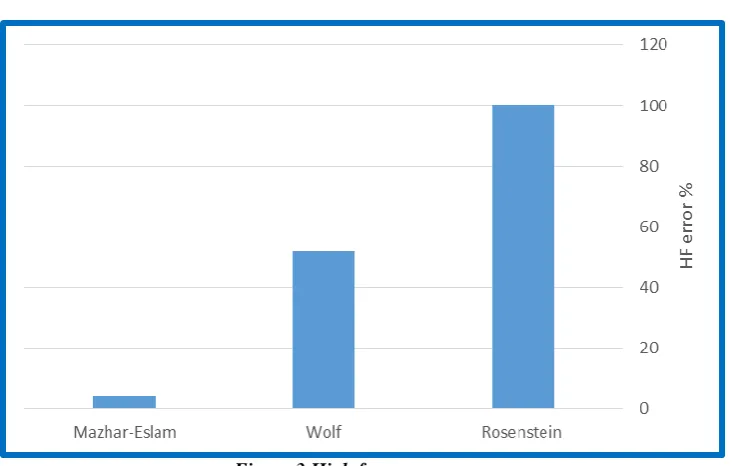
Figure 2 The introduced MVF spectrum bands of HRVs. The new measure is high frequency error is calculated as
(3)
Therefore, the high frequency error rH for MVF algorithms shown in table (1) are Rosenstein
Wolf
Mazhar-Eslam
Table 1 The MVF results of different methods using normal case and MIT-BIH sample cases.
Parameter MVF
Seria
l Method
Case
Rosenstein Wolf Mazhar-Eslam
1 Normal 0.7586 (HF) 0.505 (HF) 0.4986 (HF)
2 101 0.2500 (HF) 0.1700 (HF) 0.0830 (LF)
3 102 0.1600 (HF) 0.1300 (LF) 0.0530 (VLF)
4 104 0.2100 (HF) 0.1300 (LF) 0.0700 (LF)
5 106 0.2300 (HF) 0.1500 (LF) 0.0770 (LF)
6 107 0.2000 (HF) 0.1300 (LF) 0.0667 (LF)
7 109 0.2200 (HF) 0.1400 (LF) 0.0733 (LF)
8 111 0.2400 (HF) 0.1600 (HF) 0.0800 (LF)
9 112 0.2400 (HF) 0.1700 (HF) 0.0800 (LF)
10 115 0.2800 (HF) 0.1700 (HF) 0.0930 (LF)
11 117 0.2300 (HF) 0.1600 (HF) 0.0770 (LF)
12 118 0.2500 (HF) 0.1600 (HF) 0.0833 (LF)
13 119 0.2700 (HF) 0.1700 (HF) 0.0900 (LF)
14 121 0.2500 (HF) 0.1600 (HF) 0.0840 (LF)
15 122 0.2300 (HF) 0.1600 (HF) 0.0770 (LF)
16 123 0.2300 (HF) 0.1500 (LF) 0.0770 (LF)
17 124 0.2500 (HF) 0.1700 (HF) 0.0840 (LF)
18 200 0.2300 (HF) 0.1500 (LF) 0.0770 (LF)
19 203 0.2300 (HF) 0.1500 (LF) 0.0770 (LF)
20 212 0.2100 (HF) 0.1400 (LF) 0.0700 (LF)
21 221 0.2100 (HF) 0.1400 (LF) 0.0700 (LF)
22 230 0.2100 (HF) 0.1400 (LF) 0.0700 (LF)
23 231 0.2200 (HF) 0.1500 (LF) 0.0740 (LF)
* HF high frequency, LF low frequency, and VLF very low frequency.
Figure 3 High frequency error.
is low. Table 1 shows that the Mazhar-Eslam algorithm for MVF is more precise than Wolf and Rosenstein algorithms. Also, the Mazhar-Eslam algorithm shows that the selected cases from MIT-BIH are in the low frequency range as its spectrum variation indicate ( Hz). The Wolf algorithm has less precision than Mazhar-Eslam algorithm. Wolf observed incorrect band for cases 111, 112, 115, 117, 118, 119, 121, 122, 124, and 231 because they are not in the high frequency band as it shows but they are in the low frequency band as mentioned before. The worst and imprecise algorithm is Rosenstein as it shows all cases in the high frequency band. Thus, the Mazhar-Eslam is a recommended algorithm for HRV analysis.
Figure 4 The MVF diagnosis diagram for ventricular and supraventricular
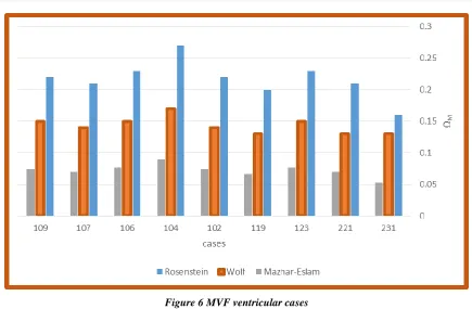
Figure 6 MVF ventricular cases
IV.
CONCLUSION
Heart Rate Variability (HRV) is reported in several cardiological and non-cardiological diseases. Also, it has a prognostic value and is therefore very important in modelling the cardiac risk. HRV is stochaotic signal that remains highly controversial. In order to have utmost importance, HRV needs a sensitive measure to analyse it. It is concluded that Mazhar-Eslam variability mean frequency (MVF), is a versatile and more precise qualitative SD measure of HRV sensitivity than others. The Rosenstein algorithm provided less sensitive estimates than the Wolf algorithm to capture differences in local dynamic stability from small gait data sets. The data supported the idea that this latter outcome results from the ability and inability of the Wolf algorithm and Rosenstein algorithm, respectively, to estimate adequately MVF of attractors with an important rate of convergence as those in gait. Therefore, the Mazhar-Eslam algorithm appears to be more qualitative and appropriate to evaluate local dynamic stability from small gait data (SD) sets like HRV. Increase in the size of data set has been shown to make the results of the Mazhar-Eslam algorithm more suitable, although other means as increasing the sample size might have a similar effect. The Mazhar-Eslam algorithm uses the merits of the Discrete Wavelet Transform (DWT) instead of Fats Fourier Transform (FFT) unlike Rosenstein and Wolf. The Mazhar-Eslam algorithm cares for all SD variants especially the small ones like that are in HRV. These SD variants may contain many important data to diagnose diseases as R-R interval has many SD variants. Thus, the Mazhar-Eslam algorithm for MVF ( ) taking determination all of s is characterized by its high SD robust nest, and precise qualitative predictor. The Mazhar-Eslam algorithm presents a new chapter for HRV diseases diagnosis. It contains a positive part for HRV as it is stochaotic signal.
.
REFERENCES
[1]. A.E. Aubert and D. Ramaekers. Neurocardiology: the benefits of irregularity. The basics of methodology, physiology and current clinical applications. ActaCardiologica, 54(3):107–120, 1999.
[2]. Akselrod S, Gordon D, Ubel FA, Shannon DC, Barger AC, Cohen R. Power spectral analysis of heart rate fluctuations: a quantitative probe of beat-to-beat cardiovascular control. Science 1981;213:220-222. [3]. Mortara A, La Rovere MT, Pinna GD, Prpa A, Maestri R, Febo O, Pozzollo M, Opasich C, Tavazzi L.
Arterial baroreflex modulation of heart rate in chronic heart failure. Circulation 1997;96(10):3450-3458. [4]. Hartikainen JEK, Tahvanainen KUO, Kuusela TA. Shortterm measurement of heart rate variability, p.
149-176, In: Clinical guide to cardiac autonomic tests, M Malik ed., Kluwer Ac Publ, Dordrecht 1998. [5]. Backs, R. W. (1998). A comparison of factor analytic methods of obtaining cardiovascular autonomic
components for the assessment of mental work load. [heart rate analysis]. Ergonomics. 41, 733-745. [6]. Mazhar B. Tayel and Eslam I AlSaba. Robust and Sensitive Method of Lyapunov Exponent for Heart
[7]. U.R. Acharya, K.P. Joseph, N. Kannathal, C.M Lim, and J.S. Suri. Heart rate variability: a review. Medical and Biological Engineering and Computing, 44(12):1031–1051, 2006.
[8]. V. Moga, C. Ioana, I. Bonchis, Florina Parv, T. Ciocarlie, C. Tudoran, Mariana Moga, Rodica Avram. The clinical value of nonlinear dynamics parameters in the assessment of the arrhythmic risk. Journal of Experimental Medical & Surgical Research, Cercetãri Experimentale & Medico Chirurgicale Year XVIII · Nr.3/2011 · Pag. 107 – 112
[9]. ROSENSTEIN, M. T., COLLINS, J. J., AND DE LUCA, C. J. A practical method for calculating largest lyapunov exponents from small data sets. Phys. D 65, 1-2 (1993), 117–134.
[10]. WOLF, A., SWIFT, J., SWINNEY, H., AND VASTANO, J. Determining lyapunov exponents from a time series Physica D: Nonlinear Phenomena 16, 3 (July 1985), 285–317.