Income and Wealth in
The Irish Longitudinal
Study on Ageing
VINCENT O’SULLIVAN Lancaster University
BRIAN NOLAN Oxford University
ALAN BARRETT
Economic and Social Research Institute, Dublin Trinity College Dublin
CARA DOOLEY Trinity College Dublin
Abstract: Between 2009 and 2011, data were collected under the first wave of The Irish Longitudinal Study on Ageing(TILDA). Over 8,500 people aged 50 and over and living in Ireland were interviewed about a wide range of topics covering socio-economic and health issues. Our primary goals in this paper are to present details on two of the variables which will be of particular interest to economists, namely income and wealth, and to discuss issues in relation to their use. We describe how the income and wealth data were collected. We assess the quality of the income data by comparing them to those obtained through the European Union Survey on Income and Living Conditions(EU-SILC). We examine the joint distribution of income and assets and conduct a small exercise on using the data to design a means-testing system.
329
I INTRODUCTION
B
etween late 2009 and early 2011, fieldwork was conducted on Wave 1 of The Irish Longitudinal Study on Ageing, TILDA. The fieldwork involved the collection of data on a nationally-representative sample of over 8,500 people aged 50 and over and living in Ireland. The data were collected through three routes – a computer-assisted personal interview (CAPI), a self-completed questionnaire (SCQ) and an extensive health assessment (HA). Through TILDA, Ireland has joined a growing international trend through which the issues associated with an ageing population are studied in part through a longitudinal study of the older population.Given that data are collected through three routes, the amount of data which is available for each individual in the sample is large and covers a wide range of topics. The CAPI questionnaire was used to collect information on a full range of socio-demographic issues, including topics such as education, labour force status, income and wealth. Questions were also asked about family structure, migration history, health status (mental and physical), retirement planning and healthcare utilisation. The SCQ covered more sensitive topics such as alcohol consumption, quality of relationships and childhood traumas including physical and sexual abuse. Finally, the health assessments were used to collect objective information on the health status of each individual and included tests related to cardiovascular health, optical health, cognition and gait and balance. The existence of this new data, and its augmentation through the collection of subsequent waves, opens up a range of important research opportunities across a range of disciplines.
In this paper, our first objective is to present details on two of the variables which will be of particular interest to economists, namely income and wealth. While income is collected in the EU Survey of Income and Living Conditions (EU-SILC), wealth data at the individual or household level has not been collected in Ireland since the late 1980s. This makes the TILDA wealth data rare within Ireland. More broadly, as the TILDA data also contain huge amounts of information on health status and life satisfaction, the potential to use the data to analyse the links between economic circumstances and health and well-being is enormous.
sources and by exploring whether the TILDA data produces reasonable measures of quantities such as Gini coefficients. Our aim in this section is partly to inform other researchers in Ireland, and elsewhere, of the existence and quality of the income and wealth data.
In Section III, we move onto an exploration of the joint distribution of income and wealth. One reason for our interest in the joint distribution arises from the issue of means testing. As the removal of universal entitlements for older people is increasingly discussed, the question arises of how to implement means testing taking account of both income and wealth. We use the data to illustrate some implications of using certain income and wealth thresholds in determining eligibility for entitlements. In Section IV, we conclude.
II DATA DESCRIPTION
2.1 Collection of Income Data
Before describing how income and wealth data were collected in TILDA, it is important to outline one key feature of how the sample was generated. As no population register exists in Ireland, it was necessary to call on houses to establish if there was a person aged 50 or older resident. If there was, this household was eligible and all people aged 50 or over in the household were interviewed (where possible), along with spouses or partners aged under 50. In this way, the TILDA sample includes multiple people from the same households and this is relevant to generating data on household income.
During the TILDA CAPI interview, all respondents were asked a series of questions about their sources of income covering income from employment, social welfare, pensions, investment incomes and other sources. The questions were taken directly from the recent versions of the European Union Survey on Income and Living Conditions(EU-SILC) questionnaire. EU-SILC is a pan-European survey conducted annually in most EU countries which collects extremely detailed information about different sources of income and also a limited number of demographic variables such as household structure and education levels. By using the same questions as in EU-SILC, it is possible to compare the data that is generated and we exploit this below.
non-response problem is far less severe. However, and as discussed at greater length below, using the single comprehensive household income question seriously under-estimates disposable household income when compared with external data.
The alternative approach to the single comprehensive household income question is to aggregate, within each household, every source of individual level gross income. The final amount of household disposable income is then calculated by aggregating gross income from all sources across all of the individuals in the household and then estimating income net of tax and social insurance contributions. The different sources of gross income are: employee income, self-employment income, pension income (from both private and occupational schemes), investment income, rental income as well as income from all social welfare schemes in operation in Ireland.
The Irish tax system is not fully individualised so in order to calculate net household income it is crucial to have income information on both partners in the case of couples. Other information pertinent to the tax system was also used in the calculation of household income net of tax and social insurance contributions. For example, TILDA collects detailed information on pension contributions which are tax deductible. Furthermore, household structure, housing tenure type and employment type enabled us to assign the appropriate tax credits. For example, PAYE workers receive a tax credit in contrast to self-employed people.
For both approaches to measuring household income, a final equivalised household disposable income was created to account for differences in household size. Equivalisation takes economies of scale in consumption into account when describing the per person standard of living within a household. Different equivalisation weighting schemes are used internationally. Here we used the scheme most often used in Ireland which assigns a weight of 1 to the head of household, 0.66 to all subsequent household members aged fourteen or older and 0.33 to those aged younger than fourteen years.1
2.2 Collection of Wealth Data
Wealth is collected in a much more straightforward manner than income. To shorten the interview and under the assumption that wealth is pooled within the household, the wealth questions were asked only to a nominated “financial respondent” who declares that they are the best informed member
1While this approach to equivalisation makes intuitive sense when thinking about households
of the household on matters relating to wealth. In slightly over 60 per cent of households with two respondents the financial respondent is the male partner.
Initially, the financial respondent is asked if they or their partner hold certain types of assets. The assets are: owner-occupied residential property; savings on deposits; financial assets; cars; non owner-occupied housing and other types of assets such as a business or land. Flash cards are used so that respondents are sure as to what to include. They are then asked to put values on different categories of assets that they or their partner own. Questions relating to debt are also asked and the distinction between mortgage and non-mortgage debt is made so information on both types of debt is collected.
As the data were mostly collected during 2010, a time of continued house-price declines in Ireland, a question arises over the accuracy of the house house-price data. Daft.ie (a major property web-site in Ireland) reported that the average asking price across the country in 2010 was €220,000. We find an average value of €287,000. As the TILDA respondents were more likely to be living in mature areas, the average value is not implausible. However, it should be noted that the possibility exists of actual prices in 2010 being below the asking prices reported by Daft and so uncertainty remains over the accuracy of the house-price data.
A major problem with income and particularly wealth data is the level of non-response. To reduce non-response to the income and wealth questions the technique of “unfolding brackets” was used. Those who refused or claimed not to know the relevant amount in relation to an income or wealth question were asked a follow-up question which gave the option of providing a banded answer rather than a point estimate. Table 1 shows that the use of unfolding brackets was a relatively successful interview strategy as the non-response was reduced significantly, especially in relation to housing wealth.2Generally, the results presented in this paper use the mid-points of the unfolding brackets as the inputted data points for those who did not answer the original questions. An alternative approach to the use of mid-points of brackets is to randomly draw values within brackets. The advantage of this approach is that, unlike the mid-point approach, it does not assume away within-bracket inequality and so does not impart a downward bias to measured inequality.3
2An error in the questionnaire omitted the unfolding bracket in relation to savings on deposit.
This results in a much higher rate of missing cases for this item than would have otherwise been. The mistake has been rectified for Wave 2.
3Researchers wanting to examine socio-economic inequalities in health using the TILDA data
We point out the impact of moving from one approach to the other when discussing Gini coefficients below.
Finally, income from assets has been inferred by applying a rate of interest to relevant wealth stocks when interest earned is unknown. As only 4 per cent of total gross income is income from assets (based on an assumed interest rate of 5 per cent), the sensitivity of total gross income to the interest rate assumption is limited. For example, if we assumed a 1 per cent interest rate as opposed to a 5 per cent rate, mean net disposable household income falls by about 1 per cent.
Extending the idea of using incomplete/partial information further, there are a number of other imputation options open to the researcher who wishes to reduce the occurrence of missing values. Cameron and Trevedi (2005) provide an introduction to imputation methods such as single and multiple imputation. One should be aware that these techniques often rely on un-testable and, in the case of income and wealth, perhaps questionable assumptions that the missing values are occurring at random and are unrelated to the true value of the observation.
Table 1: Missing Cases for Income and Asset Questions
Proportion Proportion of Missing of Missing
Cases Cases Without Using Using
Unfolding Unfolding Brackets Brackets*
Employee Income 0.11 0.04
Self-employment Profit or Loss, Directors’ Fees 0.38 0.24 Asset Income from Interest, Dividends, Rent & Other 0.36 0.16
Farm Income 0.17 0.08
Income From Private or Occupational Pensions 0.15 0.15 Social Benefits/Allowances 0.06 0.06
Catch-All Question on Total Net Household Income 0.24 0.07
Housing 0.28 0.06
Savings 0.30 0.23
Financial Assets 0.19 0.09
Cars 0.13 0.13
Property 0.05 0.05
Other Assets 0.10 0.06
We experimented with multiple imputation, with a view to providing a sense of the difference between the estimated mean income and wealth levels when imputation is and is not used. The variables used to impute were: region; marital status; number of children; household size; home ownership; age (of both spouses where applicable); economic status (of both spouses where applicable) and education (of both spouses where applicable). We carried out the imputation using STATA 12’s mi impute command which fills in missing values of a continuous variable using the Gaussian normal regression imputation method. We report on the results below.
Finally it is worth noting that the income and wealth questions are located towards the end of the CAPI interview. There is a concern that respondents may be less willing to discuss this topic, which for some is sensitive, at the end of a very lengthy interview. However, the feedback from focus groups of respondents and interviewers is that by the end of the interview the interviewer has built up a rapport with the respondents and that sensitive topics are more easily discussed.
2.3 Defining the Sample for the Analyses Presented Below
In order to assess the quality of the data (relative to EU-SILC), and so that we can undertake some applications of the data, we need to define the specific sub-sample which will be used. Although we use multiple imputation for illustrative purposes, we generally want to restrict the analyses to cases where we have no missing data so we need to explore which measure of household income to use. As mentioned above, the single comprehensive household income question has a far lower rate of missing observations than when using the aggregated sources of gross income approach as the latter approach is highly data intensive. Using the single comprehensive household income question results in a sample of 5,342 that is very similar in its demographic characteristics to the original sample (see the first and last column of Table 2). However, as we shall see in the next section, the single comprehensive household income question tends to underestimate household disposable income.
of whom are 50 years old or older, are living together. Calculating their tax bill is problematic and would involve making assumptions that could not be tested.
Second, not all respondents answered the individually-based financial information questions in the survey be they in relation to income or wealth.
Table 2: Characteristics of Groups Omitted/Included in Final Sample
Original Partner Missing Contra- Missing Final Final Sample Did Income dictory Asset Sample Sample
Not Informa- Answers Data Using Using
Respond* tion Aggregate Single
Sources of Compre-Income hensive Income Level of Education:
Primary 0.38 0.36 0.33 0.15 0.43 0.42 0.38 Secondary 0.43 0.45 0.41 0.54 0.41 0.43 0.44 Third 0.19 0.19 0.26 0.30 0.16 0.15 0.18 Age Group:
50-64 0.58 0.65 0.54 0.95 0.51 0.56 0.59 65-74 0.23 0.21 0.26 0.05 0.24 0.25 0.24 >=75 0.18 0.14 0.20 0.00 0.25 0.19 0.18 Gender:
Male 0.48 0.43 0.52 0.62 0.46 0.48 0.50 Female 0.52 0.57 0.48 0.38 0.54 0.52 0.50 Location:
Dublin 0.22 0.23 0.23 0.19 0.18 0.24 0.24 Urban outside
of Dublin 0.28 0.29 0.29 0.22 0.31 0.27 0.27 Rural 0.49 0.49 0.48 0.59 0.51 0.48 0.49 Marital Status:
Married 0.68 1.00 0.72 0.84 0.60 0.56 0.65 Single 0.10 0.00 0.09 0.08 0.11 0.12 0.11 Divorced/
Seperated/
Widow(er) 0.22 0.00 0.19 0.08 0.30 0.32 0.24 No. of Children Present:
No Children 0.52 0.07 0.65 0.43 0.66 0.67 0.55 One Child 0.24 0.48 0.18 0.21 0.18 0.18 0.23 Two Children 0.12 0.21 0.10 0.17 0.09 0.09 0.12 Three or More
Children 0.11 0.24 0.07 0.19 0.07 0.07 0.10
_n 8,504 1,812 1,284 408 1,399 3,601 5,342
Third, in a small number of cases, clearly implausible answers were given and so these observations are not used in our analysis. These were mostly people who claimed to be making pension contributions in excess of their income. Given that pension contributions are taken into account when calculating disposable income we felt it appropriate to drop these observations.4
Despite the large number of lost observations, one can see from the first column and second last columns of Table 2 that the final sample from the aggregated sources of income approach closely resembles the nationally representative original TILDA sample when looking at the distribution of key demographic variables such as education, age group, geographic location and gender. However, in relation to household structure there are some differences as our sample under-represents married couples due to the lack of full information on household finances within some married couples.
No detailed income information was collected in relation to household members other than those aged 50 or over and their spouses. The final row of Table 2 shows that children are present in one-third of households in the sample. The majority of these children were in education or unemployed – 60 per cent. For the unemployed, we assumed that their income was the maximum value of job seekers’ allowance. The remaining 40 per cent were working so we needed to find a reasonable proxy for their incomes. From EU-SILC, and looking specifically at people under the age of 50 who are living with their parents, we found that university graduates were earning €496 per week and that non-university graduates were earning €355 per week. We assumed that these were the earnings of the children in the TILDA sample, depending on their graduate status.5
2.4 External Validity of the Income Data
From Table 3 one can see that the medians and means of equivalised weekly household income from the TILDA and EU-SILC samples appear similar when we use the aggregated sources of gross income approach. One should note that the EU-SILC sample used here is a sub-sample with the same inclusion criteria as the TILDA sample – households with at least one person aged 50 or over. Figure 1 shows the distribution of disposable income from TILDA (Aggregated Sources of Gross Income) and EU-SILC again appear to be closely aligned.
In order to test if the appearance of similarity holds in statistical terms, we ran a Kolmogorov-Smirnov test and this rejected the null that the
4However when the analysis was repeated using these observations, the results were found to be
roughly the same.
Table 3: Comparison of Mean and Median Income in TILDA and Similarly Defined Sample in EU-SILC
Mean Median
TILDA TILDA EU-SILC TILDA TILDA EU-SILC Single Aggregated Single Aggregated
Compre- Sources Compre- Sources
hensive of hensive of
Income Income Income Income
Question Question
Total Net Disposable 644 740 819 480 553 623 Household Income
After Social Transfers Using National Definition of Income
(Standard Error) (17) (20) (19) (8) (9) (14)
Equivalised Income 357 428 423 267 316 342 After Social Transfers
Using National Definition of Income and National Equivalence Scale
(Standard Error) (9) (11) (7) (2) (5) (6)
n = 4,041 for EU-SILC 2010.
distributions are the same. Given this, researchers should be conscious of how the TILDA distribution differs from that of EU-SILC to assess if the differences have any substantive impacts on results or conclusions. The points at which the distributions differ can be seen in Figure 1.
The TILDA values in Table 3 are based on cases without missing data. We noted above that we experimented with multiple imputation and the results suggested that significant differences arise depending on which approach is used. As Table 3 shows, if cases with missing data are excluded, mean total net disposable household income is estimated to be €740. This figure rises to €792 when multiple imputation is used. In the case of equivalised income, the difference is negligible – €430 with multiple imputation compared to €428 without.
with a 95 per cent C.I. of 0.122 to 0.153) from the same period.6Being at risk of poverty is defined as being below 60 per cent of the median of the income distribution. In 2010 this was €10,831 per annum (= €208 per week). One should note that, at the time of the survey, non-age related social welfare payments were set at around €196 per week whereas the higher rates of age-related social welfare were set above the poverty threshold (e.g., the full rate of Non-Contributory Pension was €219 per week).
Taking another perspective, the Gini Coefficient for equivalised household income from EU-SILC 2010 for a similarly defined sample was 0.326 (with a 95 per cent C.I. of 0.312 to 0.341) which is very similar to the Gini Coefficient estimated using TILDA (0.347 with a 95 per cent C.I. of 0.331 to 0.363). When we use random draws as opposed to midpoints for the unfolding brackets, the Gini coefficient rises to 0.35. Putting the Irish Gini Coefficient into international perspective, the Gini Coefficient for Sweden in 2010 was 0.23, the EU average was 0.304 in 2010 and the corresponding number for the USA was 0.47 in 2009. In the case of each of these comparators, it should be noted that the Gini is calculated for all age groups and not just those aged over 50 which is the case with our calculations for TILDA.
Figure 1: The Distribution of Weekly Equivalised Household Disposable Income
0.4
0.35
0.3
0.25
0.2
0.15
0.1
0.05
0
EU-SILC
TILDA
0–200
301–400 501–600 701–800901–1,0001,101–1,2001,301–1,4001,501–1,6001,701–1,8001,901–2,000
6Although similar, a test for the equality of the estimated poverty rates rejected the null with a
We find that the single comprehensive household income approach underestimates household disposable income more so than the aggregate sources of gross income approach. Using this measure of income the estimated at risk of poverty rate is 26 per cent and the Gini coefficient is around 0.42.7 These numbers do not compare favourably with a similarly defined sample from the EU-SILC data. For the observations where both the single comprehensive income question and the aggregated sources of income are recorded, the correlation between these two measures of income is just 0.16. One cannot reject the null of independence between these two measures of income when estimating Spearman’s Rank Correlation Coefficient. Therefore, one must question the validity of the single comprehensive income question despite the larger sample size that it provides. In Wave 2 of TILDA, collected in late 2012, the respondents were asked the comprehensive income question in relation to each household member separately so as to try to reduce the likelihood that the income of some family members is not included in total household income.
For the remainder of the paper, the measure of income used is the aggregate sources of gross income approach. However, the results are qualitatively similar when using the single comprehensive question approach. For others using the TILDA income data, they key point to be taken from the analysis here is as follows. Although the distribution of income under the aggregated sources approach in TILDA looks similar to the corresponding distribution based on EU-SILC, the formal statistical testing of equality does not confirm that they are statistically the same. The Kolmogorov-Smirnov tests are quite demanding and it may well be that in specific circumstances, the differences between the TILDA and EU-SILC distributions may have minimal impacts on research findings. However, there is an onus on researchers to establish this with reference to their research questions.
2.5 External Validity of the Wealth Data
Relative to the widespread availability of income data, it is rare for wealth data to be collected and even rarer for both wealth and income data to be collected in a large sample. Not since 1987 has detailed wealth data been collected on such a large sample in Ireland. We classify the asset holdings of the TILDA respondents into two categories: non-liquid assets and liquid assets. Table 4 shows the percentage of respondents holding different types of assets and the average self-assessed value of these assets.
7The increase in the Gini coefficient as we move between the two measures of income suggests
Non-liquid assets consist of owner-occupied housing, non-owner occupied housing and other fixed assets which include land, a firm or business, an inheritance or money owed to the respondent. The level of home ownership is 85 per cent which is high relative to other countries. According to Census 2011, around 70 per cent of all Irish households own their dwelling outright or are paying off a mortgage.
Liquid assets are savings in deposit accounts, financial assets (current cash value of life insurance, mutual funds, bonds or shares) and cars. The level of ownership of financial assets at 28 per cent is low compared to the US. Of TILDA respondents 79 per cent say they own at least one car although 9 per cent give a value of zero to the car. This is very similar to the Census 2006 figure which showed that 80 per cent of Irish households owned at least one car.
TILDA also collected information about levels of debt. Debt is classified as mortgage debt on owner occupied housing or other types of debt such as credit card debt. The number of people in debt is low and the amounts owed are generally low. It can be shown that the position of households in the relative wealth distribution does not vary much if one examines the net asset distribution or the gross asset distribution. In spite of this, a Kolmogorov-Smirnov test rejects the null that the gross and net distributions are the same.
Table 4: Descriptive Statistics Relating to Assets and Debt
Proportion With Mean of Standard Type of Asset/Debt Non-Zero Error
Observations
Owner Occupied Housing 0.85 287,151 14,104 Other Property 0.11 275,210 21,580 Other Fixed Assets 0.17 187,975 18,520 Total Non-Liquid Assets 0.87 351,001 15,876
Savings 0.64 62,796 6,616
Financial Assets 0.28 66,656 7,814
Cars 0.79 7,814 291
Total Liquid Assets 0.81 76,954 6,780
Debt 0.25 32,994 3,789
Mortgage Debt 0.13 75,478 6,734 Total Debt 0.30 55,888 4,461
For this reason, the same “health warning” should be made here that was made in respect of income above. Researchers should be conscious of the statistical difference between the gross and net distributions and should assess whether this matters substantively in the context of their research question.
The Gini Coefficient in relation to gross wealth is 0.529 which is much greater than when looking at inequality in relation to income. As was the case when looking at income, the Gini Cofficient rises (to 0.55) when random values within unfolding brackets are used instead of mid-points.8 The higher Gini with respect to wealth compared to income would be expected as wealth measures the accumulation of resources over the lifetime of the individual and inequality tends to accumulate over time. It is more difficult to provide international context for the estimated wealth Gini Coefficient as there are very few surveys which record wealth (and even fewer that record both income and wealth). The last available estimate for Ireland was 0.581 in 1987. The UK had a wealth Gini Coefficient of 0.697 in 2000, Sweden’s was 0.742 in 2002 and the USA’s was 0.801 in 2001. The ranking of wealth inequality by country can differ greatly relative to the same country’s ranking in relation to income inequality. This is due to the level of home ownership and other incentives to accumulate wealth in a given economy. Ireland’s level of wealth inequality is low when compared internationally and this may reflect the high level of home ownership amongst the TILDA sample.
The use of multiple imputation has a significant impact on our estimate of average wealth. Using complete cases, and including observations who reported zero wealth, we estimate average gross wealth to be €362,345; our estimate when wealth is imputed for missing values is €387,386. This mirrors the effect which the use of multiple imputation had on one of the income measures and so indicates that thought should be given to whether complete-case samples or imputation should be used.
III THE JOINT DISTRIBUTION OF INCOME AND WEALTH AND MEANS TESTING
These data hold out great potential for analysis of the joint distribution of income and wealth and its implications across various domains. This is most timely given the context of austerity and the longer-run issue of population ageing. The TILDA data allow us to see the extent to which elderly people on high incomes are also those with high levels of wealth, and whether those on
8The Gini for net wealth when random values within unfolding brackets are used instead of
low incomes for the most part have little or no wealth. This is highly relevant to a rounded assessment of the economic circumstances of the elderly and to inequalities amongst them, and to the framing and assessment of tax and transfer policies and reforms.
Table 5 shows the joint distribution of wealth and income. Around 37 per cent of people are in the bottom two quartiles of both distributions. Around 28 per cent are in the top two quartiles of the two distributions. Around 17 per cent are in the top two quartiles of the income distribution but in the bottom two quartiles of the wealth distribution. Similarly, around 17 per cent are in the top half of the income distribution but in the bottom half of the wealth distribution.
Table 5: Joint Distribution of Equivalised Income and Gross Assets
Equivalised Equivalised Equivalised Equivalised
Income Income Income Income
Quartile 1 Quartile 2 Quartile 3 Quartile 4 Gross Asset Quartile 1 0.12 0.09 0.05 0.02 Gross Asset Quartile 2 0.08 0.08 0.07 0.03 Gross Asset Quartile 3 0.05 0.07 0.06 0.06 Gross Asset Quartile 4 0.02 0.03 0.06 0.10
The upper panel of Table 6 shows the proportion of those holding different types of assets across different quintiles of income. Home ownership is near ubiquitous in the top three quintiles. Ownership of second homes is concentrated in the upper two quintiles. The proportion of those with other assets (including land and business assets) rises across the quintiles. One should note that the bottom income quintile includes self-employed people who have made a loss (coded to zero income). As there are only 21 such people, this will make little difference to the overall calculations. Car ownership amongst the top two quintiles of income is very high compared to the bottom three quintiles. The proportion of those with savings increases across the quintiles. However, holdings of financial assets are much higher in the top two quintiles than in the bottom two quintiles. Mortgage debt is higher amongst those with higher incomes. This mortgage debt relates to the principal residence so the greater debt of those with higher incomes is not related to the second homes owned by this group. Rather the greater level of debt may reflect the fact that those in the top income quintiles are those who are still receiving full salaries rather than pensions and are thus younger and still repaying mortgages.
the bottom three quintiles, and to a lesser extent the 4th quintile, is broadly similar. Around three-quarters of their gross wealth is held as housing. However, in the top quintile, less than two thirds of wealth is held as housing and a larger proportion held as savings.
The bottom panel of Table 6 shows the median asset holdings of different types of assets across the income distribution. Median levels of housing wealth rise in a roughly linear fashion across the quintiles. However, business assets, savings and financial assets are much larger for those in the top two quintiles than those in the bottom three quintiles.
Focusing towards the bottom of the income and wealth distribution, these data also allow us to examine the joint distribution of income poverty and what one might term ‘wealth poverty’. We showed already that almost 16 per cent of the sample is at risk of income poverty based on the poverty line being set at 60 per cent of median incomes (where the median income is taken from EU-SILC). In order to get a corresponding estimate of wealth poverty, we have to rely on the TILDA data itself due to the absence of an alternative source of wealth data. If we include all zero responses and use the gross wealth measure, then 60 per cent of median gross wealth is €147,000 and we use this as our wealth poverty line.
Table 6: Characteristics of Wealth by Income Quintiles
Owner Other Busi- Cars Savings Finan- Mort- Other Occupied Housing ness on cial gage Debt
Housing Assets Deposit Assets Debt Proportion Holding Asset
Income Quintile 1 0.77 0.03 0.13 0.59 0.47 0.16 0.06 0.20 Income Quintile 2 0.82 0.04 0.17 0.61 0.59 0.16 0.05 0.16 Income Quintile 3 0.89 0.08 0.15 0.78 0.67 0.25 0.14 0.25 Income Quintile 4 0.92 0.16 0.19 0.84 0.77 0.34 0.14 0.32 Income Quintile 5 0.95 0.26 0.22 0.89 0.87 0.48 0.17 0.28
Proportion of Total Gross Asset Portfolio
Income Quintile 1 0.75 0.02 0.04 0.06 0.10 0.03 0.04 0.06 Income Quintile 2 0.74 0.02 0.07 0.05 0.11 0.02 0.02 5.44 Income Quintile 3 0.74 0.03 0.06 0.04 0.09 0.04 0.03 0.04 Income Quintile 4 0.70 0.06 0.06 0.03 0.10 0.05 0.09 0.04 Income Quintile 5 0.62 0.07 0.07 0.02 0.15 0.06 0.03 0.04
Median Holding of Asset
Turning to Table 7, it can be seen that of the 16 per cent who are income poor, over half are not ‘wealth poor’. In targeting social transfers and other supports, a means test based solely on income would thus direct resources towards substantial numbers of households with wealth above 60 per cent of median wealth. In practice, wealth as well as income is often taken into account in determining eligibility for such programmes – in the Irish case this applies to both social assistance pensions and entitlement to free health care, for example.9 However, analysis of the distributional incidence of such programmes and of possible reforms is most often based on income only, driven by the absence of data on wealth. The TILDA data thus open up new avenues for analysis of means testing where both wealth and income are included.
Table 7: The Joint Distribution of Income Poverty and Wealth Poverty
Wealth Not Poor Wealth Poor
Income Not Poor 0.62 0.22
Income Poor 0.09 0.07
In Table 8, we illustrate this in terms of the following scenario – the government aims to provide a benefit to the 10 per cent least well-off older households, and some combination of wealth and income means testing is to be employed to identify eligible households. By employing an income test only, almost 16 per cent of households would be eligible and this leaves too many households eligible. This is the first line in Table 8 and corresponds to the sum of the bottom two cells in Table 7. By imposing a (relatively high) wealth test
9For the non-contributory old age pension, for example, savings, investments, cash on hand and
any property owned (other than one’s own home) are assessed as capital with a formula applied to derive the weekly means from such capital.
Table 8: Means Test of Wealth Using Threshold Based on Proportion of Median Gross Assets
Proportion Who are Poor
No Wealth Means Test 0.157
Twice Median Gross Assets 0.144 1.5 times Median Gross Assets 0.128
Median Gross Assets 0.106
of twice median wealth, the government takes the wealthiest households out of the eligible group, even though these households are income poor. This still leaves over 14.4 per cent of older households in the eligible group. This exceeds the 10 per cent target and so the wealth test must be made more stringent. It can be seen from Table 8 that a wealth test which imposes a cut-off at median gross assets leaves the eligible group just above the 10 per cent target. If the 60 per cent of median approach had been taken with respect to wealth, identical to the approach taken with income, only 7 per cent of households would have been eligible (this is the bottom-right cell in Table 7). In this case, the chances of “false negatives” would have risen, in the sense that more low income households would have been excluded than was needed under the 10 per cent target.
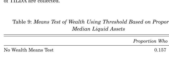
A potential argument against wealth-based means testing is that non-liquid assets may be of limited use in funding day-to-day living expenses and so should be excluded. Such exclusions occur in practice, for example, in the case of medical cards. In Table 9, we repeat the scenario of Table 8 but now we have excluded property, business and other fixed assets and focus just on savings and financial assets. Table 9 shows that the liquid wealth cut-off would need to be around half of median liquid assets to achieve the 10 per cent target.
Of course, the inclusion and treatment of income and wealth in means-tests generates a host of incentive effects which can work against other objectives of policy (see Sefton et al, 2008 and Sefton and van de Ven, 2009). However, the data provide the potential to tease out the impact of different combinations of means tests in a static setting, with the possibility of investigating behavioural responses to future policy changes as further waves of TILDA are collected.
Table 9: Means Test of Wealth Using Threshold Based on Proportion of Median Liquid Assets
Proportion Who are Poor
No Wealth Means Test 0.157
Twice Median Liquid Assets 0.126 1.5 times Median Liquid Assets 0.121
Median Liquid Assets 0.114
IV CONCLUSIONS
Our main objective in this paper has been to introduce researchers to both the existence, and potential usefulness, of the income and wealth data in TILDA. In presenting the data, we have drawn attention to some of the complex issues which arise due to the presence of missing data. This is a problem which afflicts all surveys, especially relating to financial issues. We have shown how different approaches to the data, such as the use of multiple imputation and the treatment of unfolding brackets, can impact upon the data and how care should be taken in deciding what approach to adopt in analyses. While the TILDA income data, in particular based on aggregating sources from the survey, match the EU-SILC data quite well, the matching is not perfect based on formal statistical testing. Researchers should be aware of this and should explore whether the statistical differences between the TILDA and EU-SILC distributions matter in a substantive way in the context of the research questions being addressed.
The data hold out great potential, in particular for analysis of the joint distribution of income and wealth and its implications across various domains. Here we have illustrated this by focusing towards the bottom of the distributions and examining the proportions of households falling below various income and wealth cut-offs. The richness of the TILDA data would also allow for the characteristics of the individuals and households involved to be investigated in some depth.
More generally, the TILDA data are unusually strong, even in an international context, in combining both health and socio-economic data. The health data are both subjective and objective and cover both physical and mental health. Such rich health data, when combined with the data on income and wealth, provide researchers with an opportunity to develop research which seeks to relate economic and health outcomes (see Smith, 2007).
REFERENCES
CAMERON, A.C. and P. TRIVEDI, 2005. Microeconometrics. Methods and Applica -tions,New York: Cambridge University Press.
CLARKE, P. and T. VANOURTI. 2010. “Calculating the Concentration Index when Income is Grouped”, Journal of Health Economics, Vol. 29, pp. 151-157.
SEFTON, J., J. VAN DE VEN, 2009. “Optimal Design of Means-Tested Retirement Benefits”, Economic Journal,Vol. 119, pp. F461-F481.