A SOLUTION FOR THE BI-OBJECTIVE VEHICLE ROUTING
PROBLEM WITH TIME WINDOWS USING LOCAL SEARCH
AND GENETIC ALGORITHMS
Anan Mungwattana1, Tharinee Manisri2, Kanjanaporn Charoenpol3, Gerrit K. Janssens4
1 Kasetsart University, Bangkok, Thailand 2 Sripatum University, Bangkok, Thailand 3 Surindra Rajabhat University, Surin, Thailand 4 Hasselt University, Diepenbeek, Belgium
Received 22 June 2015; accepted 6 May 2016
Abstract: This paper deals with the vehicle routing problem with time windows (VRPTW). The VRPTW routes a set of vehicles to service customers having two-sided time windows, i.e. earliest and latest start of service times. The demand requests are served by capacitated vehicles with limited travel times to return to the depot. The purpose of this paper is to develop a hybrid algorithm that uses the modified push forward insertion heuristic (MPFIH), a λ-interchange local search descent method (λ-LSD) and a genetic algorithm to solve the VRPTW with two objectives. The first objective aims to determine the minimum number of vehicles required and the second is to find the solution that minimizes the total travel time. A set of well-known benchmark problems are used to compare the quality of solutions. The results show that the proposed algorithm provides effective solutions compared with best found solutions and better than another heuristic used for comparison.
Keywords:vehicle routing problem with time windows (VRPTW), genetic algorithms, local search.
4 Corresponding author: [email protected]
1. Introduction
The vehicle routing problem (VRP) belongs to the class of NP-hard combinatorial problems which require a substantial amount of time to determine optimal solutions for large problems. The fundamental objectives are to determine the minimum number of vehicles, the minimal travel time or the minimal costs of the travelled routes. However, in real world applications, the VRP is extended by constraints such as vehicle capacity or time interval in which
within an earliest and latest start of service time of the customer without exceeding the route time of the vehicle and exceeding the vehicle capacity. The route time of a vehicle is defined as the sum of the waiting times, the service times and the travel times. A vehicle that reaches a customer before the earliest start of service time, after the latest start of service time and after the maximum route time incurs waiting time, tardiness time and overtime, respectively. Finally, the total customer demand in each route cannot exceed the capacity of the vehicle.
The rest of this paper is organized as follows. Section 2 reviews relevant VRPTWs and algorithms to solve them. Section 3 presents the methodology to solve the problem under study. Section 4 presents and discusses the results. Finally, conclusions and future work opportunities are added in section 5.
2. Literature Review
The VRPTW is a well-known and complex combinatorial problem with considerable economic significance (Christofides, 1985). The VRPTW is more complex than the Travelling Salesman Problem (TSP) as it considers servicing customers with time windows using multiple vehicles. Savelsbergh (1985) has shown that finding a feasible solution to the Traveling Salesman Problem with time windows (TSPTW) is an NP-complete problem (see also Braekers et al. (2014) for full truckload applications). Although, optimal solutions to the VRPTW can be obtained using exact methods, the computational time required to solve a VRPTW optimally is prohibitive for large problems (Cordeau et al., 2002). As a result, heuristic methods are often used to obtain optimal or near optimal solution in a reasonable amount of time. Heuristic
approaches for the VRPTW use route construction, route improvement or methods that integrate both route construction and route improvement. Many researchers propose to use meta-heuristic algorithms for the VRPTW and other extensions of the VRP, called rich vehicle routing problems as introduced in Hartl et al. (2006). For example, Tarantilis et al. (2004) propose a metaheuristic for solving the heterogeneous fleet vehicle routing problem (HFFVRP). The Pickup and Delivery problem with time windows (PDPTW) has been considered by Mitrinovic-Minic and Laporte (2006). Recently, the problem in V R PT W is extended to the real-world business. The fleet size and mix vehicle routing problem with time windows (FSMVRPTW) is a specific problem of the classic vehicle routing problem. Solutions are proposed by Belfiore and Fávero (2007), Bräysy et al. (2008), Dell‘Amico et al. (2007), Dullaert et al. (2002) and Repoussis and Tarantilis (2010).
In Solomon’s paper, the time-oriented nearest neighbor insertion heuristic has shown to be very successful. Berger and Barkaoui (2004) propose a parallel version of a hybrid genetic algorithm for VRPTW. This approach is based on the simultaneous evolution of two populations of solution focusing on separate objectives subject to temporal constraint relaxation. Bräysy and Gendreau (2005a, 2005b) present a survey of the research on the VRPTW. Both traditional heuristic route construction methods and recent local search algorithms are examined in Part I. Part II gives an overview of meta-heuristic approaches for the VRPTW.
ranking technique. An advantage of this approach is that it is not necessary to derive weights for a weighted sum scoring formula. Tan et al. (2006) propose a hybrid multi-objective evolutionary algorithm (HMOEA) with specialized genetic operators and variable length chromosome representation to accommodate the sequence-oriented optimization in VRPTW. The HMOEA optimizes all routing constraints and objectives simultaneously, which improves the routing solutions in many aspects, such as lower routing cost, wider scattering area and better convergence trace. Ghoseiri and Ghannadpour (2010) develop an evolutionary algorithm for the VRPTW by incorporating various heuristics for local exploitation in the evolutionary search and the concept of Pareto’s optimality. Garcia-Najera and Bullinaria (2011) propose an improved multi-objective evolutionary algorithm for the VRPTW by adding a similarity measure between solutions. Also other conflicting objectives may be taken into account in the VRPTW. All approaches in the literature are quite effective, as they provide solutions competitive with well-known benchmark data of Solomon’s VRPTW instances (2008).
3. Methodology: Notation and Algorithm
Description
In this section the notation of the parameters of the model as well as the decision variables is explained. The model uses a fixed number of vehicles to serve a fixed number of customers from a single depot. Each customer has a known demand. The fleet of vehicles is homogeneous, i.e. they all have the same capacity. Each customer has a delivery time window, defined by an earliest and latest arrival time. The depot also has its time window. Time windows are of the soft
type, both for customers as for the depot. Late arrivals lead to a penalty per time unit of tardiness. Late arrival at the depot leads to an overtime cost.
3.1. Notation
Mathematical notations
K: number of vehicles, with index k, k = 1..K N: number of customers (including the depot), with index i, i = 1..N
Ci: customer i, with index i = 2..N C1: depot
Problem parameters
di: demand of customer i, i=2..N q: capacity of each vehicle
tij: travel time between customer i to
customer j where i, j = 1, ..., N, i ≠ j and i = 1 or j = 1 refers to the depot
ei: earliest arrival time at customer i li: latest arrival time at customer
i
bi: service time at customeri
M: maximum travel time of each vehicle
α: penalty weight factor for the waiting time
γ: penalty weight factor for the tardiness time
η: penalty weight factor for the overtime
KLB: lower bound on the number of vehicles
to be used, where
Variables
Dk: total demand for vehicle k Ai: arrival time at customer
i
wij: waiting time after departure from
customer i and before servicing customer
j, defined as wij = max[ej - (Ai + tij), 0], i, j =
2..N and i ≠ j
rik: travel time of vehicle k until customer i Wk: total waiting time for vehicle k, where k = 1..K
Ok: total overtime for vehicle k, where k
= 1..K, i.e. the time that a route served by vehicle k exceeds M
Lk: total tardiness for vehicle k, where k = 1..K Tk: total travel time for vehicle k, where k
= 1..K
Totk: total journey time for vehicle k, defined by Totk = Tk + Wk + Bk where k = 1..K
Decision variables
xijk: indicator if the customers i and j follow
each other in a route served by vehicle k (xijk
= 1) or not (xijk= 0) , where i ≠ j.
Routes
A solution to the problem is represented by a set of routes S = {R1, R2, …, RK}
Rk: route of vehicle k, i.e. a sequence of
customers served by vehicle k, where k = 1..K
Objective function
The objective function of the VRPTW is made up as a single-objective cost function. The cost function for a vehicle k consists of four parts: the travel cost, the waiting cost, the tardiness cost and the overtime cost. The cost is summed over all vehicles active in the operation:
(1)
The objective function can be written in terms of the decision variables xijk as:
where
3.2. Algorithm
The aim is to route vehicles such that the total travel time of all vehicles and their
penalties including waiting, tardiness and overtime, are minimized. Typically, the first priority aims to find the minimum number of vehicles required and the second priority aims to search for the solution that minimizes the total travel time of all vehicles (expressed as a cost) and their cost penalties with respect to waiting time, tardiness and overtime.
In this section, a two-phase algorithm for solving the VRPSTW is developed. The algorithm consists of two phases: a route construction phase and a route improvement phase. In the first phase, a modified push-forward insertion heuristic (MPFIH) is applied. The MPFIH developed by Manisri et al. (2009) is a heuristic method for inserting a customer into a route based on the push-forward insertion method. It is an efficient method for computing the insertion of a new customer into the route. The initial number of routes in this method is defined as the minimum number of vehicles necessary to satisfy total customer demand. Facing the fact that in this initial number of routes no time windows are taken into consideration, considerable penalties appear in the second, third and fourth terms of the objective function. This most probably causes an effect of significant improvement in the objective functions in the first generations. The feasibility of inserting a set of customers into route Rk is checked by inserting the
customer between all edges in the current route and selecting the edge that satisfies the vehicle capacity. The MPFIH algorithm is documented below.
Step 1: Construct two lists of customer nodes. The first list sorts the customer nodes in ascending order of ei. The second
customer i that is not allowed when creating the route and also li is the latest arrival time
in the same meaning.
Step 2: Construct two lists of customer node size KLB. The first list contains KLB elements
with the lowest values of ei. Remove the
selected customer nodes from both sets, which are created in Step 1. The second list is made up of the remaining customer nodes in descending order of li.
Step 3: Construct the matrix, Rk size KLB * 2
by the first column is Ci which the first KLB
minimum, ei and the second column is the
first KLBmaximum, li.
Step 4: Check the feasible routes, each row of matrix, Rk that satisfy the constraints. If
all rows satisfy the constraints, the initial matrix, Rk is setting by size KLB * 2.
Step 5: Remove the customer nodes from 2 sets in Step 1 that have been selected to matrix, Rk.
Step 6: Construct insertion matrix size KLB
* 1 by select the set of Ci which the next KLB
minimum, ei.
Step 7: Insert the matrix of Ci between the
column first and second column of Ci then
repeat Step 4 to Step 6 until the 2 sets of customer nodes in Step 1 are empty and all of
Ci has been inserted to routes or matrix, Rk then
the algorithm terminates. If not, go to Step 8.
Step 8: Select the remainder of each customer node, Ci which the next minimum, ei and
then insert a node to the route that has the remainder capacity.
Step 9: Remove the customer nodes that have been selected and then repeat Step 8 to Step 9.
Step 10: If all of Ci has been inserted to routes
or matrix, Rk then the algorithm terminates,
else go to Step 11.
Step 11: Construct a new route or row of matrix, Rk+i, where i = 1,...,n and then repeat
Step 9 to Step 11 until the 2 sets of customer nodes in Step 1 are empty then the algorithm terminates.
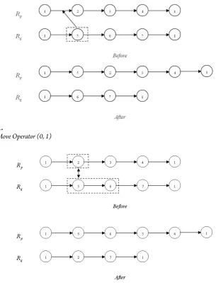
In the second phase, the route improvement algorithm applies local search and a genetic algorithm, based on the concept of iteratively improving the solution to a problem by exploring neighboring solutions. To design a λ-interchange local search descent method (λ-LSD), one typically needs to specify the following choices: how an initial feasible solution is generated; which move-generation mechanism to use; which acceptance criterion and the stopping criterion to use (Bräysy and Gendreau, 2005a). The λ-LSD searches the set of neighbors generated by the LSD for a given integer equal to 1 and 2. The move generation mechanism creates the neighboring solutions by the move operators indicated as (0, 1), (1, 0), (1, 1), (0, 2), (2, 0), (1, 2), (2, 1) and (2, 2). The operator (0, 1) on routes (Rp, Rq) indicates a shift of one
customer from route q to route p (Fig. 1). The operators (0, 1), (1, 0), (2, 0) and (0, 2) indicate a shift of one or two customers between two routes. The operators (1, 1), (1, 2), (2, 1) and (2, 2) indicate an exchange of one or two customers between two routes (Fig. 2) (Osman, 1993).
select a neighbor when implementing an improvement method: the best-improve strategy investigates the whole neighborhood
and chooses the best neighbor; the first-improve (FI) selects the first neighbor that satisfies the pre-defined acceptance criterion.
Fig. 1.
The Move Operator (0, 1)
Fig. 2.
The Move Operator (1, 2)
Then a genetic algorithm is applied to
Construct the travel time matrix using Euclidean distances; Set the penalty weight parameters which are α, γ and η;
Set the parameters for the λ-LSD and GA which are the maximum number of
iterations, the initial population size, the crossover rate (Pc) and the mutation rate (Pm);
Generate an initial population using MFPIH;
Evaluate the fitness function of the initial population members;
Repeat:
Select parent chromosome using roulette wheel selection;
Generate random numbers for the crossover and mutation operators
If random number for crossover > Pc
then
execute crossover else
execute mutation;
Evaluate fitness functions of offspring;
Increase the number of offspring in the initial solution Calculate the probabilities in choosing the chromosome.
Until the maximum number of iterations is reached
4. Results and Discussion
Typically a new algorithm is tested against well-known benchmarking problems with known characteristics. While several authors have published instances, the instances of VRP with time windows published by Solomon are the most widely used in experiments for comparison. The instances include information per customer including its location (expressed as a (x,y) coordinate), its demand, its time windows (expressed as an interval between an earliest and latest time of start of service), and a service duration. The instances are designated of the C-type, the R-type, or the RC-type. The original 56 Vehicle Routing Problems with Time Windows (VRPTW) instances designed by Solomon in 1983 contain 100 customers, but later versions are available with 25 and 50 customers. Our proposed algorithm is tested on Solomon’s VRPTW benchmarking problems including R1&R2, C1&C2 and RC1&RC2. The experiment runs on 56 VRPTW instances. All instances have 25, 50 or 100 customer nodes and a
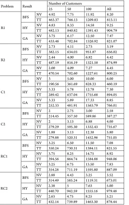
Table 1
Comparison of Results for Various Types of Problems and Different Solution Methods
Problem Result Number of Customers25 50 100 All
R1
BFS NV 4.92 7.75 11.92 8.20
TT 463.37 766.13 1209.83 813.11
HY NVTT 4.83482.13 8.33840.82 14.581391.43 904.799.25
GA NVTT 3.75433.46 6.17702.84 1326.9212.50 7.47821.07
R2
BFS NVTT 2.73382.15 4.11634.03 2.73951.87 3.19656.02
HY NVTT 2.44 487.19 4.00816.19 6.821321.58 4.42874.99
GA NV 2.00 4.09 7.27 4.45
TT 470.54 702.60 1227.61 800.25
C1
BFS NVTT 3190.56 5.00361.69 10.00828.33 6.00460.19
HY NVTT 3.33289.42 5.78637.04 12.781755.68 7.30894.05
GA NVTT 3.33252.33 5.89481.91 17.331563.79 8.85766.01
C2
BFS NV 2 2.75 3.00 2.58
TT 214.45 357.50 589.86 387.27
HY NV 2 3.13 6.88 4.00
TT 279.29 595.30 1332.43 735.67
GA NVTT 1.88279.88 3.13520.31 12.381452.96 5.80751.05
RC1
BFS NVTT 3.25350.24 6.50730.31 11.501384.11 7.08821.55
HY NVTT 3.75394.56 8.25864.74 14.751584.88 8.92948.06
GA NV 3.25 6.75 13.50 7.83
TT 354.28 711.19 1595.80 887.09
RC2
BFS NV 2.88 4.43 3.25 3.52
TT 314.49 585.24 1119.31 673.01
HY NVTT 2.38440.70 5942.59 7.631555.16 5.00979.48
GA NVTT 2.63432.14 4.75739.89 8.251463.30 5.21878.44
Table 1 illustrates the effectiveness of the results of the proposed algorithm, as it provides solutions competitive with best solutions and also provides better solutions than those obtained by Manisri et al. (2009). But there seem to be differences in the
solutions, the algorithm works mostly very good except for a few exceptions. The worst examples are found in the clustered sets C1/ C1 and RC2 with 100 customers.
5. Conclusion and Future Work
An algorithm to solve the bi-objective VRPTW has been developed using the concept of modified push forward insertion heuristic (MPFIH), a λ-interchange local search descent method (λ-LSD) and a genetic algorithm. The effectiveness of the proposed algorithm is evaluated through some of Solomon’s benchmark problem sets. The results show that the proposed algorithm, in general, provides effective solutions compared with best found solutions and better than some other heuristics.
For the future work, the cases with weak results need a closer investigation. Two questions are to be answered: (1) why do weaker results appear for the clustered sets? and (2) why do weaker results appear for the larger instances? To answer the first question, it might be useful to explore various local search strategies. No immediate advice can be formulated to answer the second question.
Acknowledgements
This work is supported by the Interuniversity Attraction Poles Programme initiated by the Belgian Science Policy Office (research project COMEX, Combinatorial Optimization: Metaheuristics & Exact Methods).
References
Belfiore, P.P.; Fávero, L.P. 2007. Scatter search for the fleet size and mix vehicle routing problem with time windows, Central European Journal of Operations Research, 15(4): 351-368.
Berger, J.; Barkaoui, M. 2004. A parallel hybrid genetic algorithm for the vehicle routing problem with time windows, Computers & Operations Research, 31(12): 2037-2053.
Bräysy, O.; Gendreau, M. 2005a. Vehicle routing problem with time windows, Part I: Route construction and local search algorithms, Transportation Science, 39(1):104-118.
Bräysy, O.; Gendreau, M. 2005b. Vehicle routing problem with time windows, Part II: Metaheuristics,
Transportation Science, 39(1): 119-139.
Bräysy, O.; Dullaert, W.; Hasle, G.; Mester, D.; Gendreau, M. 2008. An effective multirestart deterministic annealing metaheuristic for the fleet size and mix vehicle routing problem with time windows,
Transportation Science, 42(3): 371-386.
Braekers, K.; Caris, A.; Janssens, G.K. 2014. Bi-objective optimization of drayage operations in the service area of intermodal terminals, Transportation Research Part E:
Logistics and Transportation Review, 65: 50-69.
Christofides, N. 1985. Vehicle Routing. In E.L. Lawler, J.K. Lenstra, A.H.G. Rinnooy Kan, and D.B.Schmoys (eds.), The Traveling Salesman Problem: a Guided Tour
of Combinatorial Optimization, Chapter 12, Wiley,
Chichester.
Cordeau, J.-F.; Gendreau, M.; Laporte, G.; Potvin, J.-Y.; Semet, F. 2002. A guide to vehicle routing heuristics,
Journal of the Operational Research Society, 53(5): 512-522.
Dell’ Amico, M.; Monaci, M.; Pagani, C.; Vigo, D. 2007. Heuristic approaches for the fleet size and mix vehicle
routing problem with time windows, Transportation
Science, 41(4): 516-526.
Dullaert, W.; Janssens, G.K.; Sörensen, K.; Vernimmen, B. 2002. New heuristics for the fleet size and mix vehicle routing problem with time windows, Journal of
Garcia-Najera, A.; Bullinaria, J.A. 2011. An improved multi-objective evolutionary algorithm for the vehicle
routing problem with time windows, Computers &
Operations Research, 38(1): 287-300.
Ghoseiri, K.; Ghannadpour, S.F. 2010. Multi-objective vehicle routing problem with time windows using
goal programming and genetic algorithm, Applied Soft
Computing, 10(4): 1096-1107.
Hartl, R.F; Hasle, G.; Janssens, G.K. 2006. Editorial to the Special Issue on Rich Vehicle Routing Problems, Central
European Journal of Operations Research, 14(2): 103-104.
Jozefowiez, N.; Semet, F.; Talbi, E. 2008. Multi-objective vehicle routing problems, European Journal of Operational
Research, 189(2): 293-309.
Manisri, T.; Mungwattana, A.; Janssens, G.K. 2009. Algorithm for the Multi-objective Vehicle Routing
Problem with Time Windows. In Proceedings of the
5th International Congress on Logistics and Supply Chain
Management Systems, Seoul, South Korea.
Mitrinovic-Minic, S.; Laporte, G. 2006. The pickup and delivery problem with time windows and transshipment,
INFOR, 44(3): 217-227.
Ombuki, B.; Ross, B.J.; Hanshar, F. 2006. Multi-objective genetic algorithms for vehicle routing problem with time windows, Applied Intelligence, 24(1): 17-30.
Osman, I. 1993. Metastrategy simulated annealing and tabu search for the vehicle routing problem, Annals of
Operations Research, 41(4): 421-451.
Osman, I.H.; Christofides, N. 1994. Capacitated clustering problems by hybrid simulated annealing and tabu search, International Transactions in Operational
Research, 1(3): 317-336.
Repoussis, P.; Tarantilis, C. 2010. Solving the fleet size and mix vehicle routing problem with time windows via adaptive memory, Transportation Research Part C: Emerging
Technologies, 18(5): 695-712.
Savelsbergh, M.W.P. 1985. Local search for routing
problems with time windows, Annals of Operations
Research, 4(1-4): 285-305.
Solomon, M.M. 2008. VRPTW benchmark problems, Available from Internet: <http://web.cba.neu. edu/~msolomon/problems.htm>.
Tan, K.C.; Chew, Y.H.; Lee, L.H. 2006. A hybrid multiobjective evolutionary algorithm for solving vehicle
routing problem with time windows, Computational
Optimization and Applications, 34(1): 115-151.
Tarantilis, C.D.; Kiranoudis, C.T.; Vassiliadis, V.S. 2004. A threshold accepting metaheuristic for the heterogeneous fixed fleet vehicle routing problem,