Thesis by
Shriram Mahabal Udupa
In Partial Fulfillment of the Requirements for the Degree of
Doctor of Philosophy
California Institute of Technology Pasadena, California
1977
ABSTRACT
This dissertation tackles the problem of planning safe trajectories for computer controlled manipulators with two links and multiple degrees of freedom.
There are two ways to look at safe trajectory planning. The first concerns itself with planning trajectories in empty space; obstacles enter into consideration only indirectly in that they determine what part of the maneuverable space is free. The second considers obstacles alone; free space considerations are of secondary importance. We show how these complementary views can be used to advantage in the safe trajectory planning problem.
We show how the principles of hierarchial decomposition can be used to reduce the complexity of the manipulator trajectory planning problem. Different strategies are used for maneuvering far away from obstacles and for maneuvering close to obstacles. A characterization of large chunks of empty space makes maneuvering far away from obstacles very easy. A characterization of obstacle configuration types simplifies planning of maneuvers close to obstacles.
The key ideas in the representation that make it possible to realize the above claims are:
1) the identification of a hierarchy of abstraction spaces that permit simplified manipulator descriptions. These spaces make it possible to model the manipulator as two line segments, a single line segment, or incredibly as a point.
2) the identification of primitive trajectory types that make collision detection, trajectory hypothesis and modification numerical~y tractable.
3) the polyhedra-model of obstacles and the identification of one-time-only transformations on obstacles that significantly simplify trajectory planning.
easy to make incremental modifications to the charts.
The thesis describes a model for collision detection and avoidance systems for computer controlled manipulators. The justification for the model lies in the computer implementations for 2D and 3D manipulator systems. These systems incorporate a significant portion of the model. The promising performance of the implementation makes fast collision avoiders a distinct possibility.
The solution presented treats manipulators with a sliding joint, and permits the manipulator to transport objects which can be enclosed within the minimum bounding cylinder of the manipulator link. Modifications of the solution that permit handling of large objects are indicated. An extension of the solution that solves the problem for manipulators with only rotary joints is described.
ACKNOWLEDGEMENTS
I would like to thank Professor Giorgio Ingargiola for getting me started and Professor G. D. McCann for helping me successfully complete my work. My thanks to my thesis supervisor, Professor Meir
during the intermediate
Weinstein, for years; his
his guidance patience and understanding have been of invaluable help, and his attitudes and approaches to problems have considerably influenced my ways of looking at things.
I would like to thank Dr. William Whitney and Mr. Leonard Friedman for their active interest in the research reported here. Their critical evaluation of an earlier draft of this report considerably enhanced its readability and completeness.
I would like to thank Sankaran Srinivas and Scott Roth for the many long discussions that significantly enhanced both the technical content and the presentation of this thesis. · I owe a lot to them and to Kent Stevens for making my stay at Cal Tech so much more pleasant and rewarding.
Finally I would like to thank providing me with financial graduate years.
Cal Tech assistance
and JPL throughout
TABLE OF CONTENTS
ABSTRACT ii
ACKNOWLEDGEMENTS v
LIST OF ILLUSTRATIONS xi
1. INTRODUCTION
1.1 Autonomous Manipulation 1.2 Trajectory Planning 1.3 An Example
1.}.1 The Problem 1 .3.2 Toe Solution 1.3.3 Discussion 1.4 Historical Perspective 1.5 Overview of the Report
1 1 3 b 13 14 2. A THEORETICAL FRAMEWORK 20
2.1 Solution Criteria 23
2.2 Representation 24
2.2.1 Real Problem Space 2.2.2 Primary Problem Space 2~2.3 Secondary Problem Space 2.2.4 Trajectory Envelopes 2.2.5 Concluding Remarks
2.3 Planning 40
2.3.1 Two Approaches
2.3.2 Overview of Planning 2.3.3 Initialization
2.3.4 Goal Feasibility and Impossible Situations 2 . 3 . 5 M i d -,sect i on P 1 ann in g
2.3.6 Terminal Phase Planning 2.3.7 Discussion
2.4 Comparison with Previous Work 52
2.4.1 Manipulator and Obstacle Models 2.4.2 Free Space Models
2.4.3 Trajectory Models 2.4.4 Planning
3. MANIPULATOR MODELS 63 3.1 The 2D Manipulator 63 3.2 The 3D Manipulator 65
3.3 The Scheinman Arm 68
4. ENVIRONMENT DESCRIPTION 75 4.1 The Nature of Obstacles 76 4.2 Primary and Secondary Maps 79
4.3 2D Environment 81
' 4.3.1 Data Structures 4.3.2 Operations
4.3.3 Input Specifications
4.4 Extending 2D Ideas b6
4.5 3D Environment 90
4.5.1 Data Structures 4.5.2 Operations
4.5.3 Input Specifications
5. FREE SPACE MODELS 104
5.1 Joint Space and Cartesian
Space 106
5.2 The Fixed Grid Model 10d 5.3 The Variable Grid Model 109 5.4 The Dynamic Chart Model 110
5.5 Chart Taxonomy 114
5.6 Charts in 2D 116
5.6.1 Data Structures 5.6.2 Operations
5.7 Extending 2D Ideas 120
5.8 Charts in 3D 123
5.b.1 Data Structures 5.8.2 Operations
6. TRAJECTORY MODELLING AND CALCULATION 138 6.1 2D Trajectory ,Primitives 140 6.2 3D Trajectory Primitives 141 6. 3 ,Trajectory Calculation 142 7. GOAL FEASIBILITY AND
IMPOSSIBLE SITUATIONS 145
7.1 Feasibility Study 145
8. MID-SECTION PLANNING 150 8.1 Path Planning for a Point 153 8.2 Boom Planning in 2D 155
8.2.1 Preliminaries
8.2.2 The Main Algorithm
8.3 Forearm Planning in 2D 160 8.3.1 Circle Motion
8.3.2 Pgram Motion
8.3.3 Partial Forearm Planning 8.4 Extending 2D Ideas 165
8.4.1 Cartesian Space Straight Lines 8.4.2 Boom Space Straight Lines
8.4.3 Forearm Planning
b.5 Boom Planning in 3D 172 8.5.1 Theta-Phi Space Planning 8.5.2 R Space Planning
8.6 Forearm Planning in 3D 175 8.6.1 Sphere Motion
8.6.2 Pgram Motion
o.7
Summary and Conclusions 1809. TERMINAL PHASE PLANNING 9.1 2D Channels
9.2 3D Configuration Types 9.3 Comments
1b8 1b9 190 192
10. SYSTEM DE~AILS 196
10.1 Why Two Systems? 196 10.2 Implementation Details 198
10.1 2D System 10.2 3D System
10.3 A critical Review of the
Current Implementation 201 10.3.1 Size of Software
10.3.2 Subgoal Characterization 10.3.3. Haqdling Large Objects
11. CONCLUSIONS 205
11.1 Safe Trajectory Planning 205 11.2 Key Ideas in the Solution 206 11.3 Suggestions for Future Work 209 11.3.1 Planning During Execution 11 .3.2 Nature of Constraints 11.3.3 Multiple Manipulators
REFERENCES
APPENDIX 1.
APPENDIX 2. APPENDIX
3.
The JPL Robot Circular Ordering Program Listings
LIST OF TABLES
218
221 225 226
2.1 The Representation Hierarchy 60
LIST OF ILLUSTRATIONS 1.1 A Simple Example
1 .2 .Basic Ideas 1.3 Boom Tip Locus
1.4 Boom Tip Locus With Terminal Phase Planning 2.1 Safre Trajectory Planning 2.2 The Structure of Regions 2.3 Terminal Phase Planning 3.1 The 2D Manipulator
3.2 The Simplified 2D Manipulator 3.3 The Simplified 3D Manipulator 3.4 The Scheinman Arm
3.5 Reference Frames for Link-Joint Pairs of Arm 4.1 A Primary Map
4.2 Decomposition of an Obstacle 4.3 Simple Enlargement
4.4 Enlargement Transformation 4.5 Dilation
4.6 Membership Determination 5.1 The Fixed Grid Model 5.2 The Variable Grid Model 5.3 The Dynamic Chart Model 5.4 Chart Refinement - 1 5.5 Chart Refinement - 2
5.6 Random Placement of Regions 5.7 Uniform Grid of Regions 5.8 Minimum Bounding Viewbox 7.1 Blocked Boom
7.2 Blocked Forearm
8.1 Linear Approximation
8.2 Modified Linear Approximation 8.3 ~rajectory Fixing
8.4 Extreme r values 8.5 Circle Motion
b.6 Pgram Motion
8.7 Theta-phi Space Heuristics d.8 Forearm Plane Sector
9. 1 2D 'Channe 1 9.2 S-area
9.3 Obstacle Configuration Types 11.1 An Anthropomorphic Manipulator A1.1 The JPL Robot
CHAPTER 1
INTRODUCTION
This chapter introduces the problem of collision
detection and avoidance in computer controlled manipulators.
It discusses the relevance of the problem in the more
general context of autonomous manipulation, and illustrates
the problem by an example. The chapter concludes with a
historical review of collision detection and avoidance, and
an overview of this report.
1.1 AUTONOMOUS MANIPULATION
Autonomy in manipulation means that the operations of a
manipulator are not controlled directly by a human operator;
they are controlled by a programmed system [Bejczy (1972)].
There are two classes of computer controlled manipulator
systems:
(1) Numerical Control Machines Manipulators in such
systems are programmed for specific tasks. A human programs
the complete motion of the manipulator on an analog or a
digital computer, or he physically guides the manipulator
through the desired motion and the motion is recorded in
digital form on tape. The only function of the computer is
to recall and execute these pre-programmed motions. A new
reprogramming. The system cannot cope with any unforseen
contingencies during operation. Such manipulators are used
in industrial robot applications [Olesten (1970)].
(2) Programmable Systems These are general purpose
manipulator systems. Such a system is not programmed for a
specific task but has knowledge about the manipulator's
capabilities and the universe of discourse built into it.
Using this knowledge the system can plan a specific course
of actions in response to information re8eived in the form
of commands from humans or data from its sensors.
be interested in programmable systems only.
We will
To interact with such a general purpose manipulator
system, the user is provided with a formal language for
describing computational processes related to the
application domain (industrial automation, planetary surface
exploration etc.). Using this language the user can specify
how objects are to be manipulated and how the manipulator
should maneuver around objects. Since the system has
extensive models of ihe universe of discourse, the user is
relieved.of the burden of specifying all his requirements
explicitly. By making use of its internal models, the
system analyzes the input requirements and determines how
the manipulator will achieve its goals. Once the planning
is completed the planned trajectory is executed. During the
trajectory based on real-time evaluations of any sensory
data it may acquire.
A general purpose programmable system of the type
described in the last paragraph does not exist. Various
aspects of the complex problem have been and are being
tackled. I will restrict myself to considering the problem
of planning the motion of the manipulator from an initial
configuration to a new configuration. Considerable progress
has been made on the problem of executing such a planned
trajectory on a real manipulator. Thus it should be
possible to interface my planning system with any system
running manipulator hardware. Very little, however, is
known about modifying trajectories dynamically based on any
sensory data that the system may acquire during execution.
I will briefly touch upon this last problem in sections 9.3
and 11.3 but my central problem will be trajectory planning.
1.2. TRAJECTORY PLANNING
Trajectory planning deals with how to move the
manipulator from a given initial configuration to some new
configuration. The manipulator we are interested in is a
hand/arm system that is capable of positioning the hand at
any point within the maneuverable space and with any
two dimensions and six degrees of freedom in three dimensions. Figures 3.1-3.2 show 2D manipulators and Figures 3.3-3.5 and 11.1 show 3D manipulators. For the 3D manipulator we need three degrees of freedom for the hand position and three for the hand orientation thus making a total of six degrees of freedom. There is one joint associated with each degree of freedom. Figures 3.1-3.5 show a two link manipulator with a sliding joint that is called a mechanical manioulator. Figure 11.1 shows a three link manipulator with a rotary joint replacing the sliding joint. Such a manipulator is called an anthropomorphic or humanoid or elboweq manipulator.
The description of the manipulator's state can be provided either as a vector specifying the various joint angles or as a position and orientation of the hand. The former representation is called a configuration and is said
to be a representation in joint variable space or joint soace. The latter is a representation in cartesian spac~. The subspace of joint spa~e generated by the three boom
rotated to effect the transformation.
In addition to reaching the goal configuration, there may be other explicit statements about the intermediate states that the manipulator must go through. These statements are called constraints. An example of a constraint is : keep the forearm horizontal during motion. This is a useful constraint if the manipulator is carrying a cup of coffee and does not want to spill the coffee. In general the manipulator will have to move through space that may contain obstacles. These obstacles need to be avoided. Further the various manipulator joints have limits on the values they can take. In any movement of the manipulator these limits have to be respected. Obstacle avoidance and prevention of joint angle limit violations may be considered as additional constraints.
joints associated with the boom. Forearm planning refers to planning a trajectory locus for the three joints associated with the forearm. Trajectory planning includes boom planning and forearm planning, and any interactions between the two.
Trajectory trajectory from
calculation deals a trajectory locus.
with computing a The executive system responsible for servoing the movement of the physical manipulator uses the trajectory representation of the motion. Excellent work on trajectory calculation and servoing has been done by Paul(1972) and Lewis(1974). I will therefore restrict myself to the problem of determining the trajectory locus. I will be using the terms trajectory and trajectory locus interchangeably. Since I will be restricting myself solely to the planning problem, this should not cause any confusion.
trajectory planning will be used interchangeably.
To summarize, the problem that is of interest is
collision detection and avoidance in mechanical
manipulators. The solution that is presented permits the
manipulator to transport objects which can be enclosed
within the minimum bounding cylinder approximating the
manipulator link. Extensions and modifications to the
solution to permit handling of large objects and
anthropomorphic manipulators are indicated.
I have presented the trajectory
computer controlled manipulators in
However the results of this study
planning problem for
an abstract manner.
have an immediate
application to the Jet Propulsion Laboratory (JPL) robot. A
brief description of the JPL robot is presented in Appendix
1. Many engineering design decisions had to be made in
implementing the solution to the collision detection and
avoidance problem. The decisions were made in a manner to
suit the JPL robot's 0anipulator [Dobrotin and Scheinman
(1973), Lewis(1974)]. The solution to the safe trajectory
planning problem presented here is also applicable to the
anthropomorphic manipulator of Figure A3.1. Appendix 3
describes the details of the solution t6 the anthropomorphic
1.3 AN EXANPLE
We are attempting to solve the collision detection and
avoidance problem for the three-dimensional manipulator.
Since visualizing objects in three dimensions is difficult
let us ' consider the problem in two dimensions. Figure 1.1
shows an example in 2D. In this report I have drawn
extensively on examples from the 2D system. Once the 2D
system is understood and the similarities between the 2D and
3D systems noted, it is quite easy to visualize the 3D
solution.
1.3.1 The Problem
The manipulator has two links and three degrees of
freedom. The larger link called the boom slides back and
forth and can rotate about the origin. The smaller link
called the forearm has a rotational degree of freedom about
the tip of the boom. The tip of the forearm is called the
hand. S and G are t,he initial and final 'JOnfigura tions of
the manipulator. Any real manipulator's links will have
physi'Jal dimensions. The line segment representation of the
links is an abstraction. The physi0al dimensions of the
manipulator can be accounted for and how this is done is
described later in the report. For now, let us remain with
The closed polygons in the figure represent polygonal
approximations to obstacles; these polygons may be concave
or convex, and there is no limit to the number of sides.
The problem is to plan a collision free trajectory that
will get the manipulator from S to G.
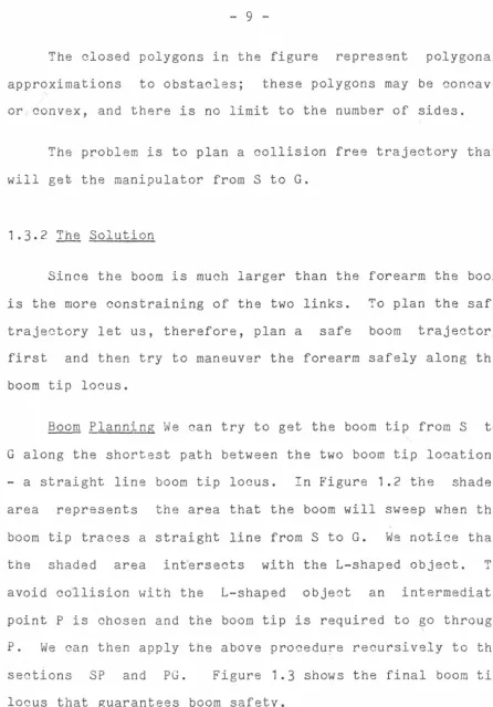
1.3.2 The Solution
Since the boom is much larger than the forearm the boom
is the more constraining of the two links. To plan the safe
trajectory let us, therefore, plan a safe boom trajectory
first and then try to maneuver the forearm safely along the
boom tip locus.
Boom Planning We can try to get the boom tip from S to
G along the shortest path between the two boom tip locations
- a straight line boom tip locus. In Figure 1.2 the shaded
area represents the area that the boom will sweep when the
boom tip traces a straight line from S to G. We notice that
the shaded area int'ersects with the L-shaped object. To
avoid collision with the L-shaped object an intermediate
point P is chosen and the boom tip is required to go through
P. We can then apply the above procedure recursively to the
sections SP and PG. Figure 1.3 shows the final boom tip
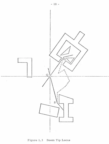
Forearm Planning Suppose boom planning ends successfully and that it finds a sequence of straight line segments such that if the boom tip travels along t0ese lines the boom will travel safely from S to G. Then if we can maneuver the forearm safely along the boom tip locus we will have found a safe trajectory for the entire manipulator. This is not easy. Furthermore, the maneuverability of the forearm near the goal configuration is very limited. This requires that the forearm be oriented "favorably" when the manipulator nears the goal.
Execution ~he above planning procedure results in a trajectory locus. Trajectory calculation routines use this trajectory locus to generate a trajectory. The executive system in charge of operating the hardware uses this trajectory to move the manipulator.
Embellishments Planning can be phases called mid-section phase
simpler trajectory.
1.3.3 Discussion
The safe trajectory planning problem deals with finding
one safe trajectory from an infinite set of safe
trajectories. This latter set is a subset of the set of all
trajectories the manipulator can execute. Computing a
member of or determining membership in this set of safe
trajectories is a computationally expensive affair. Thus
anyone hoping to find a solution to the safe trajectory
planning problem has to determine how to reduce the size of
the search space and how to keep the computation tractable.
The following is a list of questions, the answers to
which will provide a solution to the collision avoidance
problem.
1) How can collision checking be done efficiently? If
the physical dimensions of manipulator links ·are included,
collision detection becomes even more expensive. Are
simpler descriptions of the manipulator possible?
2) How should the initial trajectory hypothesis be
done?
3) On detection of a collision how should trajectory
modification be done?
irregular shapes, to be represented? Intuitively we feel
that maneuvering far away from obstacles should be easy. Is
it possible to realize this expectation in a computer
program?
5) Is the problem of safe trajectory planning better
dealt with as planning trajectories in free space rather
than as a collision detection and avoidance problem, or is a
judicious choice of both approaches possible? How then does
one represent free space?
6) What are good tiprimitives" for trajectories? The
primitives should simplify collision checking and make easy
trajectory hypothesizing and modifying.
7) Obstacles are naturally described in cartesian space
and trajectories in joint space. Since the two are
represented in different spaces, collision checks require
constant and expensive conversion between the two spaces.
Should obstacles, therefore, be described in joint space or
should trajectories be represented in cartesian space, or is
it possible to use both spaces judiciously?
8) What are good planning heuristics? Should we use
the same heuristics for maneuvering close to obstacles and
far away from obstacles?
9) If safe trajectory planning is irreparably complex
(computationally speaking) can some part of the planning be
necessary data for execution-time planning? What should
these sensors be?
This dissertation provides satisfactory answers to the
questions raised here. These answers provide solutions to
the colLision detection and avoidance problem and make it
numerically tractable. The solution is described for
manipulators with a sliding joint (see Figures 3.1-3.5).
1.4 HISTORICAL PERSPECTIVE
Collision avoidance problems became manifest when
computer controlled manipulators came into existence during
the mid~sixties. Pieper(1968) was one of the first to
investigate the problem. Paul(1972) did some ex~ellent work
on trajectory calculation and servoing. Lewis(19'74) applied
Paul's work to the JPL manipulator and also tackled the safe
trajectory planning problem. Widdoes(1974) made by far the
most serious attempt at the problem of collision avoidance.
None of these earlier attempts could handle the complexities
similar to the ones illustrated in the example of Figure
1.1. A comparison of my solution to the safe trajectory
planning problem, with those of Pieper, Lewis and Widdoes is
1.5 OVERVIEW OF THE REPORT
This dissertation presents the solution to the safe
trajectory planning problem at a number of different levels.
The reader may choose to stop at any level and he should
have a , good understanding of the solution. If he is
interested in knowing more he can go to the next level of
detail. A necessary consequence of such an approach to
describing anything is repetition. Definitions,
descriptions of motivation, representations, algorithms etc.
get repeated and are presented in greater detail and often
in a slightly different context. The reader who plans to
read the entire thesis should be prepared for this.
The problem l am interested in is the safe trajectory
planning for the 3D manipulator. To simplify thB problem I
first solved the problem for a two-dimensional manipulator.
Though a simple generalization to three dimensions is not
possible, the solution to the two-dimensional problem was
very useful in coming
three-dimensional problem.
up with a solution to the
Chapter 2 provides a theoretical framework for the
solution to the collision detection and avoidance problem.
For a casual reader interested in knowing the main features
of the solution, chapters 2 and 11 should suffice. Chapter
problem.
The presentations in chapters 3-9 follow a uniform
pattern. The first few sections deal with the motivation
and matters of general interest to both the two- and
three-dimensional problems. This is followed by the
solution to the 2D problem, and a discussion of the natural
generalization of the 2D solution and the problems, if any,
with such a generalization. The solution to the 3D problem
concludes the chapter. Chapters 3-6 explore the models of
different entities in the universe of discourse. They
include the manipulator, the obstacles in the environment,
the free space available for maneuvering, and trajectories.
Chapter 7 discusses goal feasibility analysis, Chapter 8
trajectory planning in regions relatively far removed from
obstacles and Chapter 9 discusses trajectory planning closer
to obstacles.
Chapter 10 presents system details and a critical
review of the 2D and 3D implementations. Chapter 11
concludes the report with a presentation of the key ideas of
the solution and discusses some directions for future work.
Appendix 1 gives a brief descriptiqn of the JPL robot.
Appendix 2 describes an ordering relation. Appendix 3
\
:
I
I jI
0
v
.
·-
·
-
--
-
·
-
;r
. ---
----
-
--
----
-
-
----
-
·
-
--
-
·-
-
·
·
--
--
-
-
--
-
-
-
-
-
--
-
-
-
-
----
-
-
--
-i
I
i
I
I
I
I
_
__ _j
CHAPTER 2
A THEORETICAL FRAMEWORK
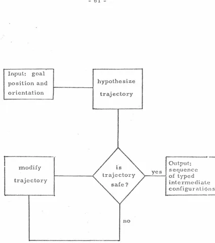
The trajectory planning task may be pictured as shown
in the flowchart of Figure 2.1. The manipulator system on
initialization is given a description of the environment.
The environment will change due to the manipulator picking
up, transporting and putting down objects elsewhere. The
environment may also be reinitialized to something
completely new. It is assumed that such reinitializations
are infrequent compared to the total number of trajectories
planned. This assumption is referred to as the infrequent
environment initialization hyoothesis.
The input consists of the position and orientation of
the manipulator for the goal configuration. The output is a
list of typed intermediate configurations, the type
indicating the nature of the subsequent section of the
trajectory. The trajectory calculation program· uses these type specifications when generating trajectories to run the
hardware.. The first step in the planning process is to hypothesize a trajectory. Following this is an iterative
step which checks for collisions. If there is potential
danger, the proposed trajectory is modified and the
iteration continued. If the trajectory is safe the planning
-hypothesize and modify trajectories, and check collisions
in greater detail.
The routines that hypothesize and modify trajectories
will find it very convenient to have a good characterization
of 1) Large empty spaces, because a trajectory designed to
pass through large empty spaces is very likely to be safe.
2) Terminal obstacle configurations, since special
heuristics can be associated with different obstacle
configurations, thereby increasing the chances of proposing
a collision free trajectory at the first try. What are good
representations for empty spaces and obstacles? What are
good heuristics for hypothesizing trajectories? How and
where should trajectory modification be effected so that the
same problem does not recur, and that new problems do not
arise? This dissertation provides answers to these
questions.
Collision detection has its own problems, making it
computationally expen~ive. Since it is a computation which
is repea~ed many times it is essential to make this step
efficient. Trajectories are most conveniently described in
joint variable space while obstacles are described naturally
in cartesian space. When the manipulator moves, its links
trace a volume in cartesian space called the traieatory
intersections of the trajectory envelope (represented in
joint variable space) and obstacles (represented in
cartesian space). Since the two are represented in
different spaces, intersection checks require constant
conversion between the two spaces. This makes the checks
expensive and is referred to as the conversion overhead
problem. Should obstacles, therefore, be described in joint
variable space or should trajectories be represented in
cartesian space or is it possible to use both spaces
judiciously? This thesis ShOHS how it is possible to use
the best of both the joint variable and cartesian space
representations. .Again, safe trajectory planning can be
viewed as a) maneuvering in free space, and b) avoiding
obstacles. This thesis shows these complementary views can
be used to advantage in solving the planning problem.
Now, the complexity of planning is a function of how
the manipulator is modelled. This thesis shows that the
manipulator can b2 modelled in a number of problem spaces of
increasing abstraction. Starting with a simple and direct
model of ~wo connected cylinders, we go to show how the
manipulator can be modelled as two connected line segments,
a single line segment, and incredibly as a point! If we
model the manipulator as two connected cylinders we will be
operating at the most complex level; with a point model of
This thesis describes the different problem spaces, their
properties, how they are generated and the relationship
between them.
The solution will be presented in two parts
representation and planning. Section 2.1 outlines the
criteria for a satisfactory solution. The last section of
this chapter is a survey of the past work as seen in the
framework of my solution.
2.1 SOLUTION CRITERIA
We are looking for a system that solves the trajectory
planning problem in a variety of obstacle configurations.
We want a system that plans safe trajectories in a time
comparable to the execution time of the trajectories, which
for the JPL robot's arm is between 5 and 10 seconds. The
system need not produce a truly optimal plan. In fact an
optimal plan is often not worth the extra computation
required to produce it. At the same time the system should
not produce blatantly stupid plans. We do not want the
manipulator to do any unnecessary acrobatics. The system
should perform well in simple and commonly occurring
situations and it may take more time on difficult problems.
It should be able to recognize when things go out of hand
2.2 hEPRESEN~ATION
The representation aims at simplifying the tasks of
hypothesizing and modifying trajectories, and 0hecking the
safety of proposed trajectories. The entities in the
universe ' of discourse that need to be represented are the
manipulator, the obstacles in the environment, the
maneuverable free space and trajectory envelopes.
The infrequent initialization hypothesis, in effect,
says that a large number of trajectories are planned for any
given environment. In view of this it is worthwhile looking
for alternative problem spaces where the computational
complexity of trajectory planning might be less.
Multiple
engineering
problem
and
spaces
science.
are extensively used
The time-domain
in
and
frequency-domain analysis of dynamic systems is a classic
example. Whenever multiple representations are used
equivalence of the representations is of great importance.
Intuitively, equivalence
existence of solutions in
of representations guarantees the
the alternative space when a
solution exists in the first and vice versa. The second
important aspect about multiple representations is concerned
The r~presentation hierarchy of Table 2.1 shows three
problem spaces. The table also describes the representation
of every entity in the world in each of the three problem
spaces. The relationship between the three problem spa~es
is described first and the individual spaces are described
next. The description of a problem space includes the
representations for the four components of the world, their
inter-relationships and how they are generated. Their use
in trajectory planning is described in section 2.3.
The first space is called the real problem space and is
closest to the real world. A solution to the trajectory
planning problem in this space is a solution to the
trajectory planning problem in the real world. The converse
is true if one ignores the fact that obstacle ~hapes are
approximated by bounding polyhedra. When a solution to the
trajectory planning problem in one space implies a solution
in the other and vice versa, the two spaces are said to be
equivalent(w).
Solving the trajectory planning problem in the real
problem space is easier than doing so for the real world.
The task, however, is still quite difficult. We therefore
identify a new space called the primary problem space, that
is equivalent to the real , problem space and wherein the
complexity of the task is greatly reduced. The reasons for
the simplicity of trajectory in the primary problem space
will be presented later. The process of generation of the
primary problem space ensures that the trajectory in the
primary problem space is identical to a trajectory in the
real world i.e. there is an identity transformation
relating the solution in the two spaces.
The primary problem space simplifies the trajectory
planning problem considerably as compared to the real
problem space. However, forearm planning is still quite
expensive and so a third space called the secondary QLOblem
space, is introduced to simplify forearm planning. The
secondary problem space admits a simple description of the
manipulator; the manipulator consists of just the boom. As
a consequence of this simplicity the primary and secondary
problem spaces are not equivalent. For, it may ha·ppen that
there is a solution to the trajectory planning problem in the primary problem space but not in the secondary space.
discussed in detail in section 2.2.3. Trajectory planning
in the secondary problem space is so simple that it more
than justifies planning in a problem space that is not
equivalent to the real world. Again, as in the primary
problem space, the process of generation of the secondary
problem space ensures that there is an identity
transformation relating trajectories in secondary space to
trajectories in the real world. The primary problem space
is an extension(*) of the secondary problem space.
The relationship between the three spaces is summarized below:
Real Problem Space
Primary Problem Space
Secondary Problem Space
where A
=>
B means a solution in space A implies a solutionin space ·B and A
<=>
B means A=>
B and B=>
A.*
The concept of extension used here is in the sense2.2.1 Real Problem Soace
Any object the manipulator is likely to collide with is
termed an obstacle. On the JPL robot (see Figure A1.1)
obstacles would include the platform, the interface
electron{cs rack, the TV and laser rack, the wheels and
their motors etc. If the robot is operating in an outdoor
environment a boulder within the manipulator's reach would
be considered an obstacle. Some of the obstacles have well
defined geometric shapes such as parallelepipeds, cylinders,
toroids etc. Others, especially natural obstacles are very
irregular in shape. Since collision detection involves
determining intersection of shapes, the more complex the
shape, the more the computational effort. Also, the less
succinct the description, the more will the storage
requirements be. To reduce the storage requirements and the
computational time for intersection checking, the obstacles
are replaced by their enclosing polyhedra. These polyhedra
may be concave or convex. There is also no limit on the
number of faces and thus the approximation by polyhedra can
.
be accurate to any arbitrary degree. The sst of polyhedra,
each approximating a real obstacle, is called the map.
The maneuverable soace is the complement of the volume
occupied by elements of the map, with respect to the
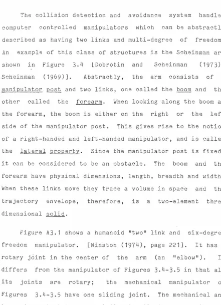
The collision detection and avoidance system handles
computer controlled manipulators which can be abstractly
described as having two links and multi-degree of freedom.
An example of this class of structures is the Scheinman arm
shown in Figure 3.4 LDobrotin and Scheinman (1973),
Scheinman (1969)]. Abstractly, the arm consists of a
manipulator post and two links, one called the boom and the
other called the forearm. When looking along the boom at
the forearm, the boom is either on the right or the left
side of the manipulator post. This gives rise to the notion
of a right-handed and left-handed manipulator, and is called
the lateral property. Since the manipulator post is fixed,
it can be considered to be an obstacle. The boom and the
forearm have physical dimensions, length, breadth and width.
When these links move they trace a volume in spac~ and the
trajectory envelope, therefore, is a two-element three
dimensional solid.
Figure A3.1 shows a humanoid "two" link and six-degree
freedom manipulator. [Winston (1974), page 221]. It has a
rotary joint in the center of the arm (an "elbow"). It
differs from the manipulator of Figures 3.4-3.5 in that all
its joints are rotary; the mechanical manipulator of
Figures 3.4-3.5 have one sliding joint. The mechanical and
2.?.2 Primary Problem Space
The primary problem space admits simplified manipulator
descriptions which simplify trajectory planning while still
maintaining equivalence with the real problem space.
Instead ' of considering the manipulator as consisting of two
solid links, the manipulator is viewed as consisting of a
single line segment and having no lateral property. In
order to preserve the equivalence with the real problem
space, appropriate transformations are made on the obstacle
and maneuverable space descriptions. It is very essential
that these transformations have the following minimality
property: the transformations need to be computed only once
or if this is not possible then the number of times the
transformation is computed should be far less than the
number of trajectory computations. Otherwise the advantage
gained by using the simplified representation would be lost
in the generation of the representation.
Consider the minimum bounding cylinders for the boom
and the forearm. The finite axis of the cylinder bounding
the forearm is the single-line segment model of the
manipulator. I will now describe how such a simple view of
the manipulator lS possible while still preserving
First consider a two-line segment model of the
manipulator. The finite axes of the cylinders bounding the
boom and forearm are used for this model. In order to
preserve equivalence we enlarge the obstacles. Let k be the
radius of the cylinders. , Each polyhedron in the map is
subject to the enlarge transformation. The transformation
generates a new polyhedron such that every point on the
surface of the new polyhedron is at least a distance k away
from the nearest point on the surface of the old polyhedron.
The enlarged polyhedron is called a primary obstacle. The
set of primary obstacles is called the primary map. With
line-segment models of the manipulator links, the trajectory
envelope is now two connected surfaces, one called the boom
surface and the other the forearm surface. The maneuverable
space is called primary free space and is the complement of
the volume occupied by primary obstacles with respect to the
manipulator's workspace. The original collision detection
and avoidance problem is equivalent to the simplified
collision detection and avoidance problem for the line links
and the . enlarged obstacles of the primary problem space.
The enlargement transformation needs to be done just once.
Next, in order to ignore the lateral property of the
manipulator and still maintain equivalence between the real
and primary problem spaces, appropriate one-time-only
a right primary map. The polyhedra descriptions in these
maps reflect the manipulator characteristics. This finer
classification of maps was left out of Table 2.1 so as to
keep the table simple.
Finally, the single element description of the
manipulator is made possible by a transformation called
survey which permits the boom to be viewed as a single point
instead of a finite line segment. The trajectory envelope
will then be the forearm surface generated by the motion of
the forearm line segment. Survey when applied to free space
results in a chart. The nomenclature sterns from the use of
charts for navigation. A chart generated to represent
primary free space is called a primary chart. To see what
survey does we start with primary free space. Consider the
set of all points in the primary free space such that the
entire boom is safe from collision if the boom tip were
positioned there. This subset of free space is called
navspace (for navigational space). ~he survey
transformation approximates navspace by boxes in r-theta-phi
space cilled regions and the set of regions is called a
chart. Corresponding to the left and right primary maps we
have the left primary chart and the right QTimary chart.
Again, to keep matters simple, the finer classification of
Regions are structured entities (see Figure 2.2). They
are made up of sectoroids and sectoroids are composed of
Bases. The pasc (Q£rallelepiped in ~herical coordinates)
is the smallest unit. The choice of the parallelopiped in
spherical coordinates as the unit of shape is based on how
the planning routines will use them. Pascs, sectoroids and
regions are bounded by constant phi and constant theta
surfaces. All pascs in a sectoroid have
limits. All sectoroids in a region have the
the same phi
same theta
limits. Pascs have associated with them a maximum and
minimum r value, called rmax and rmin respectively,
indicating the safe limits of the boom extension. The
difference between the maximum and minimum r value is called
the safe limit interval. Similar to pascs, sectoroids and
regions have associated with them maximum and ·minimum r
values indicating the best possible safe limits of the boom
extension. A region, sectoroid or pasc is considered
impassable if the safe limit interval is l~ss than some
prespecified value.
Regions essentially are an approximation to the points
in navspace. This approximation is dynamic and can be
changed by higher level programs. The approximating
procedure is called refinement, and the refinement level is
called resolution. The system can refine areas where the
while elsewhere the resolution may be quite crude. This
flexibility is very useful because refining every part of
free space to the finest level possible is expensive and
often quite unnecessary. This flexibility permits the
system t~ decide where refinement is essential and what the
resolution should be. If the resolution of a particular
part of the environment is not adequate, the system can
refine that portion of the maneuverable space. This is
termed the selective refinement capability. As a result of
this capability, the survey transformation is not a one-time
operation. This is the price that has to be paid for the
flexibility. Since there is a limit to the precision of
placement of the hardware the process of refinement will not
continue indefinitely. The data structures generated during
the refinement process are saved for reuse. Selective
refinement makes incremental modifications to the chart very
inexpensive. Incremental modifications are necessitated by
minor changes in the environment that might result from the
transporting of objects from one place to another.
The concept of navspace permits considering the boom as
a single point. Navspace and its approximation by charts is
thus crucial to safe trajectory planning. The reason for
imposing a structure on charts is to have some selectivity
in terms of what parts of navspace should be refined and to
of a region and its components is irrelevant to the concept
of navspace and collision checking. The choice of boxes in
r-theta-phi space as the unit is dictated by the choice of a
particular planning strategy described in section 2.3.3.
The concepts , of navspace and charts, however, are
independent of planning strategies.
2.2.3 Secondary Problem Space
In the primary problem space the manipulator was viewed
as a single line segment with no lateral property. The
secondary problem space admits a still simpler description
of the manipulator a single point. Unfortunately, as
mentioned earlier, the secondary problem space
representation is not equivalent to the primary problem
space. However the primary problem space can be made an
extension of the secondary space and to do so appropriate
transformations are made on primary obstacles. As before we
require that these transformations satisfy the minimality
property (see section 2.2.2).
First consider the two line segment model of the
manipulator. The finite axes of the cylinders bounding the
boom and forearm are used for this modet. Suppose we ignore
the forearm. The trajectory envelope will be the boom
The polyhedra in the primary map are enlarged by the length
of the forearm. This enlargement results in secondary
obstacles and a secondary map. The maneuverable .space is
called secondary free space and is the complement of the
volume occupied by the secondary obstacles with respect to
the manipulator's work space.
The single point description of the manipulator is made
possible by applying the survey transformation to secondary
free space resulting in a secondary chart. Secondary charts
are composed of secondary regions. Whenever the boom tip is
in a secondary region the following are true 1) by
definition of the region the entire boom is free of
collisions, and 2) since secondary regions are generated
using secondary obst~cles, the forearm is .free from
collision irrespective of its orientation. The trajectory
envelope at this level then is the line generated by the
motion of the boom tip. A complex two-element trajectory
solid has thus been reduced to a line. The refinement
process for secondary charts is similar to primary charts
and so are all the attributes and transformations discussed
in the context of primary charts. In secondary problem
space too, there are left and ri~~ secondary~ and left
and right secondary charts.
the finer classification
2. 1 .
Again, to keep matters simple,
If the manipulator needs to maneuver close to
obstacles, secondary problem space is of no use. The
"gross" representation of the forearm results in the system
complaining that trajectories close to obstacles are not
feasible. Of course this does not mean that a trajectory
'
necessarily does not exist. The finer model of the forearm
as a line segment (as in primary problem space) should
result in better performance. This is what I meant when I
said that if a solution to the trajectory exists in
secondary problem space then there is a solution in primary
problem space, while if there is no solution in secondary
problem space it does not mean there is no solution in
primary problem space. Equivalently, the above remark is
same as saying that every safe trajectory in primary problem
space need not be a safe trajectory in secondary problem
space.
Looked at slightly differently, the ideas of secondary
problem space representations (the secondary charts in
particular), are a formal characterization of the intuitive
ideas of ease of maneuvering in large chunks of empty space
far away from obstacles. The reduction of the trajectory
solid to a line makes the expectation come true. Since,
close to obstacles, secondary problem space representations
are not fine enough, primary problem space representations
representations the trajectory envelope is a surface and
this is in accordance with our intuitive feeling that
maneuvering close to obstacles is not as easy as maneuvering
far away from them. A judicious use of se8ondary and
primary , problem space representations will significantly reduce the search space for good candidate trajectories, and
considerably simplify the collision detection and avoidance
task.
Left and right primary maps, and left and right
secondary maps were described as four different entities,
and so were the charts. For efficiency considerations, in
the implementation, left and right primary obstacles are
grouped together, and so are left and right secondary
obstacles. With charts, the primary and second~ry regions
are grouped together while the left and right regions remain
distinct.
2.2.4 Trajectory Envelooes
The,discussion of the three problem spaces showed how
simpler and simpler manipulator descriptions reduced the
complexity of the trajectory envelope from the two-element
solid to a single surface, the trajectory surface, or even a
single line, the trajectory trace. Collision detection
trajectory envelope and the obstacle faces. The complexity
of this task depends on the nature of the trajectory
envelope. It is therefore imperative that we look for
additional constraints to further reduce the complexity of
collision checking. Since obstacle faces are planes in
cartesian space, if the trajectory surface (trace) were a
plane (line) in cartesian space, collision checking would be
simple.
Since the manipulator hardware permits each of the
joints to be operated independently it should be possible to
get the boom tip to trace cartesian space straight lines.
However, planning cartesian space straight line loci for the
boom tip is beset with computational problems. We choose
therefore to settle for a boom space straight line locus for
the boom tip. Boom space is the subspace of joint variable
space generated by the three boom joint variables. This
straight line in boom space can then be approximated by a
sequence of straight lines in cartesian space. Safety of
the boom tip locus guarantees the safety of the entire
manipulator only when the locus passes through a secondary
chart. Elsewhere the trajectory envelope is still a surface
and, to make collision checking tractable, constraints on
forearm motion have to be introduced. We choose the
following trajectory primitives for the forearm. When the
in cartesian space parallel to the approximated boom tip
locus, and when the boom tip is stationary the forearm shall
move in a single plane. These constraints on the boom and
forearm result in the decomposition of the trajectory
surface into a sequence of parallelograms and sectors of a
circle, enormously simplifying the collision detection task.
2.2.5 Concluding remarks
The primary and secondary problem space representations
along with the restrictions on the nature of the trajectory
make the trajectory planning problem numerically tractable.
Precisely how these representations are used in planning is
described in the next section.
2.3 PLANN:NG
The first step in the planning process is to
hypothesize a trajectory. Following this is. an iterative
step which checks for collisions. If there is potential
danger, the proposed trajectory is modified and the
iteration continued. If the trajectory is safe the planning
is over (see Figure 2.1). The central aim is to reduce the
planning time. It is therefore essential that very few
errors be made during trajectory hypothesizing and
fix-ups that the system can ill afford.
Hierarchy, separability and reversibility are the key
concepts in planning. The principle of reversibility states
that if a trajectory from S to G is collision free then the
same trajectory backwards from G to S is also collision
free. Hence for collision detection and avoidance it does
not matter whether a trajectory from S to G or G to S is
planned. Separability means the decomposition of the goal
into disjoint, reasonably independent parts. Hierarchy is
used in the usual sense. For each part of the goal the most
important aspects are tackled first
next. This is applied to every stage of
and the lesser ones
the process. If
some decisions made at a higher level do not pan out, local
corrections are made. If the local fix-ups do not solve the
problem the system returns to the next higher level for
replanning. Some indication as to what went wrong is
preserved and is used during subsequent attempts at
planning. At each stage it is ensured that the system will
terminate its activities in a finite amount of time. If the
system is not successful in solving the problem it gives up
and asks for human help.
The goal is specified
orientation of the forearm.
as a 3-space position and
The position problem for the
place the manipulator in the goal configuration are
determined and the ones corresponding to the starting
manipulator configuration (same lateral configuration) are
chosen.
2.3.1 Two Approaches
Conceptually, since the trajectory envelope has the
simplest description in the secondary problem space,
planning should start in that space. Having planned as much
of the trajectory as possible in the secondary problem
space, the system should attempt to plan the rest of the
trajectory in the primary problem space. In both spaces the
system should use the principles of hierarchy and
separability. The main drawback of this appro~ch is that
the problem of interfacing between the two spaces has no
easy solutions.
Another approach to planning is the following Plan
the boom trajectory in primary problem space. For parts of
the boom tip locus that lie within the secondary chart (of
secondary problem space) no forearm planning needs to be
done. For the remaining forearm planning is
carried out. Instead of starting with secondary problem
space and then going over to primary problem space, the
partial solution in primary problem space is "refined" using
the secondary problem space. This alternative way of
looking at the trajectory planning problem solves the
interface problems that plagued the first scheme. The
details of the second approach will now be presented.
2.3.2 Overview of Planning
The trajectory planning problem is separated into three
phases. The first is a goal feasibility analysis phase, the
second is the mid-section planning phase and the last is the
terminal planning phase. At the feasibility analysis stage,
the goal feasibility is checked and any necessary
refinements of the charts are carried out. The terminal
phase activities use the reversibility principle and plan
trajectories near the initial and final configurations. The
mid-section phase deals with midway trajectory planning.
For the terminal phase, forearm and boom planning iterate
until a satisfactory boom tip location for starting the
mid-section trajectory is found. For the mid-section,
planning proceeds hierarchially. Boom trajectory is first
planned using the primary charts alone. For portions of the
boom tip locus that do not lie in the secondary chart,
forearm planning is done. The separability principle is
used in boom planning; the trajectory for the theta-phi
If a safe forearm trajectory cannot be found, the
nature of the problem is identified and is used to revise
the boom trajectory and another attempt at forearm planning
is made. If the system is unable to come up with a safe
trajectory even after a prespecified number of attempts, it
resorts to a configuration switch.
used to plan a trajectory to get
goal, this time however, in
The same techniques are
the manipulator to the
a different lateral
configuration.
Initialization
If this also fails,
of the environment
the system gives up.
and each of the three
phases in planning is discussed in the next few paragraphs.
Note that planning incorporates simple strategies. It
may so happen that the system fails to find a solution when
there exists one in the real world. It is unlikely that
such situations will be encountered except in some
pathological obstacle configurations.
2.3.3 Initialization
The system is initialized with a description of the
environment. The system uses the input polyhedra and
generates primary and secondary obstacles for the left and right, secondary and primary maps. All the charts are generated for a default resolution. The regions of the
initialization needs to be done once for
environment.
2.3.4 Goal Feasibility and Impossible Situations
every new
Goal feasibility is done before planning begins. It
includes boom placement and forearm placement safety checks.
It determines whether the boom tip lies within a pasc of a
primary region. If not the appropriate region is ·repeatedly
refined until either the goal boom tip position is within a
pasc or the resolution limit is reached and the system
returns complaining that the goal is not feasible. The
forearm feasibility study involves checking whether in the
final configuration the forearm is safe from collision. If
the forearm is not safe the goal is deemed not feasible.
During mid-section phase boom planning, the system
keeps a watch for situations which would get the boom stuck.
If the boom cannot be maneuvered out of an area, the system
complains. Again, during forearm planning along a proposed
boom tip locus, the system looks out for situations which
would get the forearm stuck. The system requests a boom
trajectory refinement if this happens. Such situations are