Working Title: Understanding landscape influences on aquatic fauna across the central and southern Appalachians
Running Head: Landscape influences on aquatic fauna in south and central Appalachians
Keywords: Aquatics; Modeling; Boosted Regression Trees; Appalachians
Authors:
R. Daniel Hanks
Department of Forestry and Environmental Conservation Clemson University
Clemson, South Carolina 29631 rhanks@clemson.edu
Paul B. Leonard
Arctic Landsape Conservation Cooperative Science Coordinator Office of Science Applications
U.S. Fish and Wildlife Service Fairbanks, Alaska 99701 paul_lenoard@fws.gov
Robert F. Baldwin (Clemson University) R. Daniel Hanks
Department of Forestry and Environmental Conservation Clemson University
Clemson, South Carolina 29631 baldwi6@clemson.edu
Abstract: Understanding influences of multiple stressors across the landscape on aquatic biota is important for conservation, as it allows for an understanding of spatial patterns and informs stakeholders of significant conservation value. Data exists for land use/landcover (LULC) and other physicochemical components of the landscape throughout the Appalachian region yet biological data is sparse. This dearth of biological data relative to LULC and physicochemical data creates difficulties in making informed management and conservation decisions across large landscapes. At the HUC12 watershed scale we sought to create a single score for both abiotic and biotic values throughout the central and southern Appalachian region. We used boosted regression trees (BRT) to model biological responses (fish and aquatic macroinvertebrate variables) to abiotic variables. Variance explained by BRT models ranged from 62-94%. We categorized both predictor and response variables into themes and targets respectively to better understand large scale patterns on the landscape that influence biological condition of streams. We combined predicted values for a suite of response variables from BRT models to create a single watershed score for aquatic macroinvertebrates and fish. Regional models were
<A>Introduction
Assessing biological condition of rivers and streams has been performed at various spatial scales and grains. As data availability and computing power both increase, the ability to perform spatial analysis across large geographic extents and at small grain size is increasing. Examples of large scale spatial analyses across the United States include; Esselman et al. (2013), who used fish as indicators, the US Environmental Protection Agency’s Wadeabe Stream Assessment (2006) which included benthic macroinvertebrates and fish as indicators, and Hill et al. (2017) who modeled biological stream condition across the conterminous U.S. based on anthropogenic and natural watershed features. Multimetric indices (MMIs) are commonly used in studies that attempt to understand anthropogenic influences on the condition of biological aquatic
communities over vast geographies (Harris and Silveira, 1999; Hering et al., 2004; Pont et al., 2006; Pont et al., 2009). Multimetric indices use taxonomic and functional metrics that are known to be sensitive to gradients of anthropogenic disturbance as a means of assessing the health of aquatic systems.
Landscape-scale analyses are important as they cross jurisdictional boundaries and make efforts to more fully understand anthropogenic stressors on biological and ecological needs of species, populations, and communities across broad spatial extents which are often not
represented in more regional analyses. We define landscape scale as the spatio-temporal extent that allows for multigenerational population processes to occur. Such large scale analyses require extensive data that is representative across taxonomic groups through both space and time and physicochemical conditions must be represented that range from natural to extensive
(predictor variables). It is often difficult to ensure such consistency due to biological and environmental datasets being expensive to obtain, varying goals and objectives from entities collecting data, and varying monetary support for such collections. This often results in either poor spatial coverage and spatially clumped data or both. To overcome these difficulties data sets are often combined from various collection programs. However, this can result in data existing at varying taxonomic levels, problems with standardization of sampling protocols, and biases associated with site selection. For example, site densities may be more dense in some areas than others resulting in biases towards trends that are prevalent in heavily sampled areas. Angermeier and Smogor (1995) found that sampling effort influenced accuracy and precision of estimates of biological community attributes.
Anthropogenic induced stressors often correlate strongly with biological conditions of aquatic systems and thus landscape-scale analyses typically aim to use land cover and land use practices over large geographies as surrogates for local environmental conditions to provide insight into biological conditions of streams and rivers. Use of such analyses allow broad geographic scale understanding of the existing gradients of poor-to-good biological condition and the environmental factors that affect them. This aids in identifying landscape-scale stressors that further the ability of conservation practitioners, managers, and regulators to take actions which positively impact aquatic fauna through a greater understanding of large-scale stressors. However, over such great spatial extents the biological responses to anthropogenic stressors can be regionally variable and the result of local biogeographical interactions with natural and anthropogenic stressors over expansive time periods (Esselman et al. 2013).
methods (Bramblett et al. 2005; Esselman et al. 2013; McCormick et al. 2001; Stoddard et al. 2008). Biological condition indices should sufficiently cover the range of environmental
gradients, exhibit low temporal variability to repeated visits to the same site(s), and demonstrate high responsiveness to environmental degradation. Indicators that do not meet these
requirements should be excluded from analyses (Stoddard et al. 2008; Whittier et al., 2007). Use of the screening methods provided by Whittier et al. (2007) and Stoddard et al. (2008) allow a large set of contending predictor variables to be winnowed down to a smaller, manageable group of indicators used to describe the biological condition gradient in a consistent manner across regions.
Multimetric indices (MMI) combine a variety of biological indicators and indices. . Using boosted regression trees (BRT; Elith et al. 2008), we developed watershed-based MMIs that combined fish and aquatic macroinvertebrates across the Appalachian Landscape Conservation Cooperative (App LCC) region (see methods for full description) using methods developed by Stoddard et al. (2008) and Whittier et al. (2007). Additionally, we aimed to identify large scale themes that structure biological communities and thus biological condition across this large geography. The App LCC encompasses biologically important aquatic ecosystems (e.g., Tennessee and Mobile Rivers) and is predicted to undergo continued land conversion, resulting particularly in increased urbanization (Terando et al. 2014). Using broad scale land use
information to develop models to predict biological condition of streams and watersheds provides the opportunity to predictively map spatially explicit biological condition across large geographic regions (Hill et al., 2017; Carlisle et al. 2009). An understanding of the
Thus, modelling and mapping the current biological condition and developing an understanding of threats to conservation across the region is an important step towards identifying conservation opportunities and needs so that conservation practitioners can act accordingly.
<B>Methods
Our study focused on the rivers, streams, and landscape encompassed by the Appalachian Landscape Conservation Cooperative (App LCC). The App LCC is comprised of 592,129 km2, 266,307 HUC 12 watersheds, and intersects 15 states ranging from central New York to the north, and central Georgia, Alabama, and Mississippi to the south. The eastern most extent reaches western New Jersey in the north and the western most portions of North and South Carolina, while reaching as far west as southern Illinois. The topography and habitat of the region are complex over such a large land area which is comprised of six Level II ecoregions (U.S. EPA), 11 Freshwater Ecoregions, and seven major river basins and has been greatly
influenced by the lack of glaciation and ancient geology which gave rise to high levels of aquatic biodiversity. The App LCC region encompasses some of the most biologically diverse
freshwater fish resources in the United States. This is particularly true in the southwestern portion of the region. As the 19th and 20th centuries have progressed, aquatic diversity has been impacted by anthropogenic activities ranging from agricultural practices, land conversion, and extractive industries.
Landscape data used as predictors
and conservation practitioners we identified 52 predictor variables comprising six themes that are known to influence fish and aquatic macroinvertebrate communities (Appendix Table 1A). Themes included streamflow, geomorphic condition, connectivity, water quality, non-point source pollution, and point source pollution and were established and evaluated to understand large scale thematic processes that influence aquatic biota across the App LCC. Predictor data were compiled from regional and national datasets at the National Hydrography Dataset version 2 (NHD+V2) HUC12 watershed level (Final predictors used in BRT models are shown in Table 1; Comprehensive list of predictor data with source provided in Appendix A). Riparian corridors are known to be influential for developing ecological diversity (Naiman et al., 1993) and in structuring aquatic communities; hence, we used The Nature Conservancy’s Active River Area (Smith et al., 2008) as a buffer into which land cover variables were clipped for modeling. The active river area framework provides an ecologically sound modelling mechanism to capture important variables that structure aquatic ecosystems (Smith et al., 2008). We centered and scaled all predictor variables to overcome instances where predictor variables had wide ranges resulting single predictors dominating models.
Fish and macroinvertebrate data
community dataset was comprised of 2,991 sample sites across the region and was somewhat sparse (2,991 locations within 266,309 HUC12 watersheds = 1.1%) but exhibited good spatial distribution (Figure 2). Our aquatic macroinvertebrate dataset was comprised of only 194 sampling locations and had poor spatial coverage (194 locations of 266,309 HUC12 watersheds = 0.07%) and distribution across the region (Figure 2).
For fish we calculated taxonomic richness and diversity and several functional group metrics using the fish traits database provided by Frimpong and Angermeir (2009) and the tolerance database of Stoddard et al. (2005). In total we calculated 45 metrics for further
analysis of fish responses to our predictor dataset. Our final analysis used 9 of these metrics and these were further aggregated into three groupings (i.e., targets) (Table 2). For aquatic
macroinvertebrates the metrics modeled as response variables were % EPT (i.e., percent Ephemeroptera/Plecoptera/Tricoptera), % of total abundance comprised by the five most dominant taxa, % of total abundance that were tolerant taxa, and % of the total abundance that were intolerant taxa (Table 2).
Boosted regression tree models and multimetric indices
Tree complexity and learning rate were systematically altered in order to identify the optimal model structure. We reduced model complexity by removing redundant variables (r > 0.80) and variables with minimum variation among sites. Global models were developed with the
remaining variables and then further simplified using scree plots of the predictor relative
influence. Simplified models were retained if their cross-validation was greater than or equal to that of the global model. BRT models were developed with methods and code provided by Elith et al. (2008). Initial analyses were performed across the entire geography without accounting for regional differences (i.e., ecoregions) but due to a clear need for the inclusion of regional
differences within the models we used Freshwater Ecoregions of the World (Abell et al. 2008) to understand these regional differences. Freshwater ecoregions attempt to place aquatic
ecosystems in a biogeographical framework based on ecological and evolutionary patterns of fish distributions (Abell et al. 2008). Due to low sample site numbers in some Freshwater
Ecoregions we aggregated the 11 ecoregions that comprised the App LCC into four. The four aggregated ecoregions and their composite Freshwater Ecoregions were Atlantic Slope
(Appalachian Piedmont, Chesapeak Bay, Northeast US and Southeast Canada Atlantic Drainages), Cumberland (Cumberland River Basin), Ohio (Teays-Ohio and Laurential Great Lakes River Basins), and Tennessee (Tennessee and Mobile Bay River Basins). Regional models were successfully run for fish but due to the lack of spatial coverage, we were unable to model aquatic macroinvertebrates regionally and we therefore retained models for the entire geography for aquatic macroinvertebrates.
aquatic macroinvertebrate scores. Boosted regression trees provide the relative influence of predictor variables in the modelling of responses and we averaged these relative influences within our thematic framework (see above and table 1) for each fish and aquatic
macroinvertebrate response variable.
<C>Results
The screening process reduced the total number of predictor variables to 37 from 52. When predictor variables were correlated, we attempted to retain the variable most responsive to our models; however, this was not formally tested. The themes with the greatest number of predictor variables were non-point source pollution and point source pollution (each with eight variables). While the theme with the least number of predictor variables was geomorphic condition (two variables) (Table 1).
Below, we present results from the boosted regression tree models where the models were run with all ecoregions together for both fish and aquatic macroinvertebrates. We refer to this as a “Global” model (see below). After which, we present results where separate models were run for each Freshwater Ecoregion (defined in the materials and methods section). We refer to these models as regional models and because there were not enough data points within the regional data sets for aquatic macroinvertebrates, they were developed for fish only.
Global models
Boosted regression tree models were developed for 45 % (28/62) of the response variables; however, we only retained 12 (eight and four response variables for fish and aquatic
targets (Shannon diversity, functional group, and taxa quality) and for aquatic macroinvertebrates we retained macroinvertebrate taxa quality as the only target.
The range of deviance explained by the BRT models was 48 % for percentage of invertivore taxa to 85 % for fish taxa diversity (x̄ = 73 %) for fish and 76 % for percentage of the five
dominant taxa to 89 % for percentage of tolerant taxa (x̄ = 81 %) for aquatic macroinvertebrates. For the fish BRT models, the cross-validated deviance ranged from 32 % for percentage of invertivore taxa to 69 % for fish taxa diversity (x̄ = 52 %), while for aquatic macroinvertebrates it ranged from 24 % for percentage of the five dominant taxa to 76 % for percentage of tolerant taxa (x̄ = 41 %). The lower cross validated deviances for aquatic macroinvertebrates relative to those of fish, are likely due to the lack of spatial data coverage in the aquatic macroinvertebrate data (Figure 1 b).
Based on the results of the BRT models, the predictor variables that had the greatest relative influence were freshwater ecoregion and network percent impervious surface for fish and aquatic macroinvertebrates respectively. Those with the least relative influence were CONF_CL and watershed mine density for fish and aquatic macroinvertebrates respectively. The theme with the greatest cumulative relative influence for fish was geomorphic condition (46.6 %) and for aquatic macroinvertebrates was water quality (41.7 %), while point source pollution was the least important theme for both fish (1.4 %) and aquatic macroinvertebrates (0.8 %) (Table 4). The relative thematic influence was variable between response variables; where, for example the flow theme was the most influential for % EPT (27.4 %) but for % intolerant taxa the most influential theme was water quality (87.9 %).
Regional differences were evident in the results of the relative influence of predictor variables on responses. For example, the variable with the greatest relative influence for richness in the Atlantic Slope data was July temperature (22.8 %), for the Cumberland River Basin was ground flow recharge (17.6 %), for the Ohio River Basin was average catchment elevation (21.4 %), and for the Tennessee River Basin it was dam storage capacity (8.2) (Table 6). Additionally, the relative influence varied widely within a given region for the same predictor variable but for different response variables. For example, k-factor (a measure of soil erodibility) had the 24th most influence on diversity in the Atlantic Slope but was the 4th most influential variable in the
% herbivore taxa model. The standard deviation associated with the relative influence of predictor variables for a specific region was also variable; where, for example, for invertivore diversity the standard deviation was 2.4, 2.6, 5.1, and 4.3 for the Atlantic Slope, the Cumberland River Basin, the Ohio River Basin, and the Tennessee River Basin respectively.
The mean relative influence for themes were also somewhat variable across regions; where, for example, flow was the most influential theme for each region for the BRT model for the % of species that prefer coarse sediment. However, for the % of tolerant fish species the flow theme represented the 4th most influential theme for the Atlantic Slope (x̄ = 1.7 %), 3rd most for the Cumberland River Basin (x̄ = 2.5 %), 2nd most for the Ohio River Basin (x̄ = 2.7 %), and 1st most for the Tennessee River Basin (x̄ = 3.6 %).
influential theme for the Atlantic Slope, the Ohio River Basin, and the Tennessee River Basin but the 5th most influential for the Cumberland River Basin.
Fish models
Model results suggest there are distinct areas of the App LCC region that exhibit characteristics of poor biological condition (i.e., watershed score) (Figure 3). For example, western Tennessee (i.e., the Southeastern Plains) and the norther-most portion of the region (i.e., the Atlantic Highlands). Additionally, large rivers tended to exhibit poor biological condition. This was especially true in areas with high agricultural land use (i.e., east Tennessee). Regions where the models displayed relatively good biological condition were largely in areas free from agricultural land use. However, even in areas with good biological condition, large rivers exhibited poor biological condition.
Pearson correlations between the global and regional models were variable and ranged from 0.33 (% intolerant taxa) to 0.99 (% invertivore taxa) for pairwise comparisons. The overall indices for watershed scores (i.e., biological condition) were moderately correlated (0.69). The targets were highly correlated for functional group (0.98) but were relatively poorly correlated for taxa quality (0.34) (Table 8) (Figure 5).
Aquatic macroinvertebrate model
having poor biological condition, the aquatic macroinvertebrate models were unable to identify biological condition at this scale (Figure 4). Additionally, the Pearson correlation coefficient between the aquatic macroinvertebrate watershed score and those of the global (Figure 5) and regional fish watershed scores was 0.01 for both.
<D>Discussion
Freshwater ecosystems are highly threatened worldwide. In North America the Appalachian LCC region is a particularly valuable aquatic ecosystem due in large part to its high aquatic biodiversity. It is also a region of great conservation concern due to current and projected rapid land cover change (i.e., urbanization), biodiversity loss, habitat fragmentation, and climate change (Terando et al. 2014, Leonard et al 2017). Models such as the ones present here and others (e.g., Esselman et al., 2013 and Hill et al., 2017), are valuable resources for identifying areas of greatest concern for restoration activities and those areas in greatest need of increased and/or continued protection.
Multimetric indices may be beneficial in identifying biological condition across large geographies. Our results suggest that multimetric scores (i.e., watershed scores) corroborate one another at the global and regional scales (see table 8), indicating that the predictor variables we used were responsive in a consistent manner across scales. This is an important finding as the ability to rely on a consistent set of landscape variables enables cross-regional and cross-scale comparisons; which can be particularly important when data sets are assembled from multiple sources (Esselman et al. 2013).
regions regarding what environmental factors influence community structure. These findings are not surprising as they are congruent with other large-scale biological condition assessments (Esselman et al. 2013; Hill et al. 2017). While individual predictors were relatively variable between regions, our models suggested themes (i.e., combined predictors) were more consistent yet still exhibited some discrepancies between regions. The themes that exhibited the greatest influence on fish watershed scores across the entire region were geomorphic condition and flow regime. Geomorphic condition in our analysis was a measure of soil stability and erosivity. This finding is unsurprising as aquatic taxa are known to be sensitive to sedimentation. Surprisingly, point source pollution and connectivity were least influential. This is likely due to these two factors being measured somewhat sparsely (i.e., few watersheds have NPDES sites) on the landscape. For example, NPDES density, a measure of point source pollution, is likely to exhibit strong influence on aquatic biota in the immediate area but these sites are scattered across the landscape and thus across a large region such as the App LCC region, they were less influential in our models than predictors that are found in nearly every watershed (e.g., soil erosivity).
same sites are sampled for both. For example, at 18 sites in the River Raisin watershed in Michigan, correlations between fish and aquatic macroinvertebrate indices ranged from 0.21 to 0.51 (Lammert and Allen 1999). Additionally, stressors have been found to affect fish and aquatic macroinvertebrates similarly. Free flowing stream sections of the Fox River, IL exhibited higher index scores for both fish and aquatic macroinvertebrates when compared to sections of the river above low-head dams (Santucci et al., 2005).
Esselman et al. (2011) suggested regional stratification for analyses that span large geographies, while also including multiple biological response variables, and using statistical modeling techniques that are non-linear would lead to improved multimetric indices. This is precisely the approach we took modeling biological condition across the 15 state App LCC region. However, one major difference between our study and previous studies is that previous work to developed multimetric indices across broad geographies included regional influences by using Omernick ecoregions (Whittier et al., 2007; Esselman et al. 2013, and Hill et al. 2017). Omernick ecoregions are a spatial framework which includes aquatic and terrestrial ecosystems (Omernick 1987; USEPA 1996); however, we used Freshwater Ecoregions of the World for our analysis because they were developed on a framework that focused exclusively on aquatic ecosystems with fish as the focal taxonomic group (Abell et al. 2008).
Another difference between our work on previous work is that we aggregated both predictor and response variables into themes and targets respectively. By aggregating predictor variables into themes we were able to identify categories of predictors that were influential in structuring fish and aquatic macroinvertebrate communities in aggregate (e.g., watershed score for fish), as well as for individual response variables (e.g., % EPT). Response variable
themes) structure fish and/or aquatic macroinvertebrate communities in a more functional
manner. For example, two targets (e.g., fish functional group and fish taxa quality) may respond differently to the same stressor. Understanding which higher order stressors (theme) affect our targets (fish functional group) may lend insight into more effective regional management and conservation strategies. However, thematic importance was variable between regions and care should be taken when using large scale modeling efforts such as ours to make management recommendations across large regions that span more than one ecoregion.
While we were able to develop regional models for fish indices, we were, unfortunately, unable to develop regional aquatic macroinvertebrate models due to low numbers of sample sites. As aquatic macroinvertebrates are known to be good indicators of biological condition (Gerritsen et al. 2000; Pond et al. 2008) we believe there needs to be increased systematic sampling efforts that result in an increased number of sites that are spatially dispersed across multiple freshwater ecoregions and that includes known areas of both high and low biological integrity. With an extensive sampling approach that includes both fish and aquatic
Acknowledgments
Literature Cited
Abell, R., M. L. Thieme, C. Revenga, M. Bryer, M. Kottelat, N. Bogutskaya, B. Coad, N. Mandrack, S. C. Balderas, W. Bussing, M. L. J. Stiassny, P. Skelton, G. R. Allen, P. Unmack, A. Naseka, R. Ng, N. Sindorf, J. Robertson, E. Armijo, J. V. Higgins, T. J. Heibel, E. Wikramanayake, D. Olson, H. L. Lopez, R. E. Reis, J. G. Lundberg, M. H. Sabaj Perez, and P. Petry. 2008. Freshwater ecoregions of the world: a new map of biogeographic units for freshwater biodiversity conservation. BioScience 58(5):403-414. Angermeier, P. L. and R. A. Smogor. (1995). Estimating number of species and relative
abundances in stream-fish communities: effects of sampling effort and discontinuous spatial distributions. Canadian Journal of Fisheries and Aquatic Sciences, 52(5), 936-949.
Bramblett, R. G., Johnson, T. R., Zale, A. V., and Heggem, D. G. 2005. Development and evaluation of a fish assemblage index of biotic integrity for northwestern Great Plains streams. Transactions of the American Fisheries Society, 134(3), 624-640.Carlisle, D. M., J. Falcone, M. R. Meador. 2009. Predicting the biological condition of streams: use of geospatial indicators of natural and anthropogenic characteristics of watersheds. Environmental Monitoring and Assessment 151:143-160.
https://doi.org/10.1007/s10661-008-0256-z
Essleman, P. C., D. M. Infante, L. Wang, D. Wu, A. R. Cooper, and W. W. Taylor. 2011. An index of cumulative disturbance to river fish habitats of the conterminous United States from landscape anthropogenic activities. Ecological Restoration 29:133 -151. Esselman, P. C., D. M. Infante, L. Wang, A. R. Cooper, D. Wieferich, Y-P. Tsang, D. J.
Thornbrugh, and W. W. Taylor. 2013. Regional fish community indicators of landscape disturbance to catchments of the conterminous United States. Ecological Indicators 26:163-173.
Frimpong, E. and P. L. Angermeier. 2009. Fish traits: a database of ecological and life history traits of freshwater fishes of the United States. Fisheries 34:487-495.
Ford, T. R. ed. 2015. The Southern Appalachian Region: A Survey. Lexington: University of Kentucky Press.
Gerritsen, J., Burton, J., and Barbour, M. T. 2000. A stream condition index for West Virginia wadeable streams. US EPA Region, 3.
Harris, J. H. and R. Silveira. 1999. Large‐scale assessments of river health using an Index of Biotic Integrity with low‐diversity fish communities. Freshwater Biology, 41(2), 235-252.
Hering, D., Moog, O., Sandin, L. and Verdonschot, P. F. 2004. Overview and application of the AQEM assessment system. Hydrobiologia, 516(1-3), 1-20.
Leonard, P. B., R. F. Baldwin, and R. D. Hanks. 2017. Landscape-scale conservation design across biotic realms: sequential integration of aquatic and terrestrial landscapes. Scientific Reports, 7 Article Number 14556 doi:10.1038/s41598-017-15304-w. Lammert, M. and J. D. Allan. 1999. Assessing biotic integrity of streams: effects of scale in
measureing the influence of land use/cover and habitat structure on fish and macroinvertebrates. Environmental Management 23(2):257-270.
McCormick, F. H., Hughes, R. M., Kaufmann, P. R., Peck, D. V., Stoddard, J. L., & Herlihy, A. T. 2001. Development of an index of biotic integrity for the Mid-Atlantic Highlands region. Transactions of the American Fisheries Society, 130(5), 857-877.
Naiman, R. J., H. Decamps, and M. Pollack. 1993. The role of riparian corridors in maintaining regional biodiversity. Ecological Applications 3(2):209-212.
Omernik, J. M. 1987. Ecoregions of the conterminous United States. Annals of the Association of American geographers, 77(1), 118-125.
Pond, G. J., J. E. Bailey, B. Lowman, and M. J. Whitman. 2008. "West Virginia GLIMPSS (genus-level index of most probable stream status): a benthic macroinvertebrate index of biotic integrity for West Virginia’s wadeable streams." West Virginia Department of Environmental Protection, Division of Water and Waste Management, Watershed
Branch, Charleston, WV, USA.
Pont, D., Hugueny, B., Beier, U., Goffaux, D., Melcher, A., Noble, C. Rogers Noble, N. Roset and Schmutz, S. 2006. Assessing river biotic condition at a continental scale: a European approach using functional metrics and fish assemblages. Journal of Applied
Pont, D., Hughes, R. M., Whittier, T. R. and Schmutz, S. 2009. A predictive index of biotic integrity model for aquatic-vertebrate assemblages of western US streams. Transactions of the American Fisheries Society, 138(2), 292-305.
Santucci, V. J., S. R. Gephard, and S. M. Pescitelli. 2005. Effects of multiple low-head dams on fish, macroinvertebrates, habitat, and water quality in the Fox River, Illinois. North American Journal of Fisheries Management 25(3):975-992. doi.org/10.1577/M03-216.1. Smith, M. P., R. Schiff, A. Olivero, J. G. MacBroom. 2008. The active river area: a
conservation framework to protect rivers and streams. The Nature Conservancy: Boston, MA.
Stoddard, J. L., Peck, D. V., Olsen, A. R., Larsen, D. P., Van Sickle, J., Hawkins, C. P., R.M. Hughes, T. R. Whittier, G. Lomnicky, A. T. Herlihy, and Kaufmann, P. R. 2005.
Environmental Monitoring and Assessment Program (EMAP): western streams and rivers statistical summary. Washington, DC: US Environmental Protection Agency, Office of Research and Development.
Stoddard, J. L., Herlihy, A. T., Peck, D. V., Hughes, R. M., Whittier, T. R., & Tarquinio, E. 2008. A process for creating multimetric indices for large-scale aquatic surveys. Journal of the North American Benthological Society, 27(4), 878-891.
Terando, A. J., J. Costanza, C. Belyea, R. R. Dunn, A. McKerrow, and J. A. Collazo. 2014. The southern megalopolis: using the past to predict the future of urban sprawl in the
southeast U.S. PLOS One 9(7) e102261. https://doi.org/10.1371/journal.pone.0102261
Figure captions
Figure 1. Overview map of the Appalachian Landscape Conservation Cooperative.
Figure 2. Side-by-side comparison of response data for fish and aquatic macroinvertebrates showing spatial distribution of sample locations for both.
Figure 3. Comparison of the watershed score for the global and regional models. The watershed scores were centered and scaled. The regional watershed scores were centered and scaled within each respective region within the Appalachian LCC region. The global watershed scores were centered and scaled across the entire Appalachian LCC region.
Table captions
Table 1. List of final predictors used in boosted regression tree models and how each was grouped thematically.
Table 2. List of final responses modeled with boosted regression trees and how each was condensed (i.e., averaged and grouped) into an average score to represent larger taxonomic resolution.
Table 3. Boosted regression tree result for fish (richness, diversity, % invertevore taxa, %
piscivore taxa, % herbivore taxa, % lithophilic taxa, % taxa prefering coarse substrate, % tolerant taxa, and % intolerant taxa) and aquatic macroinvertebrates (% EPT taxa, % 5 dominant taxa, % tolerant taxa, and % intolerant taxa).
Table 4. Summary of the relative influence of each predictor variable on the response variables for both fish and aquatic macroinvertebrates.
non-point source pollution (% agricultural land cover, % impervious surface, and % natural land cover in the watershed, active river area, and catchment), and point source pollution (CERCLA site density, permit compliance system site density, toxic release site desnity, coal mine, wind turbine and natural gas well density, and mine density).
Table 6. Summary of the relative influence within each region of each predictor variable on the response variables for fish. A=Atlantic Slope, C=Cumberland River Basin, O=Ohio River Basin, and T=Tennessee River Basin.
Aquatic Habitat metric Themes Ov er all Pre d icto rs Sco re
Flow Alteration from Storage (total storage/mean annual flow)
Flow regime Density and type of dam
Altered streamflow
Agricultural water withdrawal
Industrial water withdrawal Erosive Forces
Geomorphic condition Resistive forces
Density of dams: Catchment
Connectivity Density of dams: Watershed
Density of crossings: Catchment Density of crossings: Watershed Nitrogen
Water Quality Phosphorus
Dissolved Organic Carbon
% Impervious Surface in Watershed, Active River Area, & Catchment
Non-point sources of pollution % Natural Cover in Watershed & Active River Area
% Agriculture in Watershed, Active River Area, & Catchment
Comprehensive Environmental Response, Compensation, and Liability Information System site density
Point sources of pollution Permit Compliance System site density
Toxic release inventory site density in Watershed and Catchment
Coal mine density Wind turbine density
Biological metric Targets Condensed Attributes
Ove
ra
ll
R
esponse Sco
re
Diversity Shannon Diversity
Fish Score Invertivore Taxa
Functional Group Piscivore Taxa
Herbivore Taxa Lithophilic Spawners
Fish Taxa Quality Taxa Preferring Coarse Sediment
Intolerant Taxa Tolerant Taxa EPT Taxa
Macroinverts Taxa Quality
Macroinverts Score 5 Dominant Taxa
% Invertevore % Piscivore % Herbivore %
Lithophilic % Coarse Sediment % Tolerant
% Intolerant
Fish Richness Diversity Taxa Taxa Taxa Taxa Taxa Taxa Taxa
# of Trees 5250 5950 5600 4700 3850 4600 8150 4550 5650
Learning Rate 0.01 0.01 0.001 0.01 0.01 0.01 0.001 0.01 0.01
Total Deviance 6.15 902.95 0.133 18.78 12.57 19.22 6.48 12.85 12.63
Residual Deviance 2.64 298.56 0.12 8.19 7.8 9.52 4.97 6.12 6.49
Variance Explained 79% 85% 48% 79% 70% 78% 56% 79% 80%
CV Deviance (se) 8.92(0.08) 433.96(6.15) 0.12(0.03) 11.31(0.22) 10.23(0.22) 12.79(0.17) 5.51(0.23) 8.85(0.31) 10.08(0.26) CV Deviance
Explained 60% 69% 32% 64% 48% 61% 45% 51% 41%
% 5
Dominant % Tolerant
% Intolerant
Aquatic Macroinvertebrates % EPT Taxa Taxa Taxa
# of Trees 2150 8300 2700 2600
Learning Rate 0.001 0.001 0.001 0.0005
Total Deviance 2.83 2.27 6.45 1.05
Residual Deviance 1.61 1.68 1.81 0.56
Variance Explained 81% 76% 89% 77%
CV Deviance (se) 2.65(0.32) 2.20(0.25) 2.88(0.35) 0.85(0.12)
CV Deviance
Fish Aquatic Macroinvertebrates
Variable Richness Diversity % Invertevore Taxa % Piscivore Taxa % Herbivore Taxa % Lithophilic Taxa % Coarse Sediment Taxa % Tolerant Taxa % Intolerant Taxa % EPT % 5 Dominant Taxa % Intolerant Taxa % Tolerant Taxa
ALK_CL 0.3 0.3 0.1 0.8 0.4 1.7 0.6 0.5 0.7 0.4 13.2 0.2 0
bfi_avg 2.9 5.4 6 3.8 1.9 2.5 3.1 3.7 4.2 1.4 1.7 3.5 1.8
CONF_CL 0.4 0.2 0 0.1 0.3 0.2 0.1 0.6 0.2 5.7 0.1 1.4 0
DamDensWs 0.6 0.5 0.3 0.6 1.1 0.7 0.8 1 0.6 0.1 0.6 0.2 0.1
elevcm_avg 11.2 2 3.8 4.8 4.6 8.8 10 4 4.5 3.5 1.8 2.6 2.2
FWECOREG 4.8 29.3 4.5 6.7 12.1 4.2 5.5 7.3 4.9 11.2 9.4 2.2 1.9
imp11_per 1.9 1.3 1.3 2 1.8 1.9 2.1 2.2 3.6 2.8 4.3 12.2 2.6
imp11_perN 3 2.1 1.7 4.4 4.2 5.3 5.2 6.5 4.9 6.7 15.7 5.1 9
IncrTempMM 9.3 5.3 3.5 16.8 9.2 4.3 6.1 5.7 3.5 2.3 1.2 8.4 2
kfact_avg 2.7 1.2 4.3 3.9 2.4 3.7 3.9 3.1 2.6 0.9 1.1 3.4 2.1
kfactup_av 2.7 3.2 2.5 3.6 2.8 2.3 2.6 2.6 3.2 0.9 1.5 0.8 2.3
MineDensWs 0.4 0.4 0.3 0.4 0.4 0.4 0.8 0.4 0.3 0 0 0 0
NCat 2.8 1.8 18.2 3.7 3.4 2.9 4 3.9 4.3 4.3 7.9 4.6 2.2
nid_storN 5.9 2.5 5.1 2.9 5 5.7 5.8 1.9 2.3 2.4 2.7 0.6 14.7
nlcd11_ag 1 0.8 0.2 1.4 1.3 1 2.3 1.7 2.1 2.8 3.4 2.1 1.5
nlcd11_agN 1.7 1.3 0.5 2.1 2.5 2.2 3.3 2.8 2.6 3.9 1.5 4.3 1.5
nlcd11_t 1.3 1 0.5 1.5 1.7 1.4 1.5 1.8 2.1 3.5 1.3 3.2 0.8
NPDESDensW 0.4 0.3 0 0.3 0.7 0.3 0.4 0.4 2.1 0 0 0 0.1
P2O5Cat 2 1.7 2.3 1.5 1.8 1.5 1.6 2 2.5 2.9 0.8 3.3 0.7
P2O5Ws 1.8 2.1 0.8 1.3 2.2 1.4 2 2.6 2.8 4.3 0.9 1.3 1.5
Pct_Ag 3.3 2.1 2 1.3 2 2 1.5 1.7 2.8 4.6 2.5 1.7 4.6
Pct_Imp 2.5 1.5 1.6 2.2 2.3 3.4 1.5 2 2.4 2 2.3 1.7 5.4
Pct_t 3 1.7 1.9 2.3 3 3.4 4.1 4 3.4 5 0.7 5.4 2
rchrg_avg 3.5 4.7 8.3 3.4 4.5 2.8 4.5 6.8 4.9 2.3 2.3 2.5 5.5
RdCrsCat 0.9 0.9 0.2 1.1 1.1 1 0.9 2.2 1.6 2.2 1.9 1.5 0.3
RdCrsWs 1.3 1.6 0.8 1.7 1.9 1.4 1.9 2.9 2.3 2.4 1.8 2.7 2.9
rf30_avg 7.1 7.2 10.8 6.9 6.3 4.3 4.9 4.1 5.3 1.9 1.2 6.5 2.2
sand_avg 2.4 4.7 2.8 3.3 3.1 2.5 3.9 3.6 4.2 4.8 3.6 7.1 9.5
silt_avg 2.4 3.3 1.6 3 3.5 2.8 2.1 2.7 4.4 3 2.6 1.1 4.9
SIMP_NUM 3.1 1.2 1.3 2.2 3.3 0.9 1.5 1.9 1.3 1.1 1.8 2.5 1.5
slope_avg 2.7 2 2.3 1.7 2.4 3 2.4 2.2 3.2 6.6 3 1.9 0.8
slope_avgN 3 2.9 2.7 3.6 3.9 3.1 3.8 4.1 5 2.2 3.6 3.8 1
SLP_CL 2.7 0.8 0.2 1.9 0.7 2.9 2 0.6 1.2 0.1 1.2 0.2 3.5
SZ_CL 4 0.8 6.6 1.8 1.1 2.5 2 1.8 2.3 1.1 2 0.6 8.2
TEMP_CL 0.4 0.4 0 0.1 0.3 10.9 0.4 0.1 0.5 0 0.2 0.1 0
TNC6HYDP 0.3 0.4 0.8 0.1 0.2 0.2 0.1 3.8 0.3 0 0.1 0.3 0.5
Fish Aquatic Macroinvertebrates
Variable Richness Diversity % Invertevore Taxa % Piscivore Taxa % Herbivore Taxa % Lithophilic Taxa % Coarse Sediment Taxa % Tolerant Taxa % Intolerant Taxa % EPT % 5 Dominant Taxa % Intolerant Taxa % Tolerant Taxa
Flow 21.6 15 26.3 17.2 21.8 25.2 24.8 17.9 16.4 27.4 14.6 11 7
Geomorphic 45.9 62.5 48.4 51.5 47.6 38.7 46.3 38.7 39.4 23.4 36.7 6.6 17.3
Connectivity 6.2 4.4 2.3 6 6.7 7 3.7 10.9 9.3 15.7 13.2 2.3 8
Water Quality 8 12 18.5 9.9 6.7 6.1 7.4 14.6 11.5 12.8 9.2 87.9 56.7
Non-point Pollution 18.2 7.5 7.3 15.7 16.8 22.2 17.5 18.7 22.4 20.9 27.8 6.8 19.2
Richness Diversity % Invertevore Taxa % Piscivore Taxa % Herbivore Taxa
var A C O T A C O T A C O T A C O T A C O T
% Lithophilic Taxa % Coarse Sediment Taxa % Tolerant Taxa % Intolerant Taxa
var A C O T A C O T A C O T A C O T
Richness Diversity % Invertevore Taxa % Piscivore Taxa % Herbivore Taxa
Theme A C O T A C O T A C O T A C O T A C O T
Flow 2.8 7.4 3.2 3.8 3.7 2.0 3.0 8.6 4.7 2.7 2.6 8.6 1.9 5.4 2.2 4.5 4.7 2.1 5.9 5.2 Geomorphic 2.9 3.0 3.6 3.9 2.9 10.4 8.0 1.9 4.4 1.8 3.4 1.9 5.2 3.6 5.2 2.7 4.4 4.7 4.5 4.3 Connectivity 0.4 0.5 0.5 0.6 1.0 0.5 0.8 0.1 0.8 0.3 0.8 0.1 0.8 1.1 0.5 0.5 0.8 1.1 0.5 0.8 Water Quality 1.7 1.7 0.9 1.6 1.3 1.7 1.5 1.1 1.6 3.1 4.7 1.1 1.6 1.2 1.4 1.7 1.6 3.2 1.1 1.4 Non-point Pollution 1.8 3.0 1.4 2.2 1.9 1.8 1.9 2.1 2.7 3.9 0.7 2.1 1.5 3.4 2.4 2.1 2.7 1.9 2.6 2.6 Point Pollution 0.4 0.3 0.4 0.3 0.4 0.2 0.8 0.7 0.6 0.1 0.1 0.7 0.1 0.4 0.5 0.2 0.6 0.8 0.4 0.6
% Lithophilic Taxa % Coarse Sediment Taxa % Tolerant Taxa % Intolerant Taxa Averages
Theme A C O T A C O T A C O T A C O T All A C O T
Global Model Diversity % Invertevore Taxa % Piscivore Taxa % Herbivore Taxa % Lithophilic Taxa % Coarse Sediment Taxa % Tolerant Taxa % Intolerant Taxa Functional Group Taxa Quality Overall Watershed Score Regional Model
Diversity 0.99 0.08 0.05 0.05 0.10 0.12 0.24 0.08 0.04 0.14 0.37
% Invertevore Taxa 0.08 1.00 0.01 0.13 0.10 0.06 0.07 0.25 0.59 0.06 0.18
% Piscivore Taxa 0.06 0.00 0.99 0.21 0.06 0.02 0.48 0.10 0.62 0.21 0.52
% Herbivore Taxa 0.04 0.14 0.22 0.98 0.35 0.26 0.25 0.11 0.69 0.41 0.56
% Lithophilic Taxa 0.18 0.18 0.15 0.43 0.68 0.30 0.05 0.00 0.24 0.40 0.27
% Coarse Sediment
Taxa 0.19 0.07 0.05 0.53 0.32 0.44 0.16 0.06 0.34 0.42 0.45
% Tolerant Taxa 0.25 0.07 0.47 0.25 0.05 0.02 1.00 0.20 0.41 0.48 0.62
% Intolerant Taxa 0.19 0.18 0.07 0.03 0.06 0.09 0.08 0.33 0.04 0.11 0.11
Functional Group 0.04 0.59 0.63 0.68 0.21 0.09 0.42 0.02 0.99 0.30 0.65
Taxa Quality 0.19 0.06 0.18 0.51 0.37 0.26 0.50 0.24 0.39 0.58 0.61
Overall Watershed
Score 0.39 0.25 0.49 0.60 0.26 0.23 0.62 0.23 0.69 0.57 0.86
Appendix
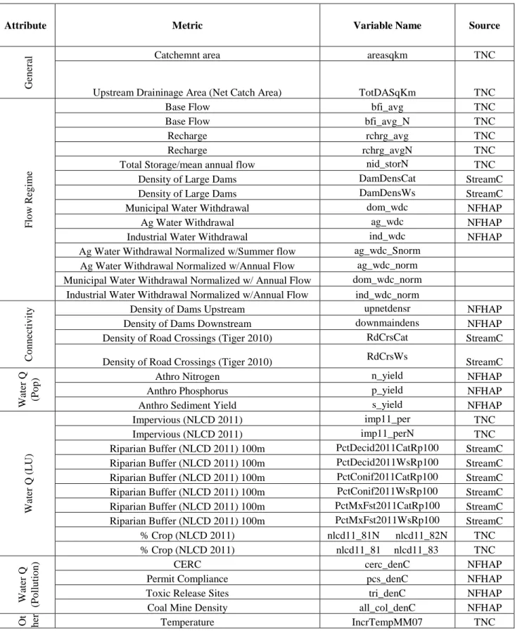
Table 1A. Full list of predictors, showing each variable’s thematic grouping and the source for each data set.
Attribute Metric Variable Name Source
Gen
er
al Catchemnt area areasqkm TNC
Upstream Draininage Area (Net Catch Area) TotDASqKm TNC
Flo w R eg im e
Base Flow bfi_avg TNC
Base Flow bfi_avg_N TNC
Recharge rchrg_avg TNC
Recharge rchrg_avgN TNC
Total Storage/mean annual flow nid_storN TNC
Density of Large Dams DamDensCat StreamC
Density of Large Dams DamDensWs StreamC
Municipal Water Withdrawal dom_wdc NFHAP
Ag Water Withdrawal ag_wdc NFHAP
Industrial Water Withdrawal ind_wdc NFHAP
Ag Water Withdrawal Normalized w/Summer flow ag_wdc_Snorm Ag Water Withdrawal Normalized w/Annual Flow ag_wdc_norm Municipal Water Withdrawal Normalized w/ Annual Flow dom_wdc_norm
Industrial Water Withdrawal Normalized w/Annual Flow ind_wdc_norm
C o n n ec tiv
ity Density of Dams Upstream upnetdensr NFHAP
Density of Dams Downstream downmaindens NFHAP
Density of Road Crossings (Tiger 2010) RdCrsCat StreamC
Density of Road Crossings (Tiger 2010) RdCrsWs StreamC
W
ater
Q
(Po
p
) Athro Nitrogen n_yield NFHAP
Anthro Phosphorus p_yield NFHAP
Anthro Sediment Yield s_yield NFHAP
W
ater
Q
(L
U)
Impervious (NLCD 2011) imp11_per TNC
Impervious (NLCD 2011) imp11_perN TNC
Riparian Buffer (NLCD 2011) 100m PctDecid2011CatRp100 StreamC Riparian Buffer (NLCD 2011) 100m PctDecid2011WsRp100 StreamC Riparian Buffer (NLCD 2011) 100m PctConif2011CatRp100 StreamC Riparian Buffer (NLCD 2011) 100m PctConif2011WsRp100 StreamC Riparian Buffer (NLCD 2011) 100m PctMxFst2011CatRp100 StreamC Riparian Buffer (NLCD 2011) 100m PctMxFst2011WsRp100 StreamC
% Crop (NLCD 2011) nlcd11_81N nlcd11_82N TNC
% Crop (NLCD 2011) nlcd11_81 nlcd11_83 TNC
W ater Q (Po llu tio n
) CERC cerc_denC NFHAP
Permit Compliance pcs_denC NFHAP
Toxic Release Sites tri_denC NFHAP
Coal Mine Density all_col_denC NFHAP
Temperature IncrTempMM08 TNC
Elevation elevcm_avg TNC
Elevation elevcm_avgN TNC
Slope slope_avg TNC
Slope slope_avgN TNC
R-factor rf30_avg TNC
R-factor rf30_avgN TNC
K-factor kfact_avg TNC
K-factor kfact_avgN TNC
Sand sand_avg TNC
Sand sand_avgN TNC
Silt silt_avg TNC
Silt silt_avgN TNC
L
an
d
sca
p
e
C
o
n
d
itio
n Percent Agricultural Land within ARA (HUC 8) Perc_Ag_HUC8
Percent Natural Land within ARA (HUC 8) Perc_Nat_HUC8 Percent Impervious Surface within ARA (HUC 8) Perc_Imp_HUC8
Percent Agricultural Land within ARA Perc_Ag
Percent Natural Land within ARA Perc_Nat