On the Arrow of Spacetime

On the arrow of spacetime

Alexandre Harvey-Tremblay1*

1 _{Independent researcher}

* Correspondence: [email protected]

Version November 20, 2018 submitted to Preprints

Abstract: Consistent with special relativity and statistical physics, here we construct a partition

1

function of space-time events. The union of these two theories resolves longstanding problems

2

regarding time. We will argue that it augments the standard description of time given by the

3

(non-relativistic) arrow of time to one able to describe the past, the present and the future in a manner

4

consistent with our macroscopic experience of such. First, using Fermi-Dirac statistics, we find

5

that the system essentially describes a "waterfall" of space-time events. This "waterfall" recedes in

6

space-time at the speed of light towards the direction of the future as it "floods" local space with

7

events that it depletes from the past. In this union, an observerOwill perceive two horizons that

8

can be interpreted as hiding events behind them. The first is an event horizon and its entropy hides

9

events in the regions thatOcannot see. The second is a time horizon, and its entropy "shields" events

10

fromO’s causal influence. As only past events are "shielded" and not future events, an asymmetry in

11

time is thus created. Finally, future events are hidden by an entropy prohibitingOfrom knowing the

12

future before the present catches on.

13

Keywords:Statistical Physics; Special Relativity; Arrow of Time

14

1. Introduction 15

1.1. Time

16

The connection between time in statistical physics and time in special relativity are both well

17

established (Popper [1], Layzer [2], Davies [3], Zeh and Page [44], Callender [5], Price [6], Landsberg

18

[7], Halliwellet al.[8], Carroll [9]). On the one hand, we have the statistical emergence of a macroscopic

19

arrow of time, and on the other, we have a causal relationship between space-time events limited by

20

the speed of light. As most other theories consider time to be little more than some reversible variable,

21

the claims made regarding time by these two theories pack quite a lot of heat (figuratively). Thus,

22

to further investigate the nature of time, a promising avenue might be to ask: what about time in

23

"statistical physics∪special relativity" — is it possible to combine causality (in the sense given by

24

special relativity) with the arrow of time? As it turns out, in doing so (achieving the combination) we

25

are rewarded with quite a lot of insight. First, let’s clarify the motivation for this union.

26

1.2. Problem 1: The direction of time

27

We recall the well-known thought experiment in which Maxwell’s demon (Maxwell [10], Knott

28

[11], Thomson [12], Leff and Rex [13]) consumes good information to return a macroscopic system

29

to some initial low-entropy state. An observer might naively conclude that the (macroscopic) arrow

30

of time (Weinert [14]) is reversed, but inspection of the global system reveals that Maxwell’s demon

31

produced entropy in amounts at least equal to the information consumed (Szilard [15], Landauer

32

[16], Bennett [17]).

33

Taking the universe to be the global system, and sub-systems to be local, equivalent thought

34

experiments can be produced. Borrowing terms from special relativity, we might say that the arrow of

35

time holds globally, but not locally. Gotcha! A global property in a non-relativistic theory is bound to

36

violate causality.

37

Or as George F R Ellis (Ellis [18]) states:

38

"The arrow of time locality issue: If there is a purely local process for determining the

39

arrow of time, why does it give the same result everywhere? [...] Local determination has

40

to arbitrarily choose one of the two directions of time as the positive direction indicating

41

the future; but as this decision is made locally, there is no reason whatever why it should

42

be consistent globally. If it emerges locally, opposite arrows may be expected to occur in

43

different places."

44

Resolving this issue is, of course, an interesting result of the model. In the model, the arrow of

45

space-time cannot be reversed by Maxwell’s demon, even locally, because the space-like entropy of the

46

sub-system, associated with the system’s past, grows throughout the cycle proportionally to the speed

47

of light. The causal influence of the system (which propagates at the speed of light in all directions), is,

48

in this model, the macroscopic system that would need to be reversed by Maxwell’s demon to reverse

49

the arrow of time. Thus, Maxwell’s demon cannot succeed unless it violates the speed of light.

50

1.3. Problem 2: Macroscopic time

51

If we were to only rely on time-symmetric differential equations (e.g. classical mechanics, unitary

52

evolution, etc.), there would be no meaningful difference between the past, the present, and the future.

53

Basically, time would be a point on a line and we could solve our equations as far into the future or

54

into the past as we wanted. This is quite far from our day-to-day experience of time.

55

Consistent with our macroscopic experience of time, the arrow of time improves the connection

56

between "time in the equations" and "time in real life" by giving it a direction favored by entropy. This

57

is better, but, as we will argue, not yet complete.

58

We will now scope our work by formulating some contemplation questions to elucidate what is

59

missing from the arrow of time, along with some leading questions to guide the discussion towards

60

the solution presented in this paper. Let’s start with two questions specifically related to the arrow of

61

time:

62

1. It is very unusual in science to have a quantity which sets the direction of another, but whose

63

magnitudes are not proportional. For instance, we can imagine an experiment which attains

64

thermodynamic equilibrium very quickly (e.g. an explosion), and one which takes a long time

65

(e.g. Earth’s core cooling off to room temperature). But in each case, the clocks are ticking at the

66

same rate. Why is the rate of passage of time not proportional to the magnitude of the arrow of

67

time, if its direction is correlated to it?

68

2. Special relativity sets the magnitude for the time evolution of an observerOin its own frame of

69

reference to be proportional to the speed of light. Leading question: Why is the direction of time

70

set by statistical physics, but its magnitude is set by special relativity, two seemingly unrelated

71

theories?

72

Furthermore, there is a noticeable difference between the past, the present, and the future that is

73

not captured by the arrow of time. An image that I like to use is that of an observer regretting the past,

74

worrying about the future, and acting (or failing to act) in the present. Consistent with causality,O 75

ought not to experience the other permutations, such as regretting the future or worrying about the

76

past.

77

Or, again, as George F R Ellis (Ellis [18]) states:

78

"As the nature of existence is different in the past and in the future - Becoming has meaning.

79

Different ontologies apply in the past and future, as well as different epistemologies"

80

With this image in mind, a further series of questions arises:

81

1. SupposeOgoes bird watching. Say the birds are observed for 20 years byO. ThenOshould

82

know a lot more about those birds today thanO did 20 years ago. O’s conclusion that time

has passed is evidenced by the existence of a "log of observations" maintained byO, and not

84

so much on the fact that the birds of today are ever so slightly closer to final cosmological

85

thermodynamic equilibrium than the birds of 20 years ago. Let’s emphasize the dichotomy:

86

the arrow of time points towards higher entropy (more hidden information), butOconcluded

87

that time moves forward by building up a log of events (gaining information). IsOmaking a

88

mistake by using a log of events to conclude as to the passage of time, instead of estimating the

89

system’s overall entropy as per the arrow of time? As George F R Ellis puts it, "we are aware of

90

the flow of time because of the existence of records of the past" (Ellis [18]). Leading question: Is

91

O’s construction of a log of events contributing to increasing the entropy of the system? What if

92

O’s log is complete (it lists all space-time events) — in this case, isO’s behavior of producing

93

information by increasing entropy the opposite of Maxwell’s demon? Perhaps it is "Maxwell’s

94

angel"? (Touchette and Lloyd [19], Parrondoet al.[20])?

95

2. Generally, if the universe started from a low entropy Big Bang and is evolving into a high entropy

96

state and that entropy is associated with a loss of information, what sort of compensation is there

97

to offset this loss? Leading question: Can the information gained by observing a system over time

98

be accumulated and is it enough to offset the information lost by the action of the arrow of time?

99

Can a statistical system aware of events reconcile both notions? From Landauer’s aphorism,

100

since "information is physical" (Landaueret al.[21]) where and how would his information be

101

stored(Gooldet al.[22], Streltsovet al.[23], Adessoet al.[24])?

102

3. Why is the causal connection between past, present and future asymmetric (Halliwellet al.[8])?

103

For example,Oopens the fridge and notices that there is milk in it.Owonders why the milk

104

is there. It would make no sense to appeal to the future to justify the presence of milk in the

105

present. Thus saying, "the milk is in the fridge becauseOwill drink it tomorrow and therefore

106

it must be here today forOto be able to drink it tomorrow — that’s why it is there!" makes no

107

sense becauseOcould simply elect not to drink the milk and the milk will still be in the fridge

108

today. It’s similar to how some people feel absolutely certain that they will win the lottery at the

109

next draw, and thus will buy a ticket today in an attempt to set up the present to be as consistent

110

as possible with the anticipated future winnings, only to witness the attempt fail. However, the

111

reverse explanation easily makes sense: the milk is in the fridge today becauseObought it at

112

the supermarket yesterday and put it in the fridge this morning. Why does the "algorithmic

113

reconstruction" of the past based on present evidence work, but the same reconstruction fails

114

when applied to the future? Using purely time-symmetric differential equations we would get a

115

different story: the present would fix both the past and the future! We could even appeal to the

116

future to justify the present. The "arrow of causality" that we experience fails to emerge from

117

exactly solvable time-symmetric differential equations.

118

4. FromO’s present, the future appears to have multiple outcomes that could occur (e.g:Ocould

119

elect to drink or not to drink the milk — we won’t know until tomorrow) (Eddington [25]).

120

Leading question: Is there an entropy that we could have missed, but is nonetheless associated

121

withO’s possible futures that somehow gets reduced asOtravels forward in time, as the present

122

unravels? Does this entropy prohibitO’s knowledge about the future?

123

Combining special relativity with statistical physics will allow us to account for the past, the

124

present, and the future as three distinct regimes of time in a manner consistent with experience and

125

with the points raised in these questions. Let us now describe in greater detail how this will be done.

126

1.4. Outline

127

We consider two approaches that we could use to combine statistical physics with special relativity.

128

One approach is to make the standard quantities of statistical physics (e.g., entropy, temperature)

129

Lorentz-invariant. Using this methodology, we are rewarded with a frame-independent partition

130

function. The result of this approach yields non-relativistic statistical physics in the limitc→∞. This

131

is the approach taken by Giorgio Kaniadakis (Kaniadakis [26]).

Another approach is to seek a statistical ensemble whose macroscopic description relates to

133

special relativity. As special relativity is concerned with the relationship between space-time events,

134

this approach elects to make special relativity emergent (via an equation of state) from a statistical

135

ensemble of space-time events. In this case, special relativity is an emergent behavior caused by the

136

random statistics of space-time events.

137

The latter approach is the one that will be taken in this paper. Not only does it paint a seductive

138

picture of time and space, but it is also attractive because of its ability to explain the nature of

139

macroscopic time.

140

Using Fermi-Dirac statistics over an ensemble of space-time events, we show (section3.3) that the

141

space-time counterpart to the arrow of time is a "waterfall of events". Like the arrow of time, it too has

142

a direction: it recedes in space-time at the speed of light towards the direction of the future (section

143

3.4). Furthermore, as it recedes, the waterfall of events floods the present with immediate events and

144

depletes the past of events. As we will see, this behavior connects to the three regimes of time (section

145

3.7and4).

146

1.5. Improvements upon prior work

147

The prior work closest to ours are probably the works of (Jacobson [27]) and the works of (Verlinde

148

[28]), in which general relativity, classical gravity and the law of inertia are derived from statistical

149

physics. To derive the law of inertia, Verlinde [28] considers a length conjugated with an entropic

150

force, then under injection of the Unruh temperature, finds F = ma. To derive general relativity,

151

Jacobson [27] considers an area conjugated with an entropic surface tension, then under multiple

152

reasonable assumptions (Raychaud-Huri equation, local energy conservation, Null-horizons, etc.)

153

recovers Einstein’s fields equations. Thus, a pattern is beginning to emerge in the literature in which

154

some laws of physics are consistent when formulated as having their origin in entropy. Here, we

155

extend their work by placing time on equal entropic footing as these authors have done for length and

156

area. Specifically, we will consider a time conjugated to an entropic power in the context of emergent

157

special relativity.

158

2. A statistical ensemble of events 159

Our goal for this section will be to recover the "features" of special relativity strictly using the

160

facilities of statistical physics. In this case, we would say that special relativity is an emergent property

161

of the constructed statistical ensemble. Even the speed of light will not be taken as an axiom, but it will

162

instead be a property emergent from the construction. How will we do that? First, we have to interpret

163

the speed of light as a tool to hide information. Specifically, the speed of light hides information

164

regarding events whose intervals to the observer are space-like. Interpreted as such, we can then use

165

the entropy in statistical physics to achieve the same purpose as the speed of light (hide information),

166

provided that we "place" the entropy appropriately in the system.

167

For instance, we can imagine an observerOwhose event horizon is defined by the usual light cone

168

of special relativity. We can then describe this light cone entirely using notions of statistical physics by

169

analyzing the number of configurations of events outside the horizon and associating it to an entropy.

170

We deduce that, to prevent faster-than-light communication, all possible configurations of events

171

outside the event horizon must be of maximal entropy (e.g., equally likely within the priors) so as to

172

be void of information from the perspective ofO. This entropy thus hides events outside the horizon.

173

Attributing an entropy to events separated by a horizon in order to connect to thermodynamics has

174

been done since at least 1973 by J.D. Bekenstein (Bekenstein [29]). Furthermore, from G. W. Gibbons

175

and S. W. Hawking’s 1977 article (Gibbons and Hawking [30]), I quote:

176

"An observer in these models will have an event horizon whose area can be interpreted as

177

the entropy or lack of information of the observer about the regions which he cannot see."

The part missing from the picture of time, we suggest, is to apply the same line of reasoning to

179

configurations of future events. We ask, how many configurations of future events are compatible

180

with the present state? First, we pose this assumption: since the present is caused by the past (not the

181

future), there exists strictly more than one configuration of future states compatible with the current

182

present. The use of the quantifierstrictly more than oneis important here as if it were not the case (i.e.

183

there is only one configuration of future events), then the present would be "caused/determined"

184

by the future as much as by the past. Causality would be time-symmetric. This assumption is the

185

foundation of the past/future asymmetry we recover in this union. For instance, an observer trying to

186

pre-solve time-symmetric exact equations will, due to this entropy, fail to predict which of the possible

187

futures will actually occur. However, once the future has become present, solving those same equations

188

backward will go as expected. We, of course, assume that an observer has no prior knowledge of his

189

future (no foresight). Thus, configurations of compatible future events must be of maximum entropy

190

otherwise information about the future would be available toO(foresight).

191

Using this strategy, we can obtain a system of statistical physics over space-time events that

192

follows the rules of special relativity.

193

Other emergent features we would like to have (briefly listed and to be expanded in section3)

194

are: a) recovering the fundamental equation of special relativity, linking time to spacedx=cdtfrom

195

the equation of state; b) having the entropy at the horizon corresponding to the Bekenstein-Hawking

196

entropyS=kBA/(4L2p); c) having the speed of light defined as an emergent property of the system,

197

which is constant and that cannot be exceeded; d) connecting time-like separated events with a

198

"time-like entropy" and space-like separated events with a "space-like entropy"; e) having an emergent

199

arrow of space-time that generalizes the arrow of time to special relativity. This list of requirements

200

might sound like the statistical system would be complicated to describe, but all it takes is maximizing

201

the entropy on average t (system age) and x (system size), and everything we need will emerge out of

202

it. Let’s get started.

203

2.1. Background

204

We suppose a 3+1 space-timeM4in spherical coordinates{r,θ,φ,t}. Under isotropic assumptions

205

{dθ =0,dφ= 0}the space-time is simplified to a 1+1 space-timeMwith coordinates{r,t}, and it

206

enforces the constraint thatr∈R≥0. Additionally, we pose thatt=0 is the origin of the system, and 207

thust∈_R≥0. Finally, we denote an observer byO. 208

2.2. Events

209

LetQbe the set of events inM. We define the functionsrandtas mapping each eventq∈Qto

210

its space-time position inMas:

211

r:Q→R≥0[meters] (1)

t:Q→R≥0[seconds] (2)

2.3. Macroscopic system of events

212

We consider a macroscopic system defined for a set of eventsQand two macroscopic quantities

213

(the priors): an average event-timet∈ R≥0, and an average event-distancer ∈ R≥0. We offer two 214

justifications for these priors.

215

Mathematical justification: First, to treat the events as microscopic elements of a macroscopic

216

system of statistical physics, we are required to take the averages of the quantitiesr(q)andt(q)as the

217

priorsrandtof the macroscopic system when we derive the Gibbs ensemble under an appropriate

218

notion of equilibrium. This is analogous to taking the average energyEas the macroscopic description

219

of a system microscopically described by energy levelsE(q), under the assumptions of thermodynamic

equilibrium. Another example would be taking an average volumeVover the possible volumesV(q),

221

etc..

222

Physical justification:

223

Math notwithstanding, this is a physics paper and thus, the priors must be physically justified.

224

First, consider that in usual special relativity, the observer is conceptually understood to be the origin of

225

the system, and as such its light cone extends to infinity both in the past and in the future. Empirically

226

however, this is not the quite the case. The past light cone of any observer that we find in nature (e.g.

227

of real observers) does not extend to infinity in the past, but terminates at the Big Bang. Thus, such

228

real observers come with a prior light cone of a certain size and age. For instance, the light cone of a

229

present-day observer will come with priors regarding the size of its light cone and the origin is not the

230

observer, but instead coincide with the Big Bang at(0, 0). In this context, the priors are essentially the

231

initial conditions regarding the size of the light cone of real observers respective to the origin of the

232

system.

233

This accounts for the priors being non-null, but it doesn’t yet answer why these priors are average

234

values instead of exact values. To address this, let us first give a classical example, then we will justify

235

it more fundamentally.

236

1. If we were to request five hundred independent measurements of the size of the present-day

237

particle horizon, we would likely get five hundred slightly different values. Thus, in the case

238

where the values of the priors are empirically derived, we would end up with an average

239

experimental value with some expected fluctuations over the set of measurements. This argument

240

is purely classical, but we can make it fundamental by evoking notions of quantum mechanics.

241

2. In the formalism of special relativity, the observer O is point-like and the size of the light

242

cone expanding away fromOcan be measured to arbitrary precision. Ergo, the theory is not

243

aware of the quantum mechanical restrictions on the precision of measurements. Assume that

244

instead of being point-like,Ois of a size described by its Compton wavelength. In this case,

245

since the observer is not point-like, the dimension of the light cone expanding from it can no

246

longer be considered arbitrarily precisely, even fundamentally. Thus, in this context we would

247

expect that any attempt at measuring the dimensions the surface of the light cone will exhibit a

248

certain statistical character preventing its measurement to a precision exceeding the Compton

249

wavelength of the object of reference.

250

Referencing the Compton wavelength has previously and successfully been done before in an

251

analogous context regarding the Black Hole information paradox, general relativity, black hole entropy

252

and statistical physics in (Hawking [31]) and to entropy over positional information in (Verlinde [28]).

253

Here, we will soon recover the Compton wavelength explicitly from the equation of state (equation

254

25), and by doing so we will be able to show that the system exactly connects to a gamut of related

255

physical laws including the law of inertia, the Unruh temperature, the Bekenstein-Hawking entropy

256

(equation27). For these reasons, interpreting the Compton wavelength as a limitation on the size of the

257

observer does appear to be the proper physical relation to limit the precision of the point-like observer

258

in the context of statistical physics∪special relativity, as it will make the union nicely fit into many

259

prior results of physics.

260

2.4. Gibbs ensemble of events

261

Under the principle of maximum entropy, we seek the probability distributionρ:Q → {p ∈

262

R|0≤p≤1}and∑q∈Qρ(q) =1 which maximizes the entropyS:

263

S=−kB

∑

q∈Q

ρ(q)lnρ(q) (3)

and subject to the priorstandr

t=

∑

q∈Q

ρ(q)t(q) (4)

r=

∑

q∈Q

ρ(q)r(q) (5)

We maximize the entropy using the well-known method of the Lagrange multipliers.

265

L= −kB

∑

q∈Q

ρ(q)lnρ(q)

!

+λ0

∑

q∈Q

ρ(q)−1

!

+λ1

∑

q∈Q

ρ(q)t(q)−t

!

+λ2

∑

q∈Q

ρ(q)r(q)−r

!

(6)

MaximizingLwith respect toρ(q)is done by taking its derivative and posing it equal to zero:

266

∂L

∂ρ(q) =−kBlnρ(q)−kB+λ0+λ1t(q) +λ2r(q) =0 (7) Solving forρ(q)we obtain:

267

ρ(q) =exp

₋

kB+λ0+λ1t(q) +λ2r(q)

kB

(8)

From the constraint 1=_∑q∈Qρ(q), we can find the value forλ0: 268

1=

∑

q∈Q

ρ(q) (9)

=

∑

q∈Q

exp

_−k

B+λ0+λ1t(q) +λ2r(q)

kB

(10)

=exp

₋

kB+λ0

kB

∑

q∈Q

exp(λ1t(q) +λ2r(q)) (11)

We define the partition functionZto be

269

Z:=

∑

q∈Q

exp(λ1t(q) +λ2r(q)) (12)

Then, we rewriteρ(q)usingZ, we poseλ1:=1/t0andλ2:=−1/r0and we obtain the probability 270

distribution:

271

ρ(q) = 1 Zexp

1 t0t

(q)− 1 r0r

(q)

(13)

where 1/t0 with units [1/(seconds)] and −1/r0 with units [1/(meters)] are the Lagrange 272

multipliers (a justification for the choice of signs will be provided after the results in section4.3).

273

Finally, we obtain the equation of state:

dS=−kB t0

dt+kB r0

dr (14)

which represents the macroscopic evolution of the system, and wherekBis Boltzmann’s constant.

275

The reason why the author has elected to produce the explicit derivation of the Gibbs ensemble for

276

this system is to show clearly that a Gibbs ensemble of statistical physics (such as the one here) can

277

legitimately be constructed without the introduction of an emergent temperature (as a Lagrange

278

multiplier) associated with thermodynamic equilibrium. Thus, the present system holds outside of

279

thermodynamic equilibrium, although another type of equilibrium is required on the 1/t0and−1/r0 280

Lagrange multipliers. Perhaps the name "tempo-dynamic equilibrium" is fitting? In this case, the

281

Lagrange multipliers 1/t0and−1/r0would be the "tempo-ture" of the system. 282

Definition: We will define "light-like" entropy, "time-like" entropy, and "space-like" entropy. Each

283

is obtained by solvingdSin (14) but under different conditions. The first refers todSat tempo-dynamic

284

equilibrium (1/t0dt=1/r0dr). The second refers to the case where 1/t0dt>1/r0dr, and the third to 285

1/t0dt<1/r0dr. 286

Remark: Since the universe is not at uniform temperature, cosmological thermodynamics has

287

been focused on the study of event horizons, which admits temperatures (Hawking [31], Unruh [32]).

288

Resisting the temptation to include an averageE, and thus relaxing the requirement that the system be

289

at thermodynamic equilibrium with a uniform temperaturetwas a key insight which opened the door

290

to apply statistical physics away from the surface of horizons, and within the volume of the enclosing

291

surface. This is possible at "tempo-dynamic" equilibrium. As we will see, instead of admitting

292

a uniform temperature (as in the thermodynamic equilibrium case), a system at tempo-dynamic

293

equilibrium admits a uniform maximum speed.

294

3. Results 295

3.1. Tempo-dynamic quantities

296

Consistent with the standard interpretation of statistical physics, physical quantities that are

297

extensive are conjugated with an intensive quantity. For instance the volumeVin statistical physics is

298

extensive and combining the volume of two sub-systems increases the volume by the sumV1+V2=V 299

(extensive), but the pressure is not added: p1=p2=p(intensive). Experimentally, two systems with 300

different pressuresp1 6= p2can be joined together, but this breaks the thermodynamic equilibrium 301

until the pressures equalize. Likewise, a process which consumest1seconds followed by a process 302

consumingt2seconds consumes a total oft1+t2 = tseconds (extensive) while its conjugate time 303

is intensive (1/t0is a constant Lagrange multiplier). Same goes with position: adding two meters 304

end-to-end doubles the length (extensive) whereas its conjugate position, as it is a Lagrange multiplier,

305

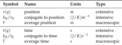
remains the same (intensive). These quantities are summarized in the Table (1).

306

Table 1.The relevant tempo-dynamic quantities

Symbol Name Units Type

r(q) position m extensive

kB/r0 conjugate to position (J/K)m−1 intensive

r average position m macroscopic

t(q) time s extensive

kB/t0 conjugate to time (J/K)s−1 intensive

A

O

B

c:

=

r

0

/

t

r

t

Figure 1.A tempo-dynamic cycle in time and space is reminiscent of the structure of a light cone in special relativity.

3.2. Tempo-dynamic cycles in time and space

307

Equation (14), as it references a timetand a distancer, imposes requirements on the entropy of

308

the system as the light cone expands. To investigate the behavior, let’s us take Figure (1) as an example

309

of a simple tempo-dynamic cycle involving time and space. The cycle is reminiscent of a light cone,

310

but it makes additional claims about the entropy. The transitions along the cycle are:

311

1. isospatial process: While transiting fromOtoAand by keeping the distance constant (dr=0),

312

the system decreases its entropy :dS/dt=−kB/t0. 313

2. isotemporal process: While transiting fromAtoBand by keeping the time constant (dt=0), the

314

system increases its entropy :dS/dL=kB/r0. 315

3. isentropic process: While transiting fromBtoOand by keeping the entropy constant (dS=0),

316

the system’s size increases at a characteristic constant speed :dr/dt=r0/t0. 317

3.3. Fermi-Dirac statistics of events

318

We consider that an event can occur at most once (whatever happens to Schrödinger’s cat, for sure,

319

it doesn’t die twice), and thus we will use Fermi-Dirac statistics to study the occupancy distribution of

320

events. In the case of (14), its Fermi-Dirac distribution under the assumption thatµ=0 is:

321

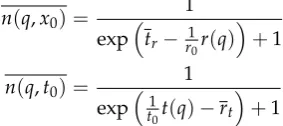
n(q,t0,r0) =

1

exp_t1

0t(q)−

1

r0r(q)

+1

(15)

To better understand what is going on with this equation (Fermi-Dirac statistics over space and

322

time quantities), it helps to first illustrate the Fermi-Dirac statistics of bothr(q)andt(q)in isolation.

323

Therefore, consider these Fermi-Dirac distributions applicable tor(q)andt(q), respectively. In each

324

case, one of the two quantities has been made constant for the purposes of simplification. The two

325

distributions (16) and (17) are illustrated in Figure2a and2b, respectively. The equations are:

326

n(q,x0) = 1

exptr−_r1₀r(q)

+1

(16)

n(q,t0) = 1

exp_t1

0t(q)−rt

+1 (17)

Now we are ready to investigate the Fermi-Dirac distribution given in (15) as illustrated in Figure

327

3.

t

r

/

t

<

n

>

Fermi

-

Dirac

a

)

Occupancy of r for

t

r

t

/

r

<

n

>

Fermi

-

Dirac

b

)

Occupancy of t for

r

t

r

/

t

<

n

>

Bose

-

Einstein

c

)

Occupancy of r for

t

r

t

/

r

<

n

>

Bose

-

Einstein

d

)

Occupancy of t for

r

Figure 2. a)Fermi-Dirac statistics (equation16) over the occupancy of space-time events in relation to their distance fromr=0, while holding the average timetrconstant. The shape of the curve is of the

familiar shape and direction as the well-known distribution applicable to energy levels. The slope at tris correlated to the value ofr0and is analogous tokBTin the case of energy levels.b)Fermi-Dirac

statistics (equation17) over the occupancy of space-time events in relation to their timet, while holding the average positionrtconstant. The shape is the same as the previous case, but its direction is mirrored

at thertline.c)andd): We argue at the end of section3.3that Bose-Einstein statistics are inapplicable

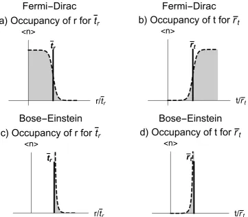
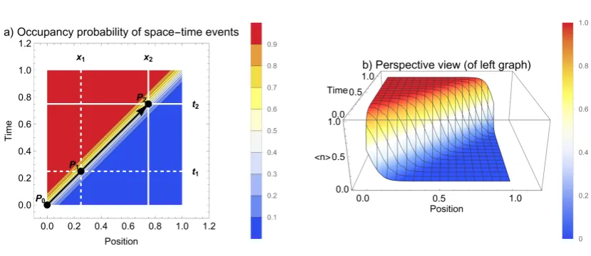
Figure 3. Fermi-Dirac statistics over the occupancy of space-time events (equation 15and with

µ=0). Red means an occupancy rate of 100%, whereas blue means 0% (and with rainbow colors for intermediate values).a)The slicest1andt2have the same shape as Figure2a. The slicesx1andx2 have the same shape as Figure2b. As the system goes fromP1toP2, occupied past states are depleted as distance states become saturated. The slope of the line fromP1toP2is the speed of light, associated with the ratio of the tempo-ture of the system.b)The image on the right is a perspective view of the image on the left.

Description: For the future, the occupancy rate of events is saturated (future events are upcoming).

329

For the past, the occupancy rate of events is depleted (past events are gone). An observerOevolving

330

fromP1toP2will, inO’s present, experience a transfer in the saturation of the occupancy of future 331

events to a saturation in the occupancy of events in space. This is the point at which we introduce the

332

analogy of the waterfall of events flooding space. Along withO, this "waterfall of events" recedes in

333

space-time at the speed of light towards the direction of the future as it "floods" local space with events.

334

Ois prohibited by entropy from knowing future events until the waterfall recedes appropriately. Past

335

events are depleted from the system following the passage of the waterfall. SinceOsees no occupied

336

past events, O’s future in space-time lies in the forward time direction, and the waterfall recedes

337

towards the future. Let’s prove this direction in the next section, and then return to this discussion in

338

section4.

339

A note on Bose-Einstein statistics: We believe that Bose-Einstein statistics (BE) are inappropriate

340

for the description of events for the following reasons:

341

1. Repeating an event that has already occurred (if such a thing is even possible) is not expected

342

to contribute to the information of the system. For instance, re-measuring Schrödinger’s cat

343

multiple times over does not make it more or less dead than it already is (if dead, or alive

344

otherwise). Generally, performing a quantum measurement on a quantum system already in an

345

eigenstate leaves the system unchanged. Thus, we would expect events to be registered only

346

when they first occur; that is to say, their informational contribution occurs at most once.

347

2. The occupancy rate of events described by Bose-Einstein statistics falls quickly away from the

348

observer and reaches near-zero well before reaching the event horizon of the light cone. Thus, the

349

argument that the occupancy rate of events represents those events that are causally connected

350

to the observer, does not hold under Bose-Einstein statistics.

351

3. Under Bose-Einstein statistics, future states are depleted and both the past and the inside of

352

the event horizon are undefined. Figure (2c) and (2d) show that Bose-Einstein statistics are

only defined for the future and for outside of the event horizon. This is inconsistent with event

354

horizons in special relativity.

355

4. Under Bose-Einstein statistics, the present occurs at a mathematical singularity which is,

356

obviously, undesirable.

357

3.4. Arrow of time

358

Our goal here is to prove that the waterfall recedes in the direction of the future.

359

Let us first investigate the production of entropy over time in (14). To do so, we divide each side

360

of (14) bydtthen multiply it byr0/kB. We obtain:

361

r0

kB

dS dt =

r0

t0 −dr

dt (18)

First, we note that as both−1/r0and 1/t0 are Lagrange multipliers, then bothr0 andt0are 362

uniform in the system. The ratior0/t0is a speed[meters/seconds]and is also uniform. 363

Second, we note that (18) represents an inflection point in the production of entropy in the system

364

atdS/dt=0. Specifically, whendS/dt<0, the entropy of the system decreases as a whole, which

365

is prohibited by the second law of thermodynamics. This occurs if the macroscopic system (randt)

366

shrinks (dr/dt<0) or grows slower than the ratior0/t0. 367

Discussion: We now conclude, based on the two points mentioned, that the arrow of time points

368

towards the future of the macroscopic system whose growth in space-time is prohibited by the second

369

law of thermodynamics from being less than the ratio of the tempo-ture. Now that we know the

370

minimum growth rate, we might wonder, what, if anything, prevents the system from exceeding the

371

ratio? Answer: the observer does not see events beyond the horizon because the occupancy probability,

372

given by Fermi-Dirac statistics, sharply drops to zero at the horizon. This limits the growth rate of the

373

system as perceived byOto the ratio of its tempo-ture.

374

3.5. Recording the passage of time

375

We integrate equation (14). We get:

376

Z

dS=−kB t0

Z

dt+kB r0 Z

dr (19)

∆S=−kB t0∆t

+kB r0∆r

+C (20)

This relation leads to two inequalities:

377

0≤ −∆S≤ kB

t0∆t 0

≤∆S≤ kB

r0∆r (21)

The first, involving time, relates the minimum amount of information (−∆S) that must be acquired

378

to prove that time has passed by a certain amount∆t. It is interpreted in the sense that the passage of

379

time∆trequires the logging of an event−∆S. The second, involving space, relates an entropy (∆S)

380

to the minimum increase in the size of space∆rrequired to accommodate it. Let us now study this

381

behavior in more detail by constructing an (abstract) thermodynamic engine that converts time to

382

space.

383

3.6. Space-time engine

384

We will define a thermodynamic engine that converts time to space. The engine is comprised of

385

a detector and a tape. The engine can write one bit on the tape atr=0. It can also shift the tape to

the right by one increment∆r(in preparation to write the next bit). For purposes of idealization, we

387

consider that the engine never runs out of tape. Finally, and without loss of generality, it helps for the

388

purposes of the illustration to consider the more familiar case where the system is at thermodynamic

389

equilibrium. Thus, we pose thermodynamic equilibrium to the inequalities with these replacements:

390

kB/t0 := P/T where P is a power in [Joules/seconds], and kB/r0 := F/T where F is a force in 391

[Joules/meters], and whereTis a temperature in[Kelvins]. We get:

392

0≤ −∆S≤ P

T∆t 0≤∆S≤

F

T∆r (22)

To ease the abstraction, we can picture a concrete system sharing similar characteristics (with

393

some limitations), such as a seismograph tracing seismic data (collected over time) on a rolling tape

394

(stored in space). The cycles of the engine occur in parallel and are completed over a time period∆t.

395

Each cycle represents a logical step in the process (not chronological). They are:

396

1. Shifting the tape to the right by∆ris favored by entropy as it increases it by∆S. Thus, an entropic

397

forceFemerges which pulls on the tape. For this engine, we associate this increase in entropy to

398

an undefined memory address (∆S=kBln 2) which becomes available at position 0 of the tape

399

when it is shifted by∆r.

400

2. The detector clicks (it produces information). To register the click,∆tincreases as∆Sis decreased.

401

To pay the energy cost to decrease the entropy, the detector draws a powerPfrom the engine

402

over the time period∆t.

403

3. Finally, the engine writes the bit associated with the click in the undefined memory address of

404

the tape. This reclaims the energy of the shift (F∆r) that produced the entropy and instead makes

405

it available to power the detector (P∆t).

406

This engine has an interesting property: the further along the tape one looks, the further back in

407

time the information on the tape refers to. At tempo-dynamic equilibrium, the tape is shifted at the

408

speed of light towards the right, and its farthest bit refers to the very first thing that has been recorded.

409

Ergo, this engine produces a light cone.

410

3.7. Gamut of related laws

411

Let us calculate the entropy at the horizon for the system then we will be in a good position to

412

discuss these results.

413

We can show that the entropy at the horizon is no greater than the Bekenstein-Hawking entropy

414

(Bekenstein [29], Hawking [31], Susskind [33]). To derive it, we must be consistent with the conditions

415

permitting the derivation of the Bekenstein-Hawking entropy in the first place: event horizons have a

416

temperature (Hawking [31], Unruh [32]).

417

First, we pose dt = 0. Then, the first step of the proof will involve taking the system at

418

tempo-dynamic equilibrium (14) and making it into a system that is also at thermodynamic equilibrium.

419

To do so, we must insert a temperature into the system while keeping in mind that 1/r0is a Lagrange 420

multiplier and, thus, is uniform at equilibrium. Preserving the units while injecting a temperature,

421

we pose the relationkB/r0 := F/T(whereFis a force in[Joules/meters]andTis a temperature in 422

[Kelvin]), and we get:

423

dS= F

Tdr (23)

For the system to be at thermodynamic equilibrium (and thus to admit a temperature), we are

424

looking for a temperature associated with black-body radiation and applicable to an object under the

425

action of a force. Within the context of special relativity, this is of course the Unruh effect (Unruh

[32], Fulling [34], Davies [35]), whose characteristic temperature is given byT:= (¯ha)/(2πkBc)and

427

applicable to an object undergoing accelerationF:=ma. Making the replacements intoF/T, we get

428

both the ratioF/TandTto remain uniform as required, and we obtain:

429

F

T =2πkB mc

¯

h (24)

Since the massmcan change, we have to insert the ratioF/TintoS = _TFr, then take the total

430

derivative ofS:

431

dS=2πkBmc

¯

h dr+2πkB rc

¯

hdm (25)

where ¯h/(mc)is the well-known reduced Compton wavelength. Here, the first term is acting as

432

the factor of proportionality between the entropy and the distance (Verlinde [28]). In the case ofdr,

433

we find that the Compton wavelength mediates the intensity of the fluctuations around the average

434

valuer, consistent with our justification of the priors in section2.3. We notice that the higher the mass,

435

the higher the entropy. Since the most massive object for a givenr(radius) is a black hole, we pose

436

r:=2Gm/c2(the Schwarzschild radius) as the upper limit on entropy. The black hole also has the

437

benefit of being isotropic with respect to its center, consistent with our assumptions in section (2.1). We

438

now use the Schwarzschild radius to replacerwithmwhere appropriate to simplify (25) to:

439

dS=8πkB

Gm ¯

hc dm (26)

After integrating, we getS=4πkBGm2/(hc¯ ) +C, whereCis an integration constant. Then, by

440

posingA:=4πr2s =16πG2m2/c4and using the Planck lengthLp:=

√ ¯

hG/c3_{, we get a boundary on} 441

the size of the entropy as:

442

S≤kB A

4L2

p

+C (27)

which is proportional to the surfaceAand includes the factor 1/4. This result serves as a sanity

443

check: The Bekenstein-Hawking entropy is recovered! Naturally, we interpret the surface as an event

444

horizon and the ratio of tempo-turer0/t0as the speed of light. 445

4. Discussion 446

We can now understand how, precisely, recording events connects to (and even produces) the

447

arrow of time. To investigate this, instead of considering the second law of thermodynamics as a

448

logically independent axiom, we will inject it into an equation of state in order to study its contribution

449

quantitatively. We recall the second law of thermodynamics which state that the entropy of a system

450

stays constant or increases (dS≥0), but never decreases. In the context of the arrow of time, we are

451

interested in the second law of thermodynamics as it pertains to time.

452

dS

dt ≥0 (28)

We can rewrite this inequality using a functionCas follows:

∂S ∂t

_V,N,E

=C whereC≥0 (29)

Formulated as such, the arrow of time is mathematically equivalent to (28), but in this format

454

it is more immediately recognizable as a candidate thermodynamic law. For instance, the laws of

455

thermodynamics regarding entropy, volume and particle number are often expressed as:

456

∂S ∂E

_V,N

= 1 T

∂S ∂V

_E,N

= p T

∂S ∂N

_E,V

=−µ

T (30)

To turn (29) into a valid thermodynamic law, it suffices to replace C with −P/T under an

457

appropriate equilibrium situation, wherePis an entropic power in[Joules/seconds]andT is the

458

temperature in[Kelvin]. Taking these laws, along with (29), we can summarize them into an equation

459

of state:

460

dE=TdS−pdV+µdN+Pdt (31)

where the last termPdtis responsible for enforcing the arrow of time explicitly within the equation

461

of state itself.

462

To make sense of this equation of state, it helps to imagine a quantum gas whose molecules are

463

under continuous measurements by the environment. First, recall that in the quantum case, the results

464

of measurements are intrinsically random and therefore to reverse the system, contrary to the classical

465

case, it is not sufficient to simply know, with infinite precision, the initial state of the air molecules (as

466

per Laplace’s demon). In the quantum case each random measurements produced by the environment

467

over time would have to be recorded in the degrees of freedom of the environment to make the history

468

of the system complete in the information theoretic sense.

469

A problem however arises while doing this. The memory requirements of the log of event will

470

outgrow any finite system, unless the system grows too. Why? Consider a gas at thermodynamic

471

equilibrium. The quantum molecules are continuously being measured by the environment even at

472

equilibrium and thus the system must store a perpetually growing log of events. To accommodate the

473

growing log, the system must somehow grow its memory proportionally to the rate at which events

474

are produced. This is why special relativity emerges as an entropic law in this context. Indeed growing,

475

at the speed of light, an event horizon (which bears an entropy) around the system guarantees that

476

the memory requirements for storing all such events as they occur in time are met. The entropy on

477

the surface of this event horizon is sufficient to make the system thermodynamically-reversible in

478

time, and thus the log of events is complete. From this, we are now ready to discuss how the past, the

479

present and the future emerges from these properties.

480

4.1. Three regimes of time

481

Reprising our discussion over the system’s qualitatively different description of the past, the

482

present, and the future, we now study the entropy dynamics of both time and distance in the context

483

of entropic special relativity. As concluded in section (3.7), when time is ignored, an observer perceives

484

the the space-like entropy to be the Bekenstein-Hawking entropy. However, the situation is different at

485

tempo-dynamic equilibrium when time is included. In this case, we find that the entropy reduction of

486

increasing thetquantity exactly compensates the entropy increase associated with increasing ther

487

quantity. From this, we would find that the observer, at tempo-dynamic equilibrium, always sees an

488

entropy of 0 in the present (plus an integration constant, to be neglected from the discussion). How do

489

we make sense of this result?

First we note that in the quantum case, unlike Laplace’s demon in the classical case, knowing the

491

initial conditions of the system is not sufficient to replay it. However, with both the initial conditions

492

and the log of events, we have enough information to replay the system from the beginning even

493

in the quantum case. As this information is sufficient to fix the present to a single solution, then

494

any additional information beyond it is therefore necessarily redundant which is why, inevitably, we

495

obtained the Bekenstein-Hawking entropy, as an upper bound on entropy, in this case.

496

The surface of the event horizon can be interpreted as keeping a record of all events relevant

497

toO’s present that have transpired since the Big Bang, in an manner complete in the information

498

theoretic sense such that the present state of the observer can be exactly recovered by replaying the log

499

from the initial conditions and under an appropriate quantum theory.

500

We describe each regime of macroscopic time as follows:

501

• Present: We associate light-like entropy with the uniquely determined present. As stated, the

502

present has an entropy of 0. It is uniquely determined by the initial conditions of the system

503

plus the log of random events that have occurred since the beginning of the system up to the

504

present time. As a result, the observer cannot be in a superposition of multiple presents and

505

consequently, we expect the observer to "measure" Schrödinger’s cat as either dead or alive, but

506

not as a superposition of both.

507

• Past: We associate space-like entropy with a trace of the past. As the waterfall recedes in

508

space-time, it leaves a trace of events in the degrees of freedom of space. An observer can, by

509

inspecting the trace, find evidence for a consistent past to account for the present. The horizon

510

produced by the depletion of past events under Fermi-Dirac statistics prohibitsOfrom going

511

backward or interacting with past events (Figure2b) directly. A similar horizon, also enforced by

512

state depletion, is found at the edge of the event horizon in space (Figure2a).

513

• Future: Finally, we associate time-like entropy with the future. The observer is prohibited from

514

peeking into its future (increasingtabove tempo-dynamic equilibrium) until it is imminent.

515

Indeed, an observer peeking into the future (without first waiting for the waterfall to recede

516

appropriately) will hit negative entropy (contradiction). The observer can hypothesize about

517

its possible futures, but the actual future is made final no sooner than in the present when the

518

entropy hits 0. This negative entropy prevents the macroscopic system from growing faster than

519

allowed by tempo-dynamic equilibrium.

520

So why do we think there is an entropy in the gas of the room I am in, for instance, if the entropy

521

of the present is allegedly zero? This is because I do not know all the bits of the log of events, thus,

522

I can successfully approximate the gas in the room as an entropic system. Partial knowledge of the

523

trace of events byOlimits the uniqueness of the reconstruction of the past achievable byObased on

524

the analysis of the trace, as it represents the number of logs of events that are compatible with the

525

observer’s unique present under partial knowledge of the log.

526

What about the arrow of time? This now accounts for only half of the story. The waterfall of

527

events, as it recedes in space-time, creates two arrows related to time. The first arrow is the familiar

528

one. The entropy associated with the degrees of freedom of space ((kB/r0)dr) increases as time moves 529

forward. The second arrow acts in the reverse direction on the degrees of freedom of time ((−kB/t0)dt). 530

With it, the entropy associated with time decreases as time moves forward because future possibilities

531

are consumed to create a present.

532

4.2. Falsifiable prediction

533

From equation (14), and preserving the units, we impose thermodynamic equilibrium on the

534

system with the replacementkB/t0:=P/TwherePis a power[Joules/seconds]andTis a temperature 535

[Kelvin]. By further posingdr=0. We get:

TdS=−Pdt (32) This equation predicts that an entropic power can be made to emerge if information is produced

537

(or consumed) over time and at constant temperature. This prediction regarding the possibility of an

538

emergence of an entropic power should be relatively easy to show experimentally.

539

4.3. Note on the signs of the Lagrange multipliers

540

The signs of the Lagrange multipliers were chosen for the following reasons: 1) Starting with

541

(14) and posingdS=0 we getdr=cdt(wherec:=r0/t0). This is the fundamental relation of special 542

relativity connecting space to time. Thus, the signs of the Lagrange multipliers must be opposite. 2) In

543

the derivation of the Bekenstein-Hawking entropy, we have usedF=ma, and notF=−ma. Thus, the

544

Lagrange multiplier of−1/r0must be negative. 3) The combination of reason one and two implies 545

that the sign of 1/t0must be positive. 546

5. Conclusion 547

We conclude that the statistical physics of space-time events admit the following:

548

1. The speed of light as the ratio of the tempo-ture of the system.

549

2. A waterfall of events receding towards the future and flooding the present with events.

550

3. A surface boundary to maintain the average growth of the system consistent with the speed

551

of light and causality. This limits the entropy of the inner system proportionally to its area

552

(Bekenstein-Hawking entropy).

553

4. A description of all three regimes of time (past, present, and future) distinctly from one another,

554

and in a manner consistent with our macroscopic experience of said regimes. Specifically:

555

(a) The observer perceives the macroscopic present with an entropy of 0, negating the possibility

556

of being in a superposition of multiple possible presents,

557

(b) The observer cannot peak into the future without hitting negative entropy (contradiction),

558

(c) The observer cannot observe past events as their occupancy is depleted. At best, an attempt

559

to reconstruct the past can be made based on a forensic analysis of the present. With partial

560

knowledge of the log of events, this reconstruction is not uniquely determined as multiple

561

logs of events lead to the same present.

562

Funding:This research received no external funding

563

Conflicts of Interest:The author declares no conflict of interest.

564

References 565

1. Popper, K.R. The arrow of time.Nature1956,177, 538–538.

566

2. Layzer, D. The arrow of time. Scientific American1975,233, 56–69.

567

3. Davies, P.C.W.The physics of time asymmetry; Univ of California Press, 1977.

568

4. Zeh, H.D.; Page, D.N. The physical basis of the direction of time, 1990.

569

5. Callender, C. Thermodynamic asymmetry in time2001.

570

6. Price, H. Time’s arrow & Archimedes’ point: new directions for the physics of time; Oxford University Press,

571

USA, 1997.

572

7. Landsberg, P. Time in statistical physics and special relativity. InThe Study of Time; Springer, 1972; pp.

573

59–109.

574

8. Halliwell, J.J.; Pérez-Mercader, J.; Zurek, W.H.Physical origins of time asymmetry; Cambridge University

575

Press, 1996.

576

9. Carroll, S. From eternity to here: The quest for the ultimate arrow of time. Dutton, New York2010.

577

10. Maxwell, J.C.Theory of heat; Longmans, Green, 1891.

11. Knott, C.G. Quote from undated letter from Maxwell to Tait.Life and Scientific Work of Peter Guthrie Tait.

579

Cambridge University Press1911, p. 215.

580

12. Thomson, W. The sorting demon of Maxwell. R. Soc. Proc, 1879, Vol. 9, pp. 113–114.

581

13. Leff, H.; Rex, A.F.Maxwell’s Demon 2 Entropy, Classical and Quantum Information, Computing; CRC Press,

582

2002.

583

14. Weinert, F.The scientist as philosopher: philosophical consequences of great scientific discoveries; Springer Science

584

& Business Media, 2004.

585

15. Szilard, L. Über die Entropieverminderung in einem thermodynamischen System bei Eingriffen

586

intelligenter Wesen.Zeitschrift für Physik1929,53, 840–856.

587

16. Landauer, R. Irreversibility and heat generation in the computing process. IBM journal of research and

588

development1961,5, 183–191.

589

17. Bennett, C.H. Notes on Landauer’s principle, reversible computation, and Maxwell’s Demon. Studies In

590

History and Philosophy of Science Part B: Studies In History and Philosophy of Modern Physics2003,34, 501–510.

591

18. Ellis, G.F.R. The arrow of time and the nature of spacetime.Studies in History and Philosophy of Science Part

592

B: Studies in History and Philosophy of Modern Physics2013,44, 242–262.

593

19. Touchette, H.; Lloyd, S. Information-theoretic limits of control.Physical review letters2000,84, 1156.

594

20. Parrondo, J.M.; Horowitz, J.M.; Sagawa, T. Thermodynamics of information.Nature physics2015,11, 131.

595

21. Landauer, R.; others. Information is physical. Physics Today1991,44, 23–29.

596

22. Goold, J.; Huber, M.; Riera, A.; del Rio, L.; Skrzypczyk, P. The role of quantum information in

597

thermodynamics—a topical review. Journal of Physics A: Mathematical and Theoretical2016,49, 143001.

598

23. Streltsov, A.; Adesso, G.; Plenio, M.B. Colloquium: quantum coherence as a resource.Reviews of Modern

599

Physics2017,89, 041003.

600

24. Adesso, G.; Bromley, T.R.; Cianciaruso, M. Measures and applications of quantum correlations. Journal of

601

Physics A: Mathematical and Theoretical2016,49, 473001.

602

25. Eddington, A.The nature of the physical world: Gifford lectures (1927); Cambridge University Press, 2012.

603

26. Kaniadakis, G. Statistical mechanics in the context of special relativity.Physical Review E2002,66, 056125.

604

27. Jacobson, T. Thermodynamics of Spacetime: The Einstein Equation of State.

605

[https://arxiv.org/abs/gr-qc/9504004v2].

606

28. Verlinde, E.P. On the origin of gravity and the laws of Newton. Journal of High Energy Physics2011,2011, 29.

607

doi:10.1007/JHEP04(2011)029.

608

29. Bekenstein, J.D. Black holes and entropy.Physical Review D1973,7, 2333.

609

30. Gibbons, G.W.; Hawking, S.W. Cosmological event horizons, thermodynamics, and particle creation.

610

Physical Review D1977,15, 2738.

611

31. Hawking, S.W. Black hole explosions? Nature1974,248, 30.

612

32. Unruh, W.G. Notes on black-hole evaporation. Phys. Rev. D 1976, 14, 870–892.

613

doi:10.1103/PhysRevD.14.870.

614

33. Susskind, L. The world as a hologram. Journal of Mathematical Physics1995,36, 6377–6396.

615

34. Fulling, S.A. Nonuniqueness of Canonical Field Quantization in Riemannian Space-Time. Phys. Rev. D

616

1973,7, 2850–2862. doi:10.1103/PhysRevD.7.2850.

617

35. Davies, P.C.W. Scalar production in Schwarzschild and Rindler metrics. Journal of Physics A: Mathematical

618

and General1975,8, 609.