Type of the Paper (Article)
1
What do we learn from word associations? Evaluating
2
machine learning algorithms for the extraction of
3
contextual word meaning in natural language
4
processing
5
Epaminondas Kapetanios1*, Saad Alshahrani1 , Anastasia Angelopoulou1, Mark Baldwin1
6
1 University of Westminster, School of Computer Science and Engineering; [email protected]
7
* Correspondence: [email protected]; Tel.: +44 20 79115000 ext. 64539
8
9
Abstract: “You should know the words by the company they keep!” has been one of the most famous
10
slogans attributed to John Rubert Firth, 1957. This has ignited a whole school in linguistic research
11
known as the British empiricist contextualism. Sixty years later, many un- or semi-supervised
12
machine learning algorithms have been successfully designed and implemented aiming at
13
extracting word meaning from within the context of a text corpus. These algorithms treat words,
14
more or less, as vectors of real numbers representing frequencies of word occurrences within context
15
and word meaning as positions of words in a high-dimensional vector space model. Word
16
associations, in turn, are treated as calculated distances among them. With the rise of Deep Learning
17
(DL) and other artificial neural networks based architectures, learning the positioning of words and
18
extracting word associations as measured by their distances has further improved. In this paper,
19
however, we revisited the main stream of algorithmic approaches and set the stage for a partly
cross-20
disciplinary evaluation framework to judge about the nature of the extracted word associations by
21
state-of-the-art machine learning algorithms. Our preliminary results are based on word
22
associations extracted from the application of DL framework on a Google News text corpus, as well
23
as on comparisons with human created word association lists such as word collocation dictionaries
24
and psycholinguistic experiments. The results and conclusions provide some insights into the
25
inherited limitations in interpreting the type of word associations and underpinning relations
26
between words with inevitable consequences in other areas, such as extraction of knowledge graphs
27
or image understanding.
28
Keywords: Machine Learning; Algorithms; Natural Language Processing, Deep Learning, Vector
29
Space Models, Semantic Similarity, Distributional Semantics, Latent Semantic Analysis, Word2Vec
30
31
1. Introduction
32
There is a common belief that natural language processing (NLP) and understanding is
33
theoretically a very complex process involving many different sources of information, particularly
34
when this has to take place in real time. Natural language processing is concerned, to a great extent,
35
with the automatic extraction of relations between words by means of statistical methods, usually
36
measures of statistical co-occurrence. For this purpose, numerous un- or semi-supervised algorithms,
37
e.g., Latent Semantic Analysis (LSA), Latent Dirichlet Association (LDA), have been introduced with the
38
goal of extracting knowledge about relations between words. The foundations of these are
co-39
occurrence statistics such as mutual information as well as comparison operators such as dice
40
coefficient or Euclidean distance.
41
These computational approaches have different applications, for instance, Information Retrieval,
42
disambiguation algorithms, speech recognition, or spellcheckers. They mostly utilize some sort of
43
Vector Space Models (VSMs) as an attempt to represent the lexical meaning of words in terms of their
44
positioning and distance from other words within a multi-dimensional space. This list of related
45
approaches can be extended by neural network based architectures, as sparked by the recent success
46
of Deep Learning (DL), which can be applied to improve learning of positions and associations
47
between words within the underpinning vector space model. This space, in turn, provides a
48
mechanism to measure the semantic similarity between words or between queries and document, as
49
it is the case with Information Retrieval related tasks.
50
The historical motivation for computing relations between words, however, is attributed to John
51
R. Firth [1], stating that meaning and context should be viewed as central in linguistics. Firth
52
introduced the notion of collocation on the lexical level and defined it as the consistent co-occurrence
53
of a word pair within a given context. “You shall know a word by the company it keeps!” is, perhaps, the
54
most famous quotation attributed to Firth. The notion of collocation in its original meaning created
55
the linguistic tradition and groundwork for the frequentist or empiricist tradition of British (corpus)
56
linguistics. Apart from Firth, other representatives of the empiricist tradition have been Michael A.
57
K. Halliday and John Sinclair. The central notion in their research, in extension to Firth, was that the
58
empirical, even statistical, side of language use in text corpora could serve as a framework to describe
59
and explain natural language. Indeed, many of the roots of the empirically motivated and statistical
60
methodology in contemporary computational linguistics may be sought in this linguistic tradition.
61
This can also be seen in various accounts on contemporary statistical NLP [2].
62
This frequentist corpus-based approach dedicated to an empirically grounded analysis of
63
natural language, however, has been on the one side of a roughly dividing line of linguistic
64
research.in the last half-century. On the other side, there is the structural-lexicographic approach which
65
is mainly concerned with adequate representation forms of collocations within linguistic lexicons and
66
dictionaries. The first dedicated and large-scale lexicographic study of collocations was undertaken
67
for the English language by Benson et al. [3-5], which led to the publication of the BBI Combinatory
68
Dictionary of English: A Guide to Word Combinations (in short: BBI) [3] outlines the motivation for
69
a dictionary of word combinations and the kinds of information included in it.
70
The main goal has been to provide information on the general combinatorial possibilities of an
71
entry word. Various types of combinatorial preferences are listed, such as e.g. whether there are any
72
combinatorial preferences of verbs for nouns (e.g. “[to adopt, enact, apply] a regulation”) or what the
73
possible adverbial combinations (i.e. modifications) of a verb are (e.g. “to regret [deeply, very much]”.
74
There is also a distinction between grammatical and lexical collocations with the latter relying on
75
part-of-speech patterns, such as verb-(preposition)-noun, adjective-noun or noun-noun, for
76
permissible collocations in a natural language. For instance, “compose music” and “launch a missile”
77
are permissible, while “compose a missile” is at least awkward.
78
At this point, it is worth noting the Meaning-Text Theory (MTT), which attempts to account for
79
relations between lexical items in a language independent way. Within this framework, [6,7] attempt
80
to come to terms with the idiosyncrasy of collocations by embedding them into a more semantically
81
oriented layer of description. In the Meaning-Text Theory (MTT) lexical relations are used as a means
82
of describing so-called institutionalized lexical relations. Based on MTT, a constant meaning linked
83
to the combination between words is defined as a relation holding between two lexical items. These
84
meanings and relations between lexical items are anchored as Lexical Functions (LFs) defined mostly
85
on the semantic level.
86
Particularly, there are 36 syntagmatic LFs which are distinguished by their syntactic part of
87
speech. Examples of LFs and their English realization are provided below:
88
Verbal LF:
89
Degrad [Lat. degradare (to degrade, worsen)]
90
a. Degrad(clothes) = to wear off
91
b. Degrad(house) = to become dilapidated
92
c. Degrad(temper) = to fray
93
Nominal LF:
94
Centr [Lat. centrum (the center/culmination of)]
95
b. Centr(desert) = the heart (of the desert)
97
Furthermore, it is assumed that all languages, in different ways, realize the meanings postulated
98
by LFs and that the main difference lies in the language-specific ways in which the combination of
99
given lexical items is used to arrive at various LF meanings. In this sense, LFs are considered as
100
universal functions capturing the meaning of collocations of words and not only. In this context, they
101
can be used as predictors of words and similar, in intention, with the neural word embeddings
102
algorithms and machine learning approaches as of the frequentists’ approaches. In other words, MTT
103
aimed at providing a complete linguistic framework for the mapping from the content or meaning of
104
an utterance to its form or text, with collocations being one particular lexical surface realization. The
105
overall lexicographic goal of MTT has been the creation of so-called Explanatory Combinatorial
106
Dictionaries (ECDs) [8] displaying the combinatorial properties of word combinations in a language.
107
Another historical motivation for the study of word meaning in terms of collocation and
co-108
occurrence has been provided by clinical phycologists [9]. In their experiments conducted with 1,000
109
people of varied educational backgrounds and professions, the participants were asked to give the
110
first word that comes to their mind as a result of a stimulus word. The experiments have been
111
repeated and translated in several natural languages and produced interesting human association
112
lists. For instance, the similarity lists, which have been produced for the stimulus words house and
113
home, respectively, are as follows, in order of descending association strength, from left to right:
114
Home: {house, family, mother, away, life, parents, help, range, rest, stead}
115
House: {home, garden, door, boat, chimney, roof, flat, brick, building, bungalow}
116
A mathematically, however, motivated line of influence on today’s computation of relations
117
between words was firstly established by Zelig Harris, who introduced the distributional hypothesis
118
[10]. He stated that linguistic analysis should be understood in terms of a statistical distribution of
119
components at different hierarchical levels and constructed a practical conception on this topic. Although
120
Harris believed that language is a system of many levels, in which items at each level are combined
121
according to their local principles of combination, which does not necessarily exclude semantics, was
122
turned towards a more syntactic (formation rules) and logic (transformation rules) interpretation of
123
meaning instead of semantics by focusing on relations between linguistic units. Hence, he hardly
124
escaped the grammatical and lexical collocations as of his predecessors.
125
It was only a few decades later when these two directions of research (Firth and Harris)
126
converged into an interpretation of meaning in linguistics from a computational point of view. This
127
confluence was made possible by other researchers in the field such as Church, Smadja, et al [11-13].
128
This new approach was partly derived from psycholinguistic research into word associations and
129
was combined with methods from information theory (mutual information) and computation
(co-130
occurrences). Church applied this to simulate learning on a large corpus of text. They produced
131
simulated knowledge about word associations, which was used to extract lexical and grammatical
132
collocations. He also pointed out other possible applications, especially the solution of polysemy.
133
In this context, the usage of the term ‘word association’ indicates a broader meaning. In their
134
examples of automatically computed, strongly associated word pairs, there is a mentioning of
135
semantic relations such as meronymy, hyperonymy and so forth. Smadja, however, mentions them as
136
examples of where Church’s algorithm computed just ‘pairs of words’ that frequently appear
137
together’ [14]. Lin [15] even considers ‘doctors’ and ‘hospitals’ as unrelated and thus wrongly
138
computed as significant by Church and Hanks [16], although they stand in a meronymy relation.
139
Nonetheless, other contemporaries, e.g., Dunning [17], improved the mathematical foundation of this
140
research field by introducing the log-likelihood measure. Dunning among the first to coin the term
141
‘statistical text analysis’.
142
In the era of big data analytics and deep learning, techniques to extract lexical meaning of words
143
from text corpora, questions have risen as to which extent these algorithmic and machine learning
144
approaches are capable of distinguishing between co-occurences and semantic dependencies, which
145
are corpus independent, and those which are corpus dependent. The question also rose as if there is
146
In this paper and in the context of ‘statistical text analysis’ and deep learning, we will try to give
148
some answers to questions related with the limitations of statistical text analysis and machine
149
learning techniques in regards with the extraction of word associations and computing of semantic
150
similarities. Given also that evaluating the results of semantic similarity algorithms has proven to be
151
quite complicated, as there is no easy way to define a gold standard, we will make an attempt to
152
establish a cross-disciplinary evaluation framework and, therefore, avoid the many different methods
153
of indirect evaluation, which have been used in the past. This framework will be informed by the
154
following approaches: a) linguistics and collocation dictionaries as of the Meaning Text Theory
155
(MTT), b) psychology and human association lists.
156
The paper is structured as follows: Section 2 provides an overview of the most established
157
algorithmic and machine learning approaches in NLP such as LSA, LDA, Word2vect, GloVe, Deep
158
Learning. These have as common denominators the facts that (a) lexical meaning of words is
159
determined by its surrounding words in a given document or corpus, which, in turn, are defining
160
what is the context, (b) words are turned into numbers, in order to enable similarity measurements.
161
Section 3 provides an evaluation framework by initially discussing some methodologies and
162
principles as derived from past cased studies as an attempt to compare intradisciplinary approaches,
163
e.g., distributional semantics based approaches, as well as some cross-disciplinary ones, e.g., LSA
164
versus human association lists. Subsequently, we embark on our methodology as more holistic
165
approach towards measuring the quality of association lists in that we contrast machine association
166
lists with both MTT based and psychologically induced association lists.
167
Finally, section 4 discusses the results and draws some first conclusions about the strengths and
168
weaknesses, as well as limitations, of machine association lists. It also attempts to demystify Deep
169
Learning and other contemporary machine learning approaches for NLP paving also the way
170
towards new algorithmic approaches for NL processing and understanding.
171
2. Overview of algorithmic approaches
172
2.1 Computing semantic similarity
173
Although it is quite difficult to provide an exhaustive list of related word, we will attempt to
174
discuss the related work alongside three main research directions. As already discussed in the
175
introduction, since the early 1990s, the development of the statistical analysis of natural language has
176
split into three directions. The first direction can be viewed as extraction of collocations, which was
177
initiated by Church and Smadja [11-13], and continued by Evert and Krenn [18], Seretan [19] and
178
Evert [20]. Main applications of this line of research can be found in translation and language
179
teaching, where it is important to know which expressions are common and which are not possible,
180
in order to avoid typical foreigners’ mistakes.
181
The second direction of development can be roughly coined as extraction of word associations and
182
computation of semantic similarities. Generally speaking, the main idea has been to (semi-)automatically
183
extract pairs of ‘somehow’ related or similar words by statistically observing their co-occurrence
184
patterns. The resulting pairs of words of significant co-occurrence, however, are not necessarily
185
idiosyncratic collocations as there are many factors, which can be responsible for the frequent
co-186
occurrence of two words, since word association since this is a rather vague relation allowing for
187
many interpretations.
188
In this sense, two words might be considered associated with each other in some way. This is
189
also exarcebated by vague definition of context, which may vary from n-gram, i.e., a certain amount
190
of words to the left or right, to the whole document or corpus. Another distinguishing feature has
191
been the way these algorithms group words. This may be a way that is more indicative of syntactic
192
class information, while other algorithms such as Latent Semantic Analysis (LSA) [21] and the topics
193
model, as particularly addressed by the Latent Dirichlet Allocation (LDA) [22], seem to extract
194
structure that might be described as semantic. Still other algorithms such as Hyperspace Analog to
195
The results, however, obtained by algorithms from this field were useful and have therefore
197
been applied in many different applications, such as word sense disambiguation, e.g., [24], word
198
sense discrimination, e.g., [25], or the computation of thesauri, e.g., [26], and to a lesser extent in key
199
word extraction, e.g., [27], text summarization, e.g., [28], and extraction of terminology, e.g., [29].
200
The third direction of development is attributed to the (semi-)automatic extraction of particular
201
linguistic relations (or thesaurus relations), e.g., [30], which are also known as automatic construction
202
of a thesaurus. This line of development has to be distinguished from the other two lines of research
203
in that it introduces a different methodology based on second order statistics, differentiating between
204
syntagmatic and paradigmatic relations [31], context comparisons [32]. Besides, this line of
205
development attempts to give the term ‘word association’ a more precise definition, which can be
206
used to denote various kinds of linguistic relations, often synonyms, sometimes plain word
207
association (play, soccer) and sometimes other linguistic relations like derivation and hyperonymy,
208
antonyms, qualitative direction of adjectives (negative vs. positive), e.g., [33-34]. Word sense
209
distinction, contrary to word sense disambiguation, e.g., [35], belongs to this area as well, since it
210
describes just another kind of specific relations between words.
211
In this paper, we will further consider typical approaches and representatives from the second
212
direction of research, which is coined as extraction of word associations and computation of semantic
213
similarities. This s due to two main reasons: a) most influential and impact creating algorithms can be
214
found in this category, b) strongly related with big data analytics and deep learning. In the following,
215
we will briefly discuss some main representatives of these algorithmic and machine learning
216
approaches in a hope to illustrate the context within which these approaches operate and,
217
consequently, illustrate their limitations.
218
219
2.1.1 Memory-based approaches
220
221
More specific, memory-based algorithmic approaches take the view that words, which
222
commonly fill similar contexts, are said to have high substitution probabilities and are deemed to be
223
similar [36]. This approach takes the view that sentence processing involves the retrieval of sentence
224
fragments from memory and the alignment of these fragments with the sentence to be interpreted.
225
Retrieval and alignment are achieved using a Bayesian version of String Edit Theory (SET) [37]. In
226
order to employ SET, a matrix of edit operation probabilities is usually induced. Edit operation
227
probabilities can be thought of as the lexical memory of the system, and the substitution probabilities,
228
i.e., the probability that one word can substitute for another, can be thought of as lexical similarities.
229
This procedure, however, involves taking each sentence fragment from a corpus and comparing it
230
against every other sentence fragment. Hence, this procedure is computationally expensive for large
231
corpora where there may be tens of millions of fragments to be compared against each other.
232
In order to reduce the inherited time complexity, algorithmic approaches appeared, which make
233
a few assumptions and achieve a fast approximation to the generic procedure. The key idea of these
234
algorithms has been to divide the sentence fragments into equivalence classes such that each
235
fragment needs only be compared against those from the same equivalence class rather than the
236
entire corpus [38]. In this context, very high frequency words are used as boundaries of a fragment,
237
which is defined as a sequence of words bounded by these very high frequency words at the
238
beginning and the end of sentence. Subsequently, fragments with the same length and high frequency
239
words form word patterns and belong to the same equivalence class.
240
For instance, the sentence "THE book showed A picture OF THE author carrying A copy OF
241
THE manuscript." Would be divided into the following fragments:
242
1. THE book showed A
243
2. A picture OF THE
244
3. OF THE author carrying A
245
4. A copy OF THE
246
where the very high frequency words are marked in capital letters. Therefore, the second and
248
fourth fragments would be assigned to the same equivalence class as they contain the same pattern
249
of high frequency words. Consequently, it would be deduced that "picture" and "copy" may
250
substitute for one another. As exemplified by [38], calculating substitution probabilities takes each
251
fragment within an equivalence class and matches it against each other fragment in that class only,
252
not against all possible fragments in a text corpus. The matching strength is the count of the number
253
of words in position that the fragments have in common. This matching strength was then
254
normalized against the total matching strength for all of the fragments within the equivalence class.
255
These retrieval probabilities are then averaged across the instances of each target word appearing in
256
different fragments. For instance, assuming that the following equivalence classes hold
257
A copy OF THE
258
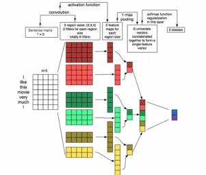
A description OF THE
259
A side OF THE
260
and
261
ONTO THE copy
262
ONTO THE table
263
The similarity between the words picture and copy is calculated as being the average retrieval
264
probability of substituting the word picture with the word copy, i.e., P(<picture, copy>) = (0.5+0.33)/2
265
= 0.415. This is elaborated on the grounds of the combined matching strength between the fragment
266
“A picture OF THE” and the first equivalent class (e.g., 1 / 3 = 0.33 as of having three high frequency
267
words in common with a class having three other members), as well as between the fragment “ONTO
268
THE picture” and the second equivalence class (e.g., 1 / 2 = 0.5 as of having two common high
269
frequency words in common with a class having two other members).
270
271
2.1.1 Distributional semantics
272
273
A long tradition in computational linguistics has shown that contextual information provides a
274
good approximation to word meaning, since semantically similar words tend to have similar
275
contextual distributions [39]. In concrete, distributional semantic models (DSMs) use vectors that
276
keep track of the contexts, e.g., co-occurring words, in which target terms appear in a large corpus as
277
proxies for meaning representations, and apply geometric techniques to these vectors to measure the
278
similarity in meaning of the corresponding words.
279
In this context, vector based approaches take the view that a target word is compared against
280
the vectors for other words in order to determine similarity. For instance, the Pooled Adjacent
281
Context (PAC) model [40] constructs a representation of a word by accumulating frequency counts
282
of the words that appeared in the two positions immediately before and immediately after the target
283
word. The four position vectors created in this way are then concatenated to form the representation
284
of the word. For instance, in the context of the exemplary following windows of text
285
286
found a picture of the found a picture in her a pretty picture of her
found a copy of a found a copy below the destroyed the copy of the
the similarity between picture and copy would have been calculated by setting two vectors with the
287
frequencies of particular words in two positions left and right of the two words in question. For
288
example, the vector of the word copy would be [2 1 0 0 2 1 2 0 1 2 0 1] for all words appearing at
289
positions -1, -2, 1, 2 in all these text windows.
290
Latent Semantic Analysis (LSA)
292
293
LSA [21] takes the idea of extracting lexical meaning of words from the sentential context a little
294
bit further. The underlying idea is that the aggregate of all the word contexts, in which a given word
295
does and does not appear, provides a set of mutual constraints that largely determines the similarity
296
of meaning of words and sets of words to each other. It has been claimed that LSA reflects on human
297
knowledge, which may have been established in a variety of ways. Analytical studies in the past
298
showed that LSA scores overlap those of humans on standard vocabulary and subject matter tests.
299
LSA is also known to mimic human word sorting and category judgments, as well as the way it
300
simulates word–word and passage–word lexical priming data. Finally, it has been reported that it
301
accurately estimates passage coherence, learnability of passages by individual students, and the
302
quality and quantity of knowledge contained in an essay.
303
LSA relies on the follows method. After processing a large sample of machine-readable
304
language, LSA represents the words used in it, and any set of these words, such as a sentence,
305
paragraph, or essay, as points in a very high (e.g. 50-1,500) dimensional “semantic space”. LSA is
306
closely related to neural net models, but is based on singular value decomposition (SVD), a
307
mathematical matrix decomposition technique closely akin to factor analysis that is applicable to text
308
corpora approaching the volume of relevant language experienced by people.
309
More specific, in SVD a rectangular matrix is decomposed into the product of three other
310
matrices. One component matrix describes the original row entities as vectors of derived orthogonal
311
factor values, another describes the original column entities in the same way, and the third is a
312
diagonal matrix containing scaling values such that when the three components are
matrix-313
multiplied, the original matrix is reconstructed. There is a mathematical proof that any matrix can be
314
so decomposed perfectly, using no more factors than the smallest dimension of the original matrix.
315
It is worth noting that similarity estimates derived by LSA are not simple contiguity frequencies,
316
co-occurrence counts, or correlations in usage, as of the previous approaches, but depend on a
317
powerful mathematical analysis that is capable of correctly inferring much deeper relations, e.g., the
318
phrase “Latent Semantic”. As a consequence, these estimates are often much better predictors of
319
human meaning-based judgments and performance than are the surface level contingencies, some of
320
which have been rejected by linguists as the basis of language phenomena.
321
LSA, however, induces its representations of the meaning of words and passages from analysis
322
of text alone. None of its knowledge comes directly from perceptual information about the physical
323
world, from instinct, or from experiential intercourse with bodily functions, feelings and intentions.
324
Thus while LSA’s potential knowledge is surely imperfect, it is believed that it can offer a close
325
enough approximation to people’s knowledge to underwrite theories and tests of theories of
326
cognition.
327
Nonetheless, LSA has some additional limitations. It makes no use of word order, thus of
328
syntactic relations or logic, or of morphology. LSA also differs from some statistical approaches in
329
two significant respects. Firstly, the input data "associations" from which LSA induces
330
representations are between unitary expressions of meaning, i.e., words and complete meaningful
331
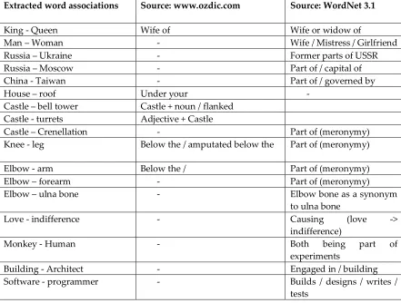
utterances in which they occur rather than between successive words. LSA uses as its initial data
332
not just the summed contiguous pairwise (or tuple-wise) co-occurrences of words but the detailed
333
patterns of occurrences of very many words over very large numbers of local meaning-bearing
334
contexts, such as sentences or paragraphs, treated as unitary wholes. Thus it skips over how the order
335
of words produces the meaning of a sentence to capture only how differences in word choice and
336
differences in passage meanings are related.
337
Another way to think of this is that LSA represents the meaning of a word as a kind of average
338
of the meaning of all the passages in which it appears, and the meaning of a passage as a kind of
339
average of the meaning of all the words it contains.
340
2.1.2 Latent Dirichlet Allocation
344
345
A topic model is a kind of a probabilistic generative model that has been used widely in the field
346
of computer science with a specific focus on text mining and information retrieval in recent years.
347
Since this model was first proposed, it has received a lot of attention and gained widespread interest
348
among researchers in many research fields. The origin of a topic model is latent semantic indexing
349
(LSI) [41]; it has served as the basis for the development of a topic model. Nevertheless, LSI is not a
350
probabilistic model; therefore, it is not an authentic topic model. Based on LSI, probabilistic latent
351
semantic analysis (PLSA) [42] was proposed by Hofmann and is a genuine topic model. Published
352
after PLSA, Latent Dirichlet Allocation (LDA) [22] is treating sentential context in a rather different
353
way than LSA in that it focusses more on associating a document with a topic such as cute animals.
354
Intuitively, given that a document is about a particular topic, one would expect particular words
355
to appear in the document more or less frequently: "dog" and "bone" may appear more often in
356
documents about cure animals. Moreover, a topic model can be represented as a graphical model, or
357
probabilistic graphical model (PGM), or structured probabilistic model. In that sense, a graph
358
expresses the conditional dependence structure between random variables.
359
More formally, LDA is conceived as a three-level hierarchical Bayesian model, in which each
360
item of a collection is modelled as a finite mixture over an underlying set of topics. Each topic is, in
361
turn, modelled as an infinite mixture over an underlying set of topic probabilities. In the context of
362
text modeling, the topic probabilities provide an explicit representation of a document. LDA often
363
relies on efficient approximate inference techniques based on variational methods and an EM
364
algorithm for empirical Bayes parameter estimation [22].
365
In order to exemplify LDA, let us assume that we have the following set of sentences:
366
I like to eat broccoli and bananas.
367
I ate a banana and spinach smoothie for breakfast.
368
Chinchillas and kittens are cute.
369
My sister adopted a kitten yesterday.
370
Look at this cute hamster munching on a piece of broccoli.
371
LDA may have allocated the following probabilities:
372
Sentences 1 and 2: 100% Topic A (food)
373
Sentences 3 and 4: 100% Topic B (cute animals)
374
Sentence 5: 60% Topic A, 40% Topic B
375
Topic A: 30% broccoli, 15% bananas, 10% breakfast, 10% munching
376
Topic B: 20% chinchillas, 20% kittens, 20% cute, 15% hamster
377
In that sense, a document D, which may contain these sentences will be represented with conditional
378
probabilities allocated to topics A and B. In other words, assuming that we have the two food and
379
cute animal topics above, you might choose the document to consist of 1/3 food and 2/3 cute animals.
380
From a machine learning point of view, one has to choose some fixed number of K topics to
381
discover for a given set of documents as you want to use LDA to learn the topic representation of
382
each document and the words associated to each topic. Generally speaking, the algorithm(s) go
383
through each document and randomly assign each word in the document to one of the K topics.
384
Consequently, in order to improve these assignments, for each word w in a document d, and for each
385
topic t, LDA computes two things: 1) p(topic t | document d) = the proportion of words in document
386
d that are currently assigned to topic t, and 2) p(word w | topic t) = the proportion of assignments to
387
topic t over all documents that come from this word w. Subsequently, a new topic is reassigned to w,
388
where the topic t is chosen with probability p(topic t | document d) * p(word w | topic t). Repeating
389
the previous step a large number of times, the algorithm eventually reaches a roughly steady state
390
where the assignments are pretty good.
391
The main disadvantages being reported are associated with the question “how hard it is to know
392
when LDA is working”, since topics are soft clusters so there is no objective metric to say "this is the
393
best choice" of hyperparameters. Metrics like perplexity (how well the model explains the data) can
394
model. For example, you could have a model with very low perplexity, but whose topics are not very
396
informative. Furthermore, LDA and most of its variants rely on a Bag of Words (BoW) approach. In
397
a sense, it still treats documents as a bag of words and the exchangeability of words and documents
398
could be called the basic assumptions of a topic model. These assumptions are available in both PLSA
399
and LDA. Nevertheless, in several variants of topic models, a basic assumption was relaxed.
400
In this context, topic modeling with LDA and its variants does not address the lexical meaning
401
of words as such. It is more seen as a side effect. Moreover, it became obvious that relaxing the basic
402
assumption of LDA or PLSA is a desirable approach, since the availability of many other a priori
403
pieces of information, such as documents’ interactions, the order of words, and knowledge on the
404
biology domain, play an important role as well. In addition, there is significant motivation to reduce
405
the time taken to learn topic models for very large data, for instance, in biological data.
406
2.2. Articifial Neural Networks (ANNs)
407
As already discussed in [44], ANNs are robust learning models that are about precisely assigning
408
weights across many levels. They are broadly divided into two types of ANN architectures: those
409
that can be feed-forward networks and those Recurrent (or Recursive) Neural Networks (RNNs) [45].
410
Feed-forward architecture consists of fully connected network layers. The RNNs model, on the other
411
hand, consist of a fully linked circle of neurons connected for the purpose of back-propagation
412
algorithm implementation. ANNs applied to NLP tasks consider syntax features as part of semantic
413
analysis [46]. New neural network learning models have been proposed that can be applied to
414
different natural language tasks, such as semantic role labelling and Named Entity Recognition [47].
415
The advantage of these approaches is to avoid the need for prior knowledge and task specific
416
engineering interventions. ANN models have achieved an efficient performance in tagging systems
417
with low computational requirements [48].
418
419
Word2vec
420
421
Word2vec [49] can be viewed as a two-layer neural network that processes text. Its input is a text
422
corpus and its output is a set of vectors: feature vectors for words in that corpus. Google calls it “an
423
efficient implementation of the continuous bag-of-words and skip-gram architectures for computing
424
vector representations of words.”
425
While Word2vec is not a deep neural network (see next subsection for more details about deep
426
learning architectures), it turns text into a numerical form that deep networks can understand. In that
427
sense, Word2Vec is a particularly computationally efficient predictive model for learning word
428
embeddings from raw text. For instance, given the sentence “The cat was sitting on the …”, Word2vec
429
is likely to predict the next word being “mat”. Therefore, highly accurate guesses about a word’s
430
meaning can be made, which are based on past appearances. Those guesses can be used to establish
431
a word’s association with other words (e.g. “man” is to “boy” what “woman” is to “girl”), or cluster
432
documents and classify them by topic.
433
The output of the Word2vec neural network is a vocabulary in which each item has a vector
434
attached to it, which can be fed into a deep-learning network or simply queried to detect relationships
435
between words. For instance, a list of words associated with “Sweden” using Word2vec, in order of
436
proximity, is given as of the following vector:
437
The similarity of the word “Sweden” to other words is measured as the cosine similarity between
439
word vectors. Zero similarity is expressed as a 90 degree angle, while total similarity of 1 is a 0 degree
440
angle. For instance, a complete overlap; i.e., Sweden equals Sweden, gives a total similarity of 1, while
441
Norway has a cosine distance of 0.760124 from Sweden, the highest of any other country.
442
The vectors being used to represent words are called neural word embeddings, and representations
443
are strange; one thing describes another, even though those two things are radically different.
444
Word2vec comes in two flavours, the Continuous Bag-of-Words model (CBOW) and the Skip-Gram
445
model. Algorithmically, these models are similar, except that CBOW predicts target words (e.g. 'mat')
446
from source context words ('the cat sits on the'), while the skip-gram does the inverse and predicts
447
source context-words from the target words. This inversion might seem like an arbitrary choice, but
448
statistically it has the effect that CBOW smooths over a lot of the distributional information (by
449
treating an entire context as one observation). For the most part, this turns out to be a useful thing for
450
smaller datasets. However, skip-gram treats each context-target pair as a new observation, and this
451
tends to do better when we have larger datasets.
452
In a nutshell, similar things and ideas are shown to be “close” in that their relative meanings
453
have been translated to measurable distances. Similarity is the basis of many associations that
454
Word2vec can learn. Since words are represented as vectors, powerful mathematical operations can
455
be applied. It was recently shown that the word vectors capture many linguistic regularities, for
456
example vector operations such as vector('Paris') - vector('France') + vector('Italy') results in a vector
457
that is very close to vector('Rome'), and vector('king') - vector('man') + vector('woman') is close to
458
vector('queen'). Despite these information retrieval operations, Word2vec is predominantly a
459
"context predictive" model, which earn their vectors in order to improve the loss of predicting the
460
target words from the context words given the vector representations.
461
462
Global Vectors (GloVe)
463
464
Similar to Word2vec approach, GloVe [50] is another unsupervised learning algorithm for
465
obtaining vector representations for words. The main difference, however, is that training is
466
performed on aggregated global word-word co-occurrence statistics from a corpus, and the resulting
467
representations showcase interesting linear substructures of the word vector space. In that sense,
468
GloVe is usually classified as count-based model, which learn the vectors by essentially doing
469
dimensionality reduction on the co-occurrence counts matrix. Firstly, a large matrix of words x in
470
context y is constructed based on co-occurrence information, i.e., for each "word" (the rows), the
471
learning algorithm counts how frequently we see this word in some "context" (the columns) in a large
472
corpus. The number of "contexts" is, of course, large, since it is essentially combinatorial. Hence,
473
factorization of the matrix is applied in order to yield a lower-dimensional matrix, where each row
474
now yields a vector representation for each word.
475
Deep Learning Architectures
478
479
Deep learning is essentially a bigger take on the neural network models that have been around
480
for some time. It is attribute to Geoffrey Hinton and his first attempts to develop an image
481
classification algorithm. It is, however, particularly useful for analyzing, audio, text, genomic and
482
other multidimensional data that does not lend itself well to traditional machine learning techniques.
483
Word vectors to be used for similarity measures, as previously discussed, can be learned by
484
applying Deep Learning (DL) based architectures as well. DL, as a yet another ANN based
485
architecture, involves multiple data processing layers, which allow the machine to learn from data
486
through various levels of abstraction for a specific task without human interference or previously
487
captured knowledge. Therefore, one could classify DL as unsupervised Machine Learning (ML)
488
approach. Investigating the suitability of DL approaches for NLP tasks has gained much attention
489
from the ML and NLP research communities, as they have achieved good results in solving bottleneck
490
problems [51].
491
These techniques have had great success in different NLP tasks, from low level (character level)
492
to high level (sentence level) analysis, for instance, sentence modelling [52], Semantic Role Labelling
493
[48], Named Entity Recognition [53], Question Answering [54], text categorization [55], opinion
494
expression [56], and Machine Translation [57].
495
More specific, since Deep Learning is based on Convolutional Neural Network (CNN)
496
architectures, which has been around for more than three decades, CNNs have been applied as a
non-497
linear function over a sequence of words, by sliding a window over the sentences. This has been the
498
key advantage of using CNNs architecture for NLP tasks. This function, which is also called a ‘filter’,
499
mutates the input (k-word window) into a d-dimensional vector that consists of the significant
500
characteristic of the words in the window. Then, a pooling operation is applied to integrate the
501
vectors, resulting from the different channels, into a single n-dimensional vector. This is done by
502
considering the maximum value or the average value for each level across the different windows to
503
capture the important features, or at least the positions of these features. For example, Error!
504
Reference source not found. gives an illustration of the CNNs’ structure where each filter executes
505
convolution on the input, in this case a sentence matrix, and then produces feature maps, hence it is
506
showing two possible outputs. This example is used in the sentence classification model.
507
508
A new convolutional latent semantic approach for vector representation learning [58] uses
509
CNNs to deal with ambiguity problems in semantic clustering for short text. However, this model
510
can work appropriately for long text as well [59]. CNNs are proposed for sentiment analysis of short
511
texts that learn features of the text from low levels (characters) to high levels (sentences) to classify
512
sentences in positive or negative prediction analysis. However, this approach can be used for
513
different sentence sizes [60].
514
In a nutshell, building a machine-learning system with features extraction requires specific
515
domain expertise in order to design a classifier model for transforming the raw data into internal
516
representation inputs or vectors. These methods are called representation learning (RL) in which the
517
model automatically feeds in raw data to detect the needed representation. In particular, the ability
518
to precisely represent words, phrases, sentences (statement or question) or paragraphs, and the
519
relational classifications between them, is essential to language understanding.
520
3. Evaluation methodology
521
Evaluating the results of semantic similarity algorithms for the extraction of word associations
522
has proven to be quite complicated. There is mainly due to the following reasons:
523
There is no easy way to define a gold standard, and therefore many different methods
524
of indirect evaluation have been used.
525
The notion of ‘context’ is scattered across a broad spectrum ranging from n-gram
526
models, where context is simply an n-gram, to windowing models, where context is
527
defined as number of words to the left and to the right of the observed word, to a notion
528
of context which means the whole text in which the observed word occurs.
529
The type of the word association being targeted. Roughly speaking, three types of
530
associations may be targeted: syntactic structure, semantic structure, associative structure.
531
The latter is captured in two main flavors:
532
o syntagmatic associations (e.g., run-fast), which are thought to be acquired as
533
consequence of words appearing in succession in the experience of the subject;
534
o paradigmatic associations (e.g., run-walk), which are thought to occur as
535
consequence of experiencing words in similar sentential contexts.
536
Further humbling aspects for easing off the evaluation complexity of these algorithmic approaches
537
have been the variety of algorithms (e.g., type 0, type 1, type 2, type 4), as well as the ways the strength
538
of an association is being measured (e.g., from mutual information, to comparisons of binary and
539
real-valued vectors).
540
Despite the inherited complexity of these evaluation methods, systematic comparisons of
541
algorithms and models have been attempted in the past. For instance, [62] have attempted to
542
quantitatively contrast the abilities of these algorithms to capture all three types of associations,
543
namely, syntactic, semantic and associative information. Much, however, remains to be done to
544
characterize the type of word association each of these algorithms acquire. Moreover, [63] carried out
545
a systematic comparison between context-predicting and context-counting semantic vector
546
approaches, which underpins the differentiation between Word2vec and GloVe semantic vectors.
547
This evaluation, however, does not target all three types of associations and does not give a clear
548
definition of the term ‘word association’.
549
The most promising and most comparable evaluation is one using large manually crafted
550
knowledge sources such as Roget’s Thesaurus [64], WordNet [65-66] or GermaNet for German [67]
551
as a gold standard. Unfortunately, again, evaluations using these sources can be done in many
552
different ways, crippling comparability. A standardized tool set or instance is needed.
553
3.1. Our methodological approach
559
560
After considering the various evaluation methods and the inherited complexity of evaluating
561
the quality of extracted word relations, a conclusion was drawn that for the purposes of this study:
562
the gold standard should probably be
563
either a collocations dictionary like BBI Combinatory Dictionary of English and
564
Explanatory Combinatorial Dictionaries (ECDs),
565
or a semantic net like WordNet.
566
WordNet is a large lexical database of English. Nouns, verbs, adjectives and adverbs are grouped
567
into sets of cognitive synonyms (synsets), each expressing a distinct concept. Synsets are interlinked
568
by means of conceptual-semantic and lexical relations. The resulting network of meaningfully related
569
words and concepts can be navigated with the browser. Apart from gold standards, however, the
570
following pillars expanded our evaluation methodology: psycholinguistic association or priming
571
experiments, vocabulary tests, application-based evaluations, evaluation by using artificial synonyms.
572
Association or priming paradigms [68] can be used to evaluate the results of the algorithms by
573
comparing them with data obtained from human subjects in psycholinguistic experiments. Suitable
574
are association or priming experiments, where subjects are asked to name rapidly some semantically
575
close words after being presented with the stimulus word. The list of most frequently named words
576
can then be compared with the lists obtained automatically.
577
A vocabulary test usually comprises a question and a multiple-choice answer. If both are
578
electronically available, the test can be used quite straightforwardly to evaluate word similarity
579
computation methods. TOEFL, i.e., Test of English as a Foreign Language, has been used as one the
580
tests comprising 80 test items. This kind of evaluation has been used by many authors, such as [69],
581
[21], [70-71].
582
Application-based evaluation is the indirect method of evaluating results of a knowledge
583
extraction algorithm by putting the extracted knowledge into use and observing how well the
584
application using this knowledge performs. One of the most interesting approaches, however, is the
585
use of artificial items. The main idea for testing synonymy is to choose randomly one part of
586
occurrences of a word and replace the word by a pseudo-word while keeping the other part. It is then
587
possible to measure how often the pseudo-words are extracted as synonyms of the words that have
588
been retained.
589
4. Preliminary results and discussion
590
Our comparison study is based on some preliminary results, which have been the outcome of
591
the application of Deep Learning techniques in order to improve the extracted Word2vec model as a
592
means to compute vector representations of words. For the sake of this comparison study, we will
593
refer to the Eclipse Deeplearning4j as an open-source, distributed deep-learning project in Java and
594
Scala spearheaded by the people at Skymind, a San Francisco-based business intelligence and
595
enterprise software firm. Deeplearning4j implements a distributed form of Word2vec for Java and
596
Scala, which works on Spark with GPUs. The extracted word associations, as listed in Table 1, which
597
rely on the trained Word2vec model, have been trained on the Google News vocabulary, which you
598
can import and play with from the Google News Corpus Model
(GoogleNews-vectors-599
negative300.bin.gz, 1,5 GB).
600
For the interpretation of the word associations, the following notations hold: where : means
601
“is to” and :: means “as”. For instance, “Rome is to Italy as Beijing is to China” =
602
Rome:Italy::Beijing:China
603
Table 1: Arrays of extracted word associations
608
1 king:queen::man:[woman, Attempted abduction, teenager, girl]
2 China:Taiwan::Russia:[Ukraine, Moscow, Moldova, Armenia]
3 house:roof::castle:[dome, bell_tower, spire, crenellations, turrets]
4 knee:leg::elbow:[forearm, arm, ulna_bone]
5 New York Times:Sulzberger::Fox:[Murdoch, Chernin, Bancroft, Ailes]
6 love:indifference::fear:[apathy, callousness, timidity, helplessness, inaction]
7 Donald Trump:Republican::Barack Obama:[Democratic, GOP, Democrats, McCain]
8 monkey:human::dinosaur:[fossil, fossilized, Ice_Age_mammals, fossilization]
9 building:architect::software:[programmer, SecurityCenter, WinPcap]
609
Noteworthy is that the Word2vec algorithm has never been taught a single rule of English
610
syntax. It knows nothing about the world, and is unassociated with any rules-based symbolic logic
611
or knowledge graph.
612
Despite the limited number of extracted word associations, these results seem to confirm that
613
the extracted associations do not capture all three types of associations, namely, syntactic, semantic
614
and associative information. and does not give a clear definition of the term ‘word association’. For
615
instance, the word associations King - Queen and Man – Woman do not provide any clue about the
616
type of association holding between these words. There is, however, a semantic structure as a type of
617
association being derived implicitly from the relationship “as” or “same as” holding between the
618
pairs of words {King, Queen} and {Man, Woman}: a King is a Man, a Queen is a Woman. Even so, there
619
is no reference to whether this semantic structure is a hyperonymy, a semantic relation between a more
620
general word and a more specific word, or meronymy, a semantic relation, which refers to a part of a
621
whole and usually characterized as “part-of” relationship.
622
Moreover, there is no such a thing as a pattern of semantic relationships emerging from the first
623
pairs of word associations at both sides of the notation : :. For instance, neither a hyperonymy nor a
624
meronymy seem to be the case for the other word associations on the list, e.g., {monkey, human} and
625
{dinosaur, fossil}, as one cannot infer any relationship between monkey and dinosaur, or between
626
human and fossil. Even if we succeed to identify a pattern of relations, i.e., two large countries and their
627
small, estranged neighbors, such as those emerging from the second row word associations on the list,
628
we cannot emerge victorious with a pattern of semantic relations when we do the same with the
629
eighth row word associations. We will stumble upon questions as to which extent humans should be
630
considered as fossilized monkeys, or humans are what's left over from monkeys, or humans are the species that
631
beat monkeys just as Ice Age mammals beat dinosaurs.
632
An interesting observation has also been as to which extent a holding relationship between two
633
words could imply the same relationship or association type on the other side of the notation : :. For
634
instance, as of the ninth row word associations, and assuming that an architect is-the-designer of a
635
building, can we imply that a programmer is-the-designer of a software? At first glance, it looks like that
636
such a pattern does hold as in most of the cases a well predicted relationship seem to be holding on
637
the other side of the notation : :. There is, however, a notorious difficulty in identifying what are
638
exactly these relations, which can hold on both sides, hence, inferring the one will imply the other.
639
Moreover, [63] carried out a systematic comparison between predicting and
context-640
counting semantic vector approaches, which underpins the differentiation between Word2vec and
641
GloVe semantic vectors.
642
643
4.1 Comparisons with a golden standard (lexicography)
644
645
As indicated in section 3.1, we used as a golden standard the English Collocations Dictionary
646
which is available online at the URL www.ozdic.com, as well as the online version of WordNet 3.1
647
available online at the URL https://wordnet.princeton.edu/ The intention has been to confirm
648
dictionaries, as well as whether the same semantic relationship, be it semantic or lexical, holds across
650
both sides of the notation : : In the following, the results of these comparisons are presented for each
651
list of extracted word associations. All potential relations have been checked bi-directionally, e.g.,
652
entries have been both words King and Queen.
653
Having checked all word entries, we identified two lists, 5 and 7, which have no single
654
collocation. Both lists do predominantly refer to named entities, e.g., Donald Trump, New York Times.
655
Besides, From the total of thirty (30) pairs of associated words, we could identify seventeen (17)
656
collocations in the dictionary, i.e., slightly over 50% of all possible word associations. The following
657
Table 2 summarises the identified collocations together with the potential relations holding between
658
them.
659
660
Table 2: Identified collocations for the English language as of WordNet and ozdic.com
661
Extracted word associations Source: www.ozdic.com Source: WordNet 3.1
King - Queen Wife of Wife or widow of
Man – Woman - Wife / Mistress / Girlfriend
Russia – Ukraine - Former parts of USSR
Russia – Moscow - Part of / capital of
China - Taiwan - Part of / governed by
House – roof Under your
-Castle – bell tower Castle + noun / flanked
Castle - turrets Adjective + Castle
Castle – Crenellation - Part of (meronymy)
Knee - leg Below the / amputated below the Part of (meronymy)
Elbow - arm Below the / Part of (meronymy)
Elbow – forearm - Part of (meronymy)
Elbow – ulna bone - Elbow bone as a synonym
to ulna bone
Love - indifference - Causing (love ->
indifference)
Monkey - Human - Both being part of
experiments
Building - Architect - Engaged in / building
Software - programmer - Builds / designs / writes /
tests
662
Subsequently, we tried to answer the question whether the indicative relations, as indicated by
663
both online resources for the lexical and semantic word meaning, can be projected on the other side
664
of the notation : :. It turned out that almost all of the above relations can be imposed on one or more
665
word associations on either side of the notation : :. For instance, it is perfectly acceptable to impose
666
the relation “wife of” on the word associations {man, woman} and {man, girl}, as well as the relations
667
“amputated below the” or “being part of” for both pairs {knee, leg} and {elbow, arm}. The same holds
668
for the pairs of words {house, roof} and {castle, crenellations}, in terms of the relation “part of”, as
669
well as for the pairs of words {house, roof} and {castle, turrets}, since the expression “roofed house”
670
and “turreted castle” are both meaningful. In some cases, however, e.g., {monkey, human}, the
671
indicative relation cannot be imposed on the other part of the notation : :.
672
Overall, it seems to be indicative that, despite the notorious difficulty to extract the type of
673
association or the relation holding between the pairs of words, some of these word associations do,
674
indeed, make sense according with the lexicographic and semantic meaning of words as indicated by
675
vague and uncertain as the case with sentiments, e.g., in the array fear:[apathy, callousness, timidity,
677
helplessness, inaction].
678
On the other hand, considering the arrays
679
Donald Trump:Republican::Barack Obama:[Democratic, GOP, Democrats, McCain]
680
monkey:human::dinosaur:[fossil, fossilized, Ice_Age_mammals, fossilization]
681
there may be some interesting relations, which remain hidden. For instance, given the fact that
682
Obama and McCain were rivals, it may be interesting to investigate whether the relation “rivalry”
683
may also hold between Donald Trump and the ideal Republican. In addition, the one plausible relation
684
between humans and monkeys may be that humans is the species that beat monkeys just as ice age mammals
685
beat dinosaurs.
686
687
4.2 Comparisons with results from psycholinguistic experiments
688
689
Although it is notoriously difficult to get access to results from psycholinguistic experiments, for
690
the sake of our comparison study, we will mainly refer to results published in [9, 72] and the
Kent-691
Rosanoff Word Association Test in order to study word association norms as a function of age. The
692
experiment has been conducted with 738 subjects from 18 to 87 years of age from various occupations
693
and from various parts of the country. The experiment was meant to study the strength of a word
694
association as a function of age, in terms of a stimulus and response words. For instance, “drinking”
695
as a response to the stimulus word “eating”. Consequently, percentages of subjects responding to 100
696
common word associates for three age groups: Group A: (ages 18-33 years, N= 373), Group B (ages
697
34-49, N = 205) and Group C (ages 50-87, N = 160).
698
Despite the idiosyncratic nature of this experiment and in order to avoid drawing false
699
conclusions, we restricted ourselves in checking for common word entries in the list of 99 words as
700
of [72]. Our comparisons verified that it is difficult to infer any semantic or lexical relations holding
701
among the associated words. Hence, from this comparison, there is no directly added value in
702
predicting what the potential relation may be, or whether the “same as” predicate on both sides of
703
the notation : : can be added.
704
It has been revealed, however, that few of the word associations in our nine (9) arrays of Table 1
705
do also exist in the results of this experiment. For instance, the associations between man and woman,
706
kind and queen, could also be confirmed. The most revealing aspect, however, has been that
707
associations within the same array of associated words, such as between woman and girl could be
708
unveiled by the entries in the list of 99 words [72]. This may, in turn, indicate, the associations may
709
be transitive as well. For instance, the association between man and girl may be the result of the
710
associations between man and woman, as well as woman and girl.
711
4. General discussion
712
In this paper, we discuss some preliminary results and emerging trends and how they can be
713
interpreted in perspective of previous studies, including our own comparisons. The main working
714
hypothesis has been the question(s) as to what are the limitations of Deep Learning (DL), not only for
715
the extraction of word meaning in natural language processing, but also for the extraction of
716
meaningful associations among objects or entities, in general.
717
The experimental design addressed primarily a DL framework for the following main reasons:
718
a) to demystify the prowess of this ANN based architecture in its capacity to computationally
719
recognize and understand in terms of interpreting associations between words, b) to act as a typical,
720
up to date, representative of machine learning algorithms for natural language processing and
721
understanding, c) to unveil future research directions, d) to establish an evaluation framework for
722
future reference.
723
Therefore, it is this broader context within which our findings and comparison results should be
724
interpreted, although rather limited than with some statistical significance. Nevertheless, the