The Limpet: A ROS-Enabled Multi-Sensing Platform for the ORCA
Hub
Mohammed E. Sayed1, Markus P. Nemitz1,2*, Simona Aracri1*, Alistair McConnell1, Ross M. McKenzie1,3, and Adam A. Stokes1**
SUPPLEMENTAL INFORMATION
1School of Engineering, Institute for Integrated Micro and Nano Systems, The University of Edinburgh, Scottish Microelectronics Centre, Alexander Crum Brown Road, King's Buildings, Edinburgh, UK , EH9 3FF
2Department of Computer Science and Engineering, University of Michigan, 2260 Hayward St. BBB3737, Ann Arbor, MI, 48109 USA
3Engineering and Physical Sciences Research Council (EPSRC) Centre for Doctoral Training (CDT) in Robotics and Autonomous Systems, School of Informatics, The University of Edinburgh, Edinburgh EH9 3LJ, UK
* These authors contributed equally to this work.
Supplemental Figures
Figure S3: A picture of the 3D printed mold used to design the protective housing of the Limpet.
converter, which converts this data into a ROS protocol. The data can be published to a ROS topic and based on the label sent with the data, the converter can decide which topic to publish the data to. Any ROS node can subscribe to a specific ROS topic to read the sensor data.
Figure S6: Overview of the communication strategies. The communication bandwidth decreases and the on-board computational power increases as we move from WiFi to optical
communication. A) Overview of components involved in WiFi communication. In this
communication strategy, the sensor data is fed into the microcontroller, which is then sent in real time to the PC. Transmission of data over WiFi is achieved using the ESP8266, a SOC WiFi module with integrated TCP/IP protocol stack that gives the Limpet access to the WiFi network. The data can then be analysed on the PC. B) Overview of components involved in serial
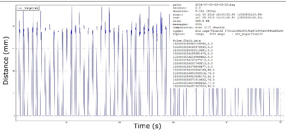
Figure S8: A plot of the power density data versus time from the optical sensor when transmitting numbers using the red LED. Each consecutive peak corresponds to a number from 9 to 0.
Figure S10: A plot of the power density data versus time from the optical sensor when
transmitting numbers using the blue LED. Each consecutive peak corresponds to a number from 9 to 0.
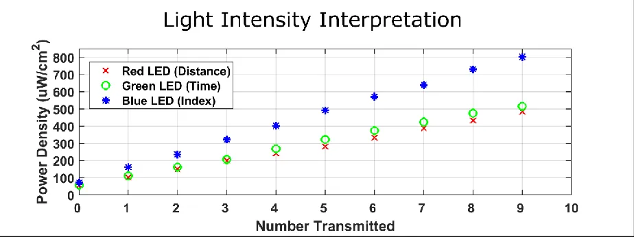
Figure S11: Light intensity interpretation for optical communication. This graph shows how the power density of the RGB LED represents a number transmitted by the Limpet. The red LED is used to send information about distance, green LED is used for timestamp information and blue LED is used for index information. The different power density for each LED corresponds to a number on a scale of 0 to 9. The different power densities are achieved by pulse-width
Figure S15: Down-sampling results from WiFi communication.This figure shows the effect of down-sampling on the sensor data, which was transmitted via WiFi, after removing the outliers and applying the low-pass filter. The sensor data was recorded over a period of 300 seconds. Our down-sampling method decreases a signal’s length to a number of averaged data points
for fault 1 operation mode. C) This graph shows down-sampled data for fault 2 operation mode. D) This graph shows sampled data for fault 3 operation mode. E) This graph down-sampled data for fault 4 operation mode.
Figure S16: A figure showing the raw sensor data transmitted by the Limpet via serial
Figure S25: Results of the experiments using LoRa and optical communication. The LoRa and optical communication experiments were conducted separately. This figure shows the down-sampled results from LoRa communication and optical communication when we introduce the four faults to the system, and the spectral analysis done on the down-sampled results for each of the faults. The down-sampled results are shown within a period (T) of 3.2 seconds
(corresponding to the frequency of rotation of the fan during normal operation. The figure also shows the colour power density from the optical sensor during the transmission of data. The graph contains information on the distance, timestamp and index of the measurement. The red peaks represent distance data, green peaks represent time data, and blue peaks represent index data. For each measurement, 2 distance data points are transmitted (2 red peaks), 4 timestamp data points are transmitted (4 green peaks), and 3 index data points are transmitted (3 blue peaks). A) Schematic of the first fault introduced to the system. B) This graph shows the colour power density from the optical sensor when fault 1 is introduced to the system. C) This graph shows the down-sampled result from the distance measurement, which is transmitted via LoRaWAN network and optical communication, after introducing fault 1 to the system. The optical communication results are constructed from the optical sensor data. Every two
smaller peaks around frequencies of 0.35 Hz, 0.7 Hz and 1 Hz. The peaks at 1.3 Hz represents the fan blade with the attached object, while the other peaks represent the other three fan blades. E) Schematic of the second fault introduced to the system. F) This graph shows the colour power density from the optical sensor when fault 1 is introduced to the system. G) This graph shows the down-sampled result from the distance measurement, which is transmitted via LoRaWAN
representing the normal fan operation and another peak at a lower frequency representing the fault introduced to the system.
data after elimination of outliers. C) Sensor data after application of low-pass filter. D) Down-sampled sensor data. E) Distance profile. F) Power spectral density.
frequency is lower than Nyquist frequency, showing that normal or fault measurands can not be identified. The sensor data was transmitted via WiFi. A) Raw sensor data. B) Sensor data after elimination of outliers. C) Sensor data after application of low-pass filter. D) Down-sampled sensor data. E) Distance profile. F) Power spectral density.
Figure S29: A figure showing an experiment conducted with a sampling rate lower than frequency of blade rotation. The sampling frequency used in this experiment is 1Hz. The frequency is lower than Nyquist frequency, showing that normal or fault measurands can not be identified. The sensor data was transmitted via serial communication. A) Raw sensor data. B) Sensor data after elimination of outliers. C) Sensor data after application of low-pass filter. D) Down-sampled sensor data. E) Distance profile. F) Power spectral density.