Data Transmission Plan Adaptation Complementing
Strategic Time-Network Selection for Connected Vehicles
Tobias Rueckelto∗, Ioannis Stavrakakis+, Tobias Meuser∗, Imane Horiya Brahmi#, Doreen B¨ohnstedt∗, Ralf Steinmetz∗
∗Multimedia Communications Lab (KOM), Technische Universit¨at Darmstadt, Germany
+National and Kapodistrian University of Athens, Greece – IMDEA Networks & UC3M, Spain #University College Cork & Tyndall National Institute, Cork, Ireland
oDaimler AG, Stuttgart, Germany
Abstract
Connected vehicles can nowadays be equipped with multiple network interfaces to access the Internet via a number of networks. To achieve an efficient transmis-sion within this environment, a strategic time-network selection for connected vehicles has been developed, which plans ahead delay-tolerant transmissions. Under perfect prediction (knowledge) of the environment, the proposed strategic time-network selec-tion approach is shown to outperform significantly leading state-of-the-art approaches which are based either on time selection or network selection only. Under realistic environments, however, the efficiency of planning-based approaches may be severely compromised since network presence and available capacities change rapidly and in an unforeseen manner (because of changing conditions due to the uncertainty in car move-ment, data transmission needs and network characteristics). To address this problem, a mechanism is proposed in this paper that determines the deviation from the antic-ipated conditions and modifies the transmission plan accordingly. Simulation results show that the proposed adaptation mechanisms help maintain the benefits of a strategic time-network selection planning under changing conditions.
1. Introduction
Nowadays, mobile nodes typically integrate different wireless network interfaces. An example environment of wireless networks is shown in Figure 1, covering one mo-bile network (yellow) and three WiFi networks (blue, green, red) that are available for limited time spans during the trip. To improve connectivity performance, connected
5
vehicles may use these networks in parallel to distribute their data traffic. Moreover, the connected vehicle use case provides an additional optimization potential, especially considering automated vehicles: Routes are usually known and, thus, movement can be predicted accurately. As a result, a vehicle can predict future network availability and characteristics using the so-called connectivity maps [1, 2]. A derived prediction
10
of network availability over time is visualized in Figure 1 using colored bars. Further-more, according to Sandvine [3], a major part of a mobile node’s data traffic is delay-tolerant or heavy-tailed. Assuming networks and data traffic to be roughly known for a certain time horizon, we show in prior work [4] that a transmission planning can provide significant benefits. The transmission planning approach combines network
15
selection [5] with a selection of the transmission time [6]. The approach plans ahead data transmission over multiple networks. In this paper, we present additional insights on the performance characteristics of this approach. However, the presented approach assumes perfect prediction of vehicle movement, network characteristics and data to transmit, as visualized in Figure 2 left. Such accurate prediction might not always be
20
available. In the real world, further mechanisms have to cope with prediction errors. Accordingly, we present three contributions in this paper:
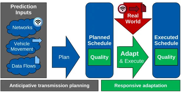
1. A strategic time-network selection approach that maximizes transmission effi-ciency using heterogeneous wireless networks due to transmission planning (Fig-ure 2 blue arrow).
25
2. An investigation of the effects of erroneous prediction on the performance of transmission plan execution (Figure 2 red arrow)
Mobile Network
WiFi 1
WiFi 2
WiFi 3
[Time]
[Ne
tw
or
k]
Figure 1: Connected vehicle using heterogeneous wireless networks: example scenario
Prediction Inputs
Networks
Vehicle Movement
Data Flows
Plan
Planned Schedule
Quality Execute
Executed Schedule
Quality
Execute QualityQuality
Adapt
& Execute
Real World
Anticipative transmission planning Responsive adaptation
Figure 2: System overview: prediction-based transmission planning complemented by adaptation for plan
In Section 2, we briefly outline our previous work on an anticipative data
transmis-30
sion planning assuming static conditions and perfect knowledge of the environment and compare it to an Opportunistic Network Selection (ONS) (no planning or predic-tion). We show its performance characteristics in different scenarios and compare it also to other state-of-the-art-based approaches. Furthermore, we introduce our predic-tion error models and show that the performance of the strategic time-network selecpredic-tion
35
approach degrades severely in the presence of prediction errors, due to its inability to react to changing conditions. In contrast, the opportunistic approach – although un-derperforming with respect to the transmission plan approach under static conditions and perfect knowledge – appears to deliver a constant performance in the presence of prediction errors. This provides the motivation for our proposed transmission plan
40
adaptation mechanism, presented in Section 3, which complements the transmission planning. The benefit of each planned transmission is re-evaluated and the planned transmission is modified by invoking a constrained ONS taking into account the type and magnitude of condition changes (i.e., car movement, data flows or network char-acteristics); mechanisms detecting relevant condition changes are also introduced. In
45
Section 4, we discuss the performance of our novel adaptation approach under various changing conditions, followed by a related work discussion in Section 5. It turns out that our responsive adaptation approach can largely sustain the gain foreseen from an-ticipative transmission planning with strategic time-network selection under small to moderate changes in the environment.
50
2. Data Transmission Planning
The predictable movement of multi-homed mobile clients enables a transmission planning over networks and time. In our prior work [4], we demonstrate significant benefits of such a planning in comparison to state-of-the-art approaches. In this section, we summarize the approach, the evaluation metrics and results of this work and extend
55
2.1. Evaluation Metrics and Model of Forces
To assess the efficiency of our strategic time-network selection approaches, we developed a performance rating function, that captures application QoS requirement
60
satisfaction and monetary cost. We bisect the performance rating function into two components that are in effect in a mutually exclusive manner depending on whether data is allocated or not. We call the first component the attracting forcescattr. It cap-tures cost associated with data that is not allocated to a network, punishing the violation of a minimum throughput requirement and the amount on non-allocated data. The
sec-65
ond component, referring to as the repelling forcescrep, captures cost associated with data that is allocated to a network, punishing the violation of the QoS requirements of the data flows or monetary transmission cost. It covers components from network selection, like latency, jitter and also components from transmission time selection approaches, including deadline and the preferred start time of data transmissions, as
70
visualized in Figure 3.
Networks attract data for allocation in general throughcattr, creating attracting forces for each data flow according to its priority. In addition, the repelling forces push data away from networks and time slots that cannot satisfy the data flow’s QoS requirements. The rating function in Equation (1) adds the two mutually exclusive
75
components for a given transmission planp. Note thatp∗is an alias forp, indicating that the given model component punishes the absence of a desired transmission in a plan.
c(p) =cattr(p∗) +crep(p) (1)
Minimizing the cost function results in a data allocation to the best matching
net-80
works at matching points in time over the complete planning time horizon. For the detailed model of the cost function, refer to [4]. It is summarized in Figure 3.
As the absolute value of the cost in Equation (1) strongly depends on the scenario, a Normalized Rating Score (NRS) is introduced to allow for a meaningful comparison of multiple scenarios.NRS describes a transmission plan’s achieved share of the absolute
Attracting forces Non-allocated data
throughput requirement violation
Data isnotallocated
Foster transmission
Repelling forces
Latency and jitter violation
Monetary cost
Start time and deadline violation
Data isallocatedwith violations
Suppress transmission with violations
Figure 3: Transmission rating using a model of forces
optimization potential of the given scenario.A value of 0.8 means that a transmission plan uses 80% of the scenario’s optimization potential. To define the optimization potential, we employ an upper and a lower cost bound. As a lower cost bound, we use the cost of an optimal transmission plan. As an upper cost bound, we use the average cost of random transmission plans. We assume this as a reasonable upper cost bound
90
for rating because no transmission plan, which was created with intent, should perform worse than random. Higher values are still feasible.
2.2. Transmission Planners
Transmission planners determine data allocation to networks and over time. We analyze three transmission planners from [4] in this paper and an additional one for
95
transmission time selection. All of them use the same ratings for network selection and data flow prioritization to create comparability of their results. However, they differ in the way they handle the time dimension.
The first is aNetwork Selection (NS)is derived from state-of-the-art approaches and allocates data to thecurrentlyavailable networks ignoring the time dimension. It
100
prioritizes data flows and decides for each one, whichcurrentlyavailable networks are best suited for its transmission. Finally, it allocates data according to these priorities. Note that it transmits in a best effort fashion, utilizing the selected networks at their maximum transmission rate.
As a second approach, we present anOpportunistic Network Selection (ONS). It extends Network Selection by considering an opportunistic component, which decides whether to transmit data(as the NS would dictate)or not. This decision is based on an estimated benefit, defined as the difference between the estimated repellingc
(in case data is transmitted) and the estimated attractingc
g attr(p
∗
f,t,n)(in case data is not transmitted) forces. Whenever the benefit exceeds some thresholdclim, the approach allocates data to the network. This is shown in Equation (2), showing the cost differ-ence for a specific data allocation of data flowf at time slottto networkn. Rejecting non-beneficial transmission at the current point in time amounts to waiting for a better opportunity to transmit.
c
g attr(p
∗
f,t,n)−cgrep(pf,t,n)> clim (2)
In addition to these two network selection approaches, we presentDelayed WiFi
105
Offloading (DWO)as a leading approach from the transmission time selection domain. It ignores the flow-network matching and follows a basic WiFi-preferred strategy, not considering most QoS requirements of data flows. The approach seeks to transmit as much data as possible via WiFi. Therefore, it plans ahead data transmissions of delay-tolerant data flows, assigning their transmission to a point in time when WiFi networks
110
are assumed to be available. Hence, it requires a prediction of network availability and data rates. The transmission delay is determined by considering a maximumplanning time horizoncomplying with the prediction time period and the data flow’s deadline. These three approaches are generalized from leading state-of-the-art approaches and serve for performance comparison to our own approach, presented in the following.
115
As a fourth approach, we present ourJoint Transmission Planning (JTP), as in-troduced in [4]. Instead of considering the currently available networks only, JTP se-lects thebest transmission opportunities within the complete planning time horizon. Thus, it combines the planning concept from transmission time selection with an elab-orated flow-network matching from network selection. It plans data allocation ahead
120
for a time, in which the transmission is expected to be most beneficial. In addition, it uses the opportunistic component from ONS to be able to move delay-tolerant trans-missions beyond the planning time horizon in case of insufficient transmission oppor-tunities. Hence, it represents a strategic time-network selection, which handles both dimensions, time and networks, explicitly. However, the approach requires a
predic-125
0.4 0.6 0.8 1
Networks
Normalized
Rating
Score
(NRS)
DWO NS ONS JTP
1 2 4 8 16 32
0.4 0.6 0.8 1
Networks
Normalized
Rating
Score
(NRS)
0.4 0.6 0.8 1
Data traffic Load
Normalized
Rating
Score
(NRS)
DWO NS ONS JTP
low medium high
0.4 0.6 0.8 1
Data traffic Load
Normalized
Rating
Score
(NRS)
Figure 4: Normalized Rating Score (NRS) of the transmission planners for different number of networks in
the planning time horizon (left) and different amounts of data traffic of the vehicle (right)
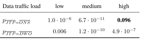
Table 1: T-test results over number of networks forH0: J T P=ON SandJ T P=DW O
Networks 1 2 4 8 16 32
pJ T P=ON S 0.81 0.47 3.7·10−6 1.8·10−7 2.8·10−10 1.9·10−7
pJ T P=DW O 0.74 0.43 0.14 3.2·10−7 2.6·10−8 3.5·10−9
Table 2: T-test results over data traffic load forH0: J T P =ON SandJ T P =DW O
Data traffic load low medium high
pJ T P=ON S 1.0·10−6 6.7·10−11 0.096
We simulate the different approaches with default parameters of a planning time horizon length of 100 time slots (1 second each), 8 networks (2 mobile, 6 WiFi) in the planning time horizon, a medium amount of data traffic that utilizes about 70% of
130
the available network resources, consisting of 8 individual data flows. Characteristics follow a default mobile data traffic distribution [3]. Figure 4 presents the Normal-ized Rating Score results of the transmission planners for different number of networks (1 to 32) in the planning time horizon and for different amounts of data traffic (low, medium, high) of the vehicle. More details about the simulation setup are available
135
with the source code for reproducibility and possible extension of this work, see ac-knowledgments.
Under varying number of networks, the Network Selection (NS, as a dashed light blue line) and Opportunistic Network Selection (ONS, as a dotted magenta line) show similar trends. They perform well with a median NRS of 79-86% when there is just a
140
single or two networks available within the planning time horizon. However, in these scenarios, there is not much choice which makes selection almost obsolete. Accord-ingly, all approaches perform well. As soon, as there are several networks to select from, i.e. there exists a certain optimization potential in the scenario, their perfor-mance drops significantly to median 67%, respectively 74%. For a large number of
145
networks, their relative performance starts to recover. The reason for that is a satu-ration of ”good” networks in the scenario, meaning that for a large number of net-works within the planning time horizon, there is a good network available at nearly any point in time, rendering time selection obsolete. The two effects lead to an inverse performance characteristic for the transmission time selection approach Delayed WiFi
150
Offloading (DWO, dash-dotted dark blue).
These results show that our strategic time-network selection approach Joint Trans-mission Planning (JTP, green solid) yields always high performance of 87-91% of the optimization potential. JTP outperforms the state-of-the-art approaches in average by 15.47% (NS), 7.71% (ONS) and 7.26% (DWO). Table 1 presents the t-test results of
155
bold. The results dignify that that the observed performance gains of our approach JTP are significant as soon as the scenario covers a couple of networks, i.e. there exists a
160
certain optimization potential in the scenario.
Figure 4 right shows the evaluation results for scenarios in which the vehicle trans-mits a different amount of data. With a rising amount of data traffic NS and ONS per-form better. Again, this is linked to the optimization potential of the scenario. When a lot of data has to be transmitted, nearly every transmission opportunity has to be used.
165
Hence, there is little flexibility in leaving out unfavorable transmission opportunities which renders transmission time selection less important. Accordingly, network se-lection approaches perform relatively better under high data load. In contrast, DWO which lacks an appropriate network selection shows an inverse characteristic. It per-forms better in scenarios with low data traffic providing a high flexibility for leaving
170
out transmission opportunities.
Our strategic time-network selection approach JTP, which combines the advantages of the three approaches generalized from state-of-the-art, shows superior performance for all scenario variations, reaching again 87-91% of the optimization potential. JTP outperforms the state-of-the-art approaches in average by 18.23% (NS), 8.41% (ONS)
175
and 10.90% (DWO). As shown from the t-test results in Table 2, if there is a certain optimization potential, these performance gains are significant.
Conclusively, the results demonstrate the huge benefits of a strategic time-network selection. It achieves a significantly higher transmission efficiency of up to 18% when using heterogeneous wireless networks.
180
The results for the strategic time-network selection approach JTP in Figure 4 are derived assuming perfect knowledge of the environment, i.e. network resources and demand characteristics. As this can hardly be the case in real environments, predictions about the state of the environment in the future will not be perfect, as indicated in Figure 2 with the red arrow. In the remainder of this paper, we first introduce prediction error
185
3. Adaptation of Transmission Plans
Transmission plans are applicable whenever prediction is correct. Nevertheless,
190
what does happen if the prediction used for transmission plan creation is erroneous? In this section, we analyze prediction error types of the connected vehicle use case and design a novel adaptation approach with the goal of robustness against this kind of uncertainty.
3.1. Prediction Errors
195
In a connected vehicle environment, as exemplified in Figure 1, transmission plans can be derived based on some predictions on the vehicle movement, the encountered network characteristics and the data to be transmitted. As such predictions may be incorrect, it is important that resulting prediction errors are calculated and some adjust-ments in the transmission plan are made. The Symmetrical Mean Absolute Percentage
200
Error (SMAPE) [7] is employed to measure those prediction errors. The movement prediction error mainly affects the availability of networks. For example, a vehicle, which moves faster than expected, may reach a small range network earlier and may spend less time in its covered area. We measure the error in the number of time slot drifts over the planning horizon. The network characteristics prediction error affects
205
the throughput, latency and jitter of the networks over time. Finally, the data flow prediction error arises from canceling or pausing running data transmissions or from unexpected new data transmissions. Next, we present our adaptation approach handling these three types of errors.
3.2. Adaptation Approach
210
The idea of our adaptation approach is to use a constrained Opportunistic Network Selection (ONS) whose decision thresholdclimis determined according to environ-mental changes so that the data transmission plan that is actually implemented is still beneficial. First, we design a transmission plan execution algorithm, which constraints ONS to implement the initial transmission plan, when no environmental changes
oc-215
present three adaptation mechanisms that dynamically relax the constraints and modify parameters of the first algorithm.
Execution Algorithm (Exec): To follow an initial transmission plan, this algorithm suppresses each data transmission, which does not comply with the plan. Therefore,
220
the mechanism increases the benefit thresholdclim of the base approach ONS to the flow’s maximum benefit valuecmax(f, t), defined as the supremum of its attracting force according to Equation (3). When, in contrast, data is allocated in the initial plan, it sets the threshold to the flow’s minimum benefit valuecmin(f, t), defined as the infimum of its repelling forces, which is based on the highest requirement violations
225
from the currently available networksN0according to Equation (4). To decide which
of the two threshold values to use, the approach compares the amount of released data prel(f, t
0)from Equation (5) to the actually allocated datasalloc(f, t0)of data flow f from Equation (6) at the current time slott0according to Equation (7). While the
released dataprel(f, t
0, n)does not change over time within the considered time slot,
230
the value of the allocated datasallocis refreshed continuously, stopping the allocation as soon as the amount of the data planned for the current time slot is transmitted. This completes the ONS-based transmission plan execution algorithm. In the following, we enhance this algorithm with mechanisms for transmission plan adaptation as a reaction to recognized prediction errors of the networks, the node movement and the data flows.
235
cmax(f, t) = sup t∈T
cattr(p∗f,t,n) (3)
cmin(f, t) = inf n∈N0
crep(pf,t,n) (4)
prel(f, t0, n) =pf,t0,n (5)
clim=
cmin(f), salloc(f, t0, n)< prel(f, t0, n)
cmax(f), else
(7)
3.2.1. Extended Data Release Mechanism
Our first adaptation mechanism addresseschanges in the network characteris-tics. This corresponds, firstly, to changed transmission characteristics like latency and jitter and, secondly a differing throughput. Changes in network characteristics may affect the flow-network matching and preference. Strong performance degradation of
240
networks might lead to the case in which transmission is not beneficial at all. To let the constrained ONS decide whether to transmit or not, we set the minimum thresh-oldcmin to the ONS’s default value 0 according to Equation (8). Other values would be feasible as well. Higher values restrict transmission to opportunities with a higher benefit. This may lead to a better flow-network matching but may also suppress some
245
transmissions completely. The value0provides a good trade-off. It restricts each data allocation to the cases for which ONS still considers a sufficient benefit. In addition, we relax constraints to employ ONS for re-evaluation of the flow-network matching and a re-selection using the actual network characteristics. Therefore, we stop distin-guishing between networks for releasing data. To this end, we constrain all networks in
250
the current time slot equally by considering the sum of allocated data over all networks, as shown in Equations (9) and (10).
To address unbiased fluctuations of the network throughput, we relax the execution algorithm’s limit for the amount of released data. Instead of focusing on the amount of data planned for transmission for each time slot separately, we redefine the released
255
dataprel(f) according to Equation (9) to cover all data allocated in the initial plan until the current point in timet0 plus the flow’s data, which has not been allocated
in the initial plan at allp∗f. Thus, data may also be allocated at good transmission opportunities after the planned transmission time. This helps the approach to cope with unbiased fluctuating network throughput and allows the constrained ONS to fill
260
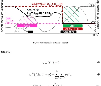
time
ONS: clim=0
Ada(JTP):
clim= cmax(f) * α(f,t0)
Ada(JTP) be ne fit for toke n al lo catio n ONS JTP Ada(JTP)-rel Ada(JTP)-rel: clim= cmax(f)
amo un t of rel ea sed da ta 0% 100% allocated data
Figure 5: Schematic of basic concept
datap∗f.
cmin(f, t) = 0 (8)
prel(f, t0, n) =p∗f+ t0
X
t=0
X
n∈N
pf,t,n (9)
salloc(f, t0, n) =
t0
X
t=0
X
n∈N
sf,t,n (10)
Figure 5 visualizes the characteristic behavior. Firstly, it shows the benefit over time for allocating data as a black thin curve. Allocating data with higher benefit leads to a lower cost function value, representing a better transmission. In addition, the figure
265
contains lines for the cost benefit thresholdclimof ONS (pink). ONS setsclim= 0by default, thus allocating data at the earliest point in time offering a transmission benefit. In the example, ONS transmits during the first benefit ’hill’, during the pink marked time span. We consider the transmission to be finished after that time span in the example. In contrast, the Joint Transmission Planning approach (JTP, green) allocates
270
data at the transmission opportunity with the highest benefit; in the example the second ’hill’.
suppresses data transmission until the plan of JTP holds allocations. Thus, a data
allo-275
cation in the plan allows the mechanism to transmit data opportunistically. In case of no prediction errors, this results in setting the cost benefit thresholdclimaccording to the red line, which lets this adaptation mechanismAda(JTP)-relstay close to the initial plan.
3.2.2. Location reference mechanism
280
To cope withmovement prediction errors, we present our corresponding adap-tation mechanism, which refers to the initial plan by vehicle location instead of time. When a vehicle moves e.g. faster than predicted, it reaches and leaves short range networks earlier than expected. Compared to the prediction, location dependent net-work characteristics move to another point in time. As a result, netnet-work availability is modified from the initial time-line, impairing on the network selection of the trans-mission plan. Furthermore, for delay-tolerant data transfers, it is more important to sustain the network-matching then to sustain the selected transmission time. To ad-dress this issue, we employ the following mechanism: For delay-tolerant data flows, consider the spatial dimension in the transmission plan, i.e. the vehicle’s location, and ignore the temporal one. Referring to the spatial dimension is equivalent to a tempo-ral offsetmove(t0)of the transmission plan. The location reference mechanism shifts
data transmission in time by this temporal offset to preserve the initial network selec-tion. However, for non-delay-tolerant data flows, e.g. interactive ones, this temporal transmission offset may lead to a temporal requirement violation. Hence, we limit the temporal offsetmove(t0)to the maximum delay-tolerance of the data flow, which our
model from prior work [4] encodes in a throughput requirement window parameter ∆btminf , c.f. Equation (11). Accordingly, we employ the time-limited spatial reference tloc(f, t0)according to Equation (12) to refer to the initial plan. This limited spatial
reference preserves the initial network selection of the transmission plan for delay-tolerant data flows but accounts temporal requirements for non-delay-delay-tolerant flows.
tof f setf = min(∆bt min
tloc(f, t0) =
t0+tof f setf , move(t0)>0
t0−tof f setf , else
(12)
Referring to the corresponding vehicle location in the transmission plan to release data for allocation in the presented manner causes one problem: whenever the car stops, no additional data is released. There is no progress in the vehicle’s location and, thus, the transmission pauses. This effect impairs transmission similarly when the car moves slower than expected. To address this issue, our mechanism modifies the
285
condition for theclimthreshold selection of Equation (7) to that from Equation (13). Whenever data is allocated within the initial plan in the reference time slot, release data for transmission.Hence, this mechanism together with the extension in triggering conditions handles movement prediction errors up to a certain degree.
salloc(f, t0, n)< prel(f, tloc(f, t0), n)
or X
n∈N
pf,tloc(f,t0),n
! >0
(13)
3.2.3. Flow Prediction Error Handling
290
to0, we reduce cmax with rising error according to Equation (14) and (15). Thus, when flow prediction errors occur, our approach does not suppress data allocation but restrict it to opportunities in which an error-dependent benefit threshold is reached. We illustrate an example threshold adaptationα(f, t0)from Equation (14) in Figure 5
with a thick black line. In the example, this results in a partially earlier transmission of Ada(JTP). The final transmission plan adaptation mechanism is given in Equation (16).
α(f, t0) = 1−
t0
X
t=t0−∆btminf
f low(f, t)
∆btminf
(14)
cmax(f, t0) = sup
t∈T
cattr(p∗f,t,n)·α(f, t0) (15)
Final adaptation algorithm threshold:
clim=
0,
salloc(f, t0, n)< prel(f, tloc(f, t0), n)
or X
n∈N
pf,tloc(f,t0),n !
>0
supt∈Tcattr(p∗f,t,n)·α(f, t0), else
(16) Conclusively, our transmission plan adaptation approach combines the advantages of Opportunistic Network Selection and Joint Transmission Planning. Thus, it allows for opportunistic transmission when high prediction errors render parts of an initial plan infeasible but can exploit the superior transmission patterns in terms of time and network selection from anticipative transmission planning. We evaluate the effects
295
of the execution (Exec) and the three adaptation mechanisms (Ada) within the next section.
4. Evaluation
To analyze the performance of the transmission plan adaptation mechanism (Ada), we assess its performance under controlled variation of the prediction errors with the
300
performance reference, we show the results of Joint Transmission Planning (JTP) with perfect prediction. JTP uses this perfect prediction for all modified scenarios, inde-pendent from the defined error on the x-axis. It defines an upper bound for reference.
305
We apply the different approaches to scenarios with 100 time slots, covering 2 cellular networks and 6 WiFi networks, which are available within the scenario’s planning time horizon. The number of data flows is initially 8 and varies due to flow prediction errors. We apply the different approaches to 50 randomized scenarios per run. For execution of each instance, we use a single core of a server machine with Intel Xeon E5-2643 v3
310
@ 3.4GHz and 512 GB RAM. To show the typical performance and its distribution, we give theQ25%,Q50%(median) andQ75%quantiles. We vary the prediction errors
(SMAPE) separately for movement, network characteristics, data traffic and finally for a combined one between 0.0 and 0.5. We let the adaptation approach follow the plan of JTP and abbreviate the different mechanisms with (1) Ada(JTP)-rel: ONS with the
315
data release mechanism (2) Ada(JTP)-rel-loc: with additional location reference mech-anism and (3) Ada(JTP): the final approach covering all three mechmech-anisms.
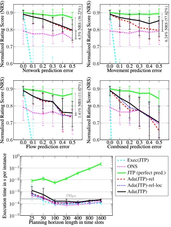
The results are presented in Figure 6, showing the graphs for each of the error types and the combined case. First of all, we notice that in presence of environmental changes the pure execution of the plan Exec(JTP) (dashed light blue) suffers substantially from
320
robustness. It sinks far below the performance of ONS even for small prediction errors. This performance drop demonstrates that a pure execution is not efficient in reality and an adaptation is required.
In contrast, the performance of our adaptation approach (black solid) stays approx-imately between those of JTP and ONS, starting at the JTP’s and converging towards
325
the ONS’s performance for rising errors. Increasing the network prediction error (a) shows that our basic data release mechanism Ada(JTP)-rel (dashed red) is able to han-dle this error type well. Even at an error of 0.5, the adaptation sustains a gain from anticipative transmission planning of about 4.5% NRS over ONS which corresponds to 36.23% of the performance margin between JTP and ONS. However, the basic data
330
is-0.0 0.1 0.2 0.3 0.4 0.5 0.6
0.7 0.8 0.9
4.5%
NRS
(36.23%)
Network prediction error
Normalized
Rating
Score
(NRS)
0.0 0.1 0.2 0.3 0.4 0.5 0.6
0.7 0.8 0.9
Network prediction error
Normalized
Rating
Score
(NRS)
0.0 0.1 0.2 0.3 0.4 0.5 0.6
0.7 0.8 0.9
6.24%
NRS
(57.62%)
Movement prediction error
Normalized
Rating
Score
(NRS)
0.0 0.1 0.2 0.3 0.4 0.5 0.6
0.7 0.8 0.9
Movement prediction error
Normalized
Rating
Score
(NRS)
0.0 0.1 0.2 0.3 0.4 0.5 0.6
0.7 0.8 0.9
1.41%
NRS
(11.07%)
Flow prediction error
Normalized
Rating
Score
(NRS)
0.0 0.1 0.2 0.3 0.4 0.5 0.6
0.7 0.8 0.9
Flow prediction error
Normalized
Rating
Score
(NRS)
0.0 0.1 0.2 0.3 0.4 0.5 0.6
0.7 0.8 0.9
Combined prediction error
Normalized
Rating
Score
(NRS)
0.0 0.1 0.2 0.3 0.4 0.5 0.6
0.7 0.8 0.9
Combined prediction error
Normalized
Rating
Score
(NRS)
25 50 100 200 400 800 1600 10−5
10−4 10−3 10−2
10−1
100
Planning horizon length in time slots
Ex ecution time in s per instance Exec(JTP) ONS
JTP (perfect pred.) Ada(JTP)-rel Ada(JTP)-rel-loc Ada(JTP)
25 50 100 200 400 800 1600 10−5
10−4 10−3 10−2 10−1 100
250µs
Planning horizon length in time slots
Ex ecution time in s per instance
Figure 6: Planners’ NRS over SMAPE: movement, network, data flow, combined and execution duration in
sue. The performance loss from movement prediction errors is even less significant than for the network prediction error. It still reaches a performance surplus of 6.24%
335
NRS over ONS, which represents 57.62% of the margin to the reference JTP. Thus, our mechanisms are able to cope even well with heavy network and movement pre-diction errors. Accordingly, conserving decisions for network selection and delaying data purposefully with the data release mechanism provide effective means to keep a significant share of the planning performance gain. However, data flow prediction
340
errors (c) impose a tough challenge. According to our second mechanism Ada(JTP)-rel-loc (dotted blue), unplanned data is transmitted opportunistically. Furthermore, the adaptation transmits data, for which the desired transmission times change, partially opportunistic with an error dependent threshold. Since we cannot treat new nor can-celed data transmissions, the effect of this error handling is rather small. However,
345
while the above-mentioned mechanisms drop at the level of ONS or even below, the final mechanism Ada(JTP) (solid black) is able to keep a performance benefit of 1.41% NRS even for strong data flow prediction errors, which corresponds to 11.07% of the margin between ONS and JTP. Finally, we combine the prediction errors in the last graph (d). A value of 0.2 represents a prediction error of 0.2 for each error type at the
350
same time. The performance loss from the three error types nearly seems to sum up and lead to a convergence to the performance of ONS at a combined error of 0.3 for the final adaptation approach Ada(JTP).
Unlike the pure execution or the partial adaptation models, our final adaptation model never falls significantly below the performance of ONS. This confirms the
va-355
lidity of our designed mechanisms for following a transmission plan and allowing op-portunistic allocation. Furthermore, for small and medium prediction errors, our adap-tation mechanism is able to preserve a major share of the performance surplus that Joint Transmission Planning with strategic time-network selection promises.
The last graph in Figure 6 (e) shows the execution time per instance over the
plan-360
overhead, their average execution time per time slot sinks below 250 microseconds
365
on the long run. In contrast, JTP always plans the complete time horizon. Hence, its execution time rises linearly with the number of time slots. This gives motivation for the following interaction concept between JTP and our adaptation Ada(JTP): After a long-term planning of JTP, the plan is implemented using the introduced adaptation al-gorithm Ada(JTP). As soon as certain prediction error levels are reached, e.g. through
370
user interaction, unexpected movement or network characteristic changes, planning through JTP should be triggered in the background to update the transmission plan using fresh prediction values. After initialization of the new instance of Ada(JTP), it takes over the data allocation from the previous instance. Thus, heavy prediction errors can be treated within about a second, while reaction on small and moderate
375
unexpected events happens within less than a millisecond through our novel transmis-sion plan adaptation mechanism. This concept unlocks the demonstrated benefits of a strategic time-network selection for application in reality.
5. Related Work
The topic of transmission planning covering strategic time-network selection is
380
barely investigated so far. Existing work in transmission time selection reduces net-work selection to the WiFi-preferred principle and application QoS satisfaction to holding a deadline [8, 6, 9]. In contrast, network selection approaches with detailed application QoS models do not consider the time dimension [5, 10]. Due to these sim-plifications, their execution time is small enough to apply a continuous re-planning.
385
An adaptation of plans is not required and a handling of prediction errors gets obso-lete. Nevertheless, we can learn from Bui et al. [9] that it is beneficial to separate long-term and short-term mechanisms in transmission planning. However, they apply this concept to prediction only but not to the planning itself. Furthermore, it is in the nature of online network selection to apply light-weight algorithms for fast reaction to
390
develop mechanisms that recognize whether following the plan is inefficient, infeasible or requires modifications, which are applied automatically.
395
6. Conclusion
In this article, we investigate how connected vehicles can use heterogeneous wire-less networks more efficiently to satisfy application requirements best possible. We present our approach ofstrategic time-network selectionusing transmission plans and demonstrate its significant benefits over state-of-the-art concepts for the connected
ve-400
hicle scenario, outperforming them by up to 18%.
However, in this paper, we identified that a direct execution of these plans is inef-fective due to its inability to react to environmental changes. To this end, we designed a novel transmission planadaptationscheme that employ an opportunistic online trans-mission algorithm, ensuring that the approach implements the plan whenever possible
405
and adapting parts of the plan if new or alternative opportunities appear to be better in theactual environment. The performance of the strategic time-network selection complemented by the adaptation shows a substantial performance gain of up to 10% over state-of-the-art approaches for small and medium prediction errors. With rising prediction errors, it converges towards the performance of the opportunistic approach
410
and, unlike direct execution, does never fall significantly below its performance. Con-clusively, the adaptation approach exploits the additional optimization potential from transmission planning using prediction for strategic time-network selection without the risk of performing worse than state-of-the art approaches. Thus, using the presented approach, connected vehicles can benefit from prediction data in order to improve their
415
perceived Internet access performance.
Acknowledgement
This article is an extended version of the paper [12]. It has been funded in part by the German Research Foundation (DFG) within the Collaborative Research Cen-ter (CRC) 1053 - MAKI. The work of Tobias Rueckelt was carried out while he
420
and the simulation setup for reproduction of the results are available at https:
//www.kom.tu-darmstadt.de/˜rueckelt/scheduling/.
References
[1] T. Poegel, L. Wolf, Optimization of Vehicular Applications and Communication
425
Properties with Connectivity Maps, in: Proceedings of the IEEE Local Computer Networks Conference Workshops (LCN), 2015.
[2] G. Murtaza, A. Reinhardt, M. Hassan, S. S. Kanhere, Creating Personal Band-width Maps using Opportunistic Throughput Measurements, in: Proceedins of the IEEE International Conference on Communications (ICC), 2014.
430
[3] Sandvine, Global Internet Phenomena Asia-Pacific & Europe, Tech. rep. (2015).
[4] T. Rueckelt, D. Burgstahler, F. Jomrich, D. B¨ohnstedt, R. Steinmetz, Impact of Time in Network Selection for Mobile Nodes, in: Proceedings of the ACM In-ternational Conference on Modeling, Analysis and Simulation of Wireless and Mobile Systems (MSWiM), 2016.
435
[5] M. A. Khan, U. Toseef, S. Marx, C. Goerg, Game-Theory Based User Centric Network Selection with Media Independent Handover Services and Flow Man-agement, in: Proceedings of the IEEE Annual Conference on Communication Networks and Services Research (CNSR), 2010.
[6] J. Lee, K. Lee, C. Han, T. Kim, S. Chong, Resource-Efficient Mobile Multimedia
440
Streaming With Adaptive Network Selection, IEEE Transactions on Multimedia 18 (12).
[7] S. Makridakis, Accuracy Measures: Theoretical and Practical Concerns, Interna-tional Journal of Forecasting 9 (4).
[8] F. Mehmeti, T. Spyropoulos, Performance Modeling, Analysis, and Optimization
445
[9] N. Bui, J. Widmer, Mobile Network Resource Optimization under Imperfect Pre-diction, in: Proceedings of the IEEE International Symposium on a World of Wireless, Mobile and Multimedia Networks (WoWMoM), 2015.
450
[10] Q. Wu, S. Member, Z. Du, S. Member, P. Yang, Traffic-Aware Online Network Selection in Heterogeneous Wireless Networks, IEEE Transactions on Vehicular Technology 65 (1).
[11] L. Wang, G.-S. G. Kuo, Mathematical Modeling for Network Selection in Het-erogeneous Wireless Networks - A Tutorial, IEEE Communications Surveys &
455
Tutorials 15 (1).
[12] T. Rueckelt, I. Stavrakakis, T. Meuser, D. B¨ohnstedt, R. Steinmetz, Data Trans-mission Plan Adaptation for Connected Vehicles, in: Proceedings of the Inter-national Balkan Conference on Communications and Networking (BalkanCom), 2017.