Article
Multiple Fault Location in a Photovoltaic Array Using
Bidirectional Hetero-Associative Memory Network
in Micro-distribution Systems
1Long-Yi Chang, 1Neng-Sheng Pai, 2Min-Hung Chou, 3Jian-Liung Chen, 4Chao-Lin Kuo, and
1Chia-Hung Lin
1Department of Electrical Engineering, National Chin-Yi University of Technology, Taiping District, Taichung
City, 41170, Taiwan. E-mail: [email protected], [email protected], [email protected]
2Department of Marine Engineering, National Kaohsiung University of Science and Technology, Cijin District,
Kaohsiung City, 80543, Taiwan Email: [email protected]
3Department of Electrical Engineering, Kao-Yuan University, Lu-Chu District, Kaohsiung City, 82151,
Taiwan. E-mail: [email protected]
4Department of Maritime Information and Technology, National Kaohsiung University of Science and
Technology, Cijin District, Kaohsiung City, 80543, Taiwan. Email: [email protected]
*Author to whom correspondence should be addressed; E-Mail: [email protected];
Abstract: In manual maintenance inspections of large-scaled photovoltaic (PV) or rooftop PV systems, several days are required to survey the entire PV field. To improve reliability and shorten the amount of time involved, this study proposes an electrical examination based method for locating multiple faults in the PV array. The maximum power point tracking (MPPT) algorithm is used to estimate the maximum power of each PV panel; this is then compared with metering the output power of PV array. Power degradation indexes are parameterized to quantify the degradation between maximum power and metered output power. Bidirectional hetero-associative memory (BHAM) networks are then used to locate multiple faults within the entire PV field. For a rooftop PV system with two strings, experimental results demonstrate that the proposed model has computational efficiency for real-time applications and that its algorithm is easily implemented in a mobile intelligent vehicle.
Keywords: Rooftop Photovoltaic (PV) System, Maximum Power Point Tracking (MPPT), Power
Degradation Index, Bidirectional Hetero-Associative Memory Network (BHAM).
1. Introduction
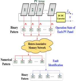
A photovoltaic array is a single electricity-producing unit in which several PV panel components are arranged in parallel (or in a series configuration) to increase output power. PV energy conversion systems use a solar tracking system with maximum power point tracking (MPPT) methods to improve output performance and battery charge solutions [1-3]. There are different sized PV systems, ranging from small, rooftop, or building-integrated systems with capacities >10 kilowatts to those with capacities of >100’s of megawatts in concentrated solar, heating/cooling systems, and home power supplies. A PV system can operate in grid-connected and off-grid modes within a smart grid or within a small portion of the electricity market. In Taiwan, PV systems have niche usages in outdoor spaces due to the subtropical environment, and they are easy to install and operate noiselessly. However, the output power of a PV system is influenced by changes in environmental conditions, such as solar radiation and temperature. In addition, output power may be affected by any fault within the PV array, such as grounded faults, open circuit faults, and bridged faults [4-6]. Power fuses, overcurrent protection devices, and grounded fault protection devices can be employed to isolate grounded faults on DC–DC converter sites and DC–AC inverter sites, but as fault currents are also affected by environmental conditions, protection devices are unable to clear the fault under low solar radiation or during night-to-day transition. When there is a lower output current, MPPT methods can interfere to estimate the output current while a certain fault is identified, thereby triggering the current-based protection device [6-7]. It is difficult to locate faults via manual inspection within a PV array; therefore an online assistant tool is necessary for use in locating multiple faults and conducting long-term outdoor monitoring. As output power is significantly altered by damage or faults occurring in one or more PV panels, this study thus proposes a bidirectional associative memory network to detect multiple faults within the PV array, as seen a schematic
2 diagram in Figure 1.
Manual techniques are traditionally used to examine PV panels, such as individual inspections, imaging examinations, and electrical examinations. In the laboratory or during manufacture quality control processing, visual inspection, thermal imaging analysis, and infrared thermography (IRT) are commonly used to observe color changes and visible hot spots on thermal images or the IRT of solar panels. These methods are safe and involve no-contact measurements to check the solar panels for open circuits/short circuits in a cell string, cell ruptures, and cell or/and glass cracks [8-10]. However, such examinations are only used to protect both the customer and the contractor before solar panel installation and require extra thermal imaging cameras or IRT to be mounted in front of the PV panel, and thus are usually used in the laboratory to identify designs, materials, and cell flaws (IEC 61215/IEC61646). To measure voltage and current on the DC–DC converter site or DC– AC inverter site, electrical examinations are needed; these are also required to determine and quantify output power degradation due to possible faulted panels in a PV array [6, 11-13]. It is known that any fault in an array can cause output power degradation, and thus conducting an electrical examination using current (I)-voltage (V) or V-power (P) curve analysis string by string is a reliable online testing method used to determine the locations of multiple faults.
Figure 1. Schematic diagram of multiple fault location in a PV array using hetero-associative memory network
On the DC–AC inverter side, the inverter has no overcurrent or overvoltage because a transformer provides galvanic isolation between the PV array and the utility grid. Power fuses, overcurrent, and ground-fault protection devices have been used to isolate ground faults in a conductor and any overcurrent from the PV array or fault on the grid-connected side. However, on the DC–DC converter side, the output power and currents can be degraded due to any fault within an array. Previous studies [6-7] have proposed that use of the MPPT algorithm may prevent faults during periods of lower solar radiation and night-to-day transition, as the algorithm can locate the reference value at the maximum power point. When the measured output power is degraded, based on the electrical property, faults such as grounded faults, line-to- line faults, and open circuit faults can be identified [6, 11-13].
Based on an electrical examination, this study proposes use of the bidirectional hetero-associative memory (BHAM) network [14-17] to detect multiple faults in a PV array. The BHAM network can store the training patterns in a connecting matrix when modeling the human cognitive process [16]. Its mechanism investigates various conditions represented by encoding weighted values in a weighting matrix; this process can maximize information representation and reduce memory requirements. In addition, BHAM is able to learn and recall various types of input and output associations. The proposed modified configuration with the hidden layer is used to solve nonlinear separable problems [14], and its manner can deal with inputs and outputs using binary,
. . .
PV Array
1
2
3
8
0/1 0/1 0/1
0/1 . . .
Hetero-Associative Memory Network
0/1 0/2 0/3 . . . 0/8
Binary
Pattern
Numerical
Pattern
0/1 0/1 0/1 . . . 0/1
Binary Pattern
Operation State of
Each PV Panel
Fault
Identification
DC-DC Converter V
p1
+
_
I
3
bipolar, or numerical data. Using nonlinear output feedback, it can also act using biological behavior in the form of hetero-associative memories for different data types and data lengths. The proposed model is also easily implemented in an embedded system or a tablet PC. Thus, experimental results show it is capable of detecting multiple faults in a rooftop PV system.
The remainder of this paper is organized as follows. Section 2 describes the methodology, including the maximum output power estimation, typical fault analysis in a PV array, and the BHAM network. Sections 3 and 4 present the simulation results and conclusion to demonstrate the efficiency of the proposed model in locating multiple faults.
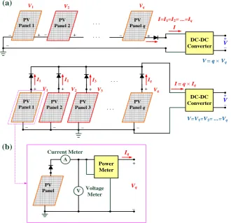
Figure 2. Schematic diagram of PV array. (a) PV array in a parallel or series configuration, (b) Measurement system of each PV panel
2. METHODOLOGY
2.1. Maximum Output Power Estimation and Fault Feature Extraction
PV panels are wired in a parallel or series configuration to form a PV array and increase output voltage or current (12/48 voltage). When wiring PV panels in a parallel configuration, the output amperage (current) is additive, I =qIq, where q is the number of PV panels in parallel, as seen in Figure 2(a). The output voltage, V, and current, I, for q PV panels in a parallel or series configuration can be expressed as
P a r a l l e l :
( 1 )
S e r i e s :
( 2 )
where IL is the grid rated load current; parameter, a, is the environment modified factor, and a = 7.8–9.0 in Taiwan; is the output effectiveness; Vq is the rated voltage per PV panel, Vq = 12 or 24 voltage; and s is the number of PV panels in a series. Thus, the output power can be increased, as
( 3 )
A MPPT algorithm, such as the incremental conductance method (ICM) [1-2] or ICM based method [3], is used PV
Panel
A
V Current Meter
Voltage Meter
Power Meter
Iq
+
_ Vq
(a)
(b)
PV Panel 1
+
_ PV Panel 2
+
_
I2 I1
I= q Iq
+ _
DC-DC Converter V
Iq
+
_ . . .
. . . PV
Panel 3 I3
+
V1 V2 V3
_
Vq
PV Panel q
V=V1=V2= ...=Vq
PV Panel 1
+ _ PV Panel 2
_
+ _
DC-DC Converter V
_
. . .
V1 Vq
PV Panel q
I=I1=I2= ...=Iq
. . .
+ +
V2
V= q Vq
I _
L
q I a I q
I=
q V s
V =
q q I V s q I V
4
to estimate the output power of each PV panel. If we suppose that the PV panels are wired in a parallel configuration, as seen in Figure 2(a), and that the electrical characteristics of the PV panels are identical, the estimated terminal voltage, Vq,est, and photo-current, Iph,q, of each PV panel are as follows,
( 4 )
( 5 )
( 6 )
where Isat is the reverse saturation current; T is the surface temperature of the cell; npand ns are the number of modules connected in parallel and series, respectively; Q is the electron charge; b is Boltzmann’s constant; A is the p–n junction ideality factor, which is typically in the range of 1<A <5 for different manufacturers; Tc is the ambient temperature; Tr is the reference temperature (25C); Isc is the cell short-circuit current at Tr; ksc is the short-circuit current temperature coefficient; S is the solar radiation; is the temperature compensation coefficient.
Therefore, the maximum output power (MOP) of each PV panel, Pq,est, and total MOP, Pest, can be
estimated as
( 7 )
( 8 )
The PV characteristics, such as power-voltage (P-V) and current-voltage (I-V) curves, vary widely depending on atmospheric conditions, such as solar radiation and temperature. Fault voltages, fault currents, and output power degradations are affected by fault types. Typical faults occurring in a PV panel include: (a) open circuit fault (OCF); (b) bridged (line-to-line) fault (BF); (c) and (d) lowerand upper grounded faults, respectively, (LGF/UGF) [6, 11-13]. When any fault occurs in a PV panel, voltage, current, and power meters can be employed to measure the output power, Pq,mea, of each panel, as seen in the measurement system in Figure 2(b).
The MPPT algorithm can be used to estimate the MOP. It is known that when measuring output power degradation, the measured value, and estimated value are not identical for given environmental conditions. Hence, the MOP is an important index from the viewpoint of fault identification. For each PV panel, this power index can be defined as
( 9 )
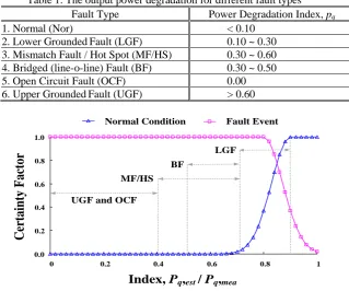
As shown in Table 1, it can be seen that the index, pq, of power degradations is computed in per-unit (pu) quantities with an interval of [0,1] and with an estimated output power, Pq,est. According to the power degradation of each PV panel, the index can be parameterized with certainty factors as
( 1 0 )
( 1 1 )
where q=0.10, q =1, 2, 3, …, n (n=8 means 8 PV panels in this study). The functions of certainty factors for normal condition and fault types are shown in Figure 3. The operation state of each PV panel can be identified as
( 1 2 )
The state vector S =[s1, s2, …, sq, …, sn]=[0/1, 0/1, …, 0/1, … , 0/1]. For n-digit binary numbers, each bit has
two states, {0, 1}, and the total number of the n-digit binary string is 2n combinations. Hence, with 8 PV panels ) ln( , sat p q sat p ph p s est q I n I I n I n Q bTA n
V = + −
100 )] ( [ , S T T k I
Iphq = sc+ sc c− r
) 25 (
, + −
= qest c
est V T
V q ph est q est
q V I
P, = , ,
est q est q P
P = ,
est q mea q
q P P
p = , ,
− − = 90 . 0 ), ) 90 . 0 ( 1 exp( 00 . 1 90 . 0 , 1 2 1 q q q q
q p p
p
− − = 80 . 0 ), ) 80 . 0 ( 1 exp( 80 . 0 00 . 0 , 1 2 2 q q q q q p p p = 1 2 1 2 , 0 , 1 q q q q q5
Table 1. The output power degradation for different fault types Fault Type Power Degradation Index, pq
1. Normal (Nor) < 0.10
2. Lower GroundedFault (LGF) 0.10 ~ 0.30 3. Mismatch Fault / Hot Spot (MF/HS) 0.30 ~ 0.60 4. Bridged (line-o-line) Fault (BF) 0.30 ~ 0.50
5. Open Circuit Fault (OCF) 0.00
6. Upper GroundedFault (UGF) > 0.60
Figure 3. The certainty factors versus the index, pq, for normal condition and fault types
in an array (n =8, q’=0,1, 2, …, n), we have 28 = 256 combinations of different binary patterns, as
,
( 1 3 )
( 1 4 ) Therefore, we have 256 binary patterns to represent the fault patterns. The corresponding binary patterns can
be encoded as binary values of 1 or 0, with the value “1” indicating a “PV fault”, and everything else can be encoded by the value “0.” A bidirectional associative memory network can thus be designed as a neuro-dynamic model to identify the faults within a PV array.
2.2. Bidirectional Associative Memory Network
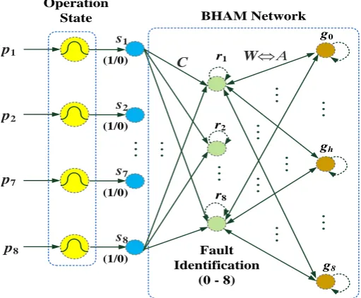
A recurrent memory network is an unsupervised dynamic learning system and can be classified into either auto-associative or hetero-associative memory models. A BHAM network is a feedback pattern mechanism that allows for the generation of new patterns, noise filtering, and pattern completion [14, 16]. It has a network that contains an input layer, output layer, and network connections, as shown in Figure 4. The network connections between the process units are bidirectional and in a loop configuration; this dynamic system can deal with binary and bipolar data, and can also represent biological behavior with both auto-associative and hetero-associative memories. Its multi-layer mechanism can generate output patterns using nonlinear output feedback, such as Gaussian functions, and can also associate different data types (numerical data) or data lengths (output vector). The machine learning algorithm stores information and matrices using noise-free versions of the input and output patterns. Given 8 PV panels in an array, the BHAM algorithm has two stages, t h e l e a r n i n g s t a g e a n d t h e r e c a l l i n g stage, as delineated below.
Learning stage
Step 1) establish the input-output pair of the training pattern, Sk and Rk, k = 1, 2, 3, …, K, K =256 binary training patterns, where state vector, Sk = [sk1,…, ski, …, skn]t, ski {0, 1}, and the fault pattern, Rk = [rk1, …,
rkj, …, rkn]t, Rkj {0, 1}.
Step 2) establish the connecting matrix C using K pairs of training patterns,
0.0 0.2 0.4 0.6 0.8 1.0
0 0.2 0.4 0.6 0.8 1
C
er
ta
in
ty
F
ac
to
r
Index, Pq,est / Pq,mea LGF
MF/HS BF
UGF and OCF
Normal Condition Fault Event
)! ' 8 ( ! '
! 8 '
8
q q
q = −
1 8 8
0 8
= =
= =
= − =
= n
q
n
q q
q q
q n N
0
' ' 0
' 256
)! ' 8 )( ! ' (
6
( 1 5 ) where C = [wij]n n.
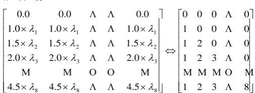
Step 3) find n eigenvalues, i = wij, i =j = 1, 2, 3, … , 8, the weight matrix, W, and the associative matrix, A, for the eight faults as following
( 1 6 )
( 1 7 )
( 1 8 )
where h, h=0, 1, 2, …, 8, is the weight value for normal condition and eight faults within the weight matrix, W =[hi]9 8, hi =hi, and each element in the associative matrix, A = [ahj]9 8, element, ahj, is encoded as
numerical data from value “1” to value “8” to indicate which one is fault in a PV array, and the normal condition is encoded as the value “0.”
Figure 4. The configuration of BHAM network
Recalling stage
Step 1) obtain the network connecting matrices, C, W, and A, and apply the testing pattern S0 =[s1, s2, … , si, …,
s8] to the BHAM network;
Step 2) associate the output pattern, R0 = [r1, r2, … , ri, …, r8]T, as
=
= K k
t k R S C 1 k A W = 8 8 5 8 8 1 8 8 5 5 5 2 5 1 5 8 1 5 1 2 1 1 1 8 0 5 0 2 0 1 0 W = 8 7 6 5 4 3 2 1 0 0 0 0 4 3 2 1 0 0 0 0 0 0 0 1 0 0 0 0 0 0 0 0 A s1 s2 s7 s8 . . . BHAM Network (1/0) (1/0) (1/0) (1/0) r1 r2 r8 . . . . . . . . . . . .
WA
C g0 gh g8 . . . . . . . . . Operation State . . . . . . Fault Identification
(0 - 8)
p1
p2
p7
7
, , i = 1 , 2 , 3 , … , 8
( 1 9 )
Step 3) transit the output pattern, R0, to the Gaussian function unit, gh, and the output of gh, as
, h=0, 2, 3, … , 8 (20)
| | h i – r i | |
( 2 1 )
where is the standard deviation, = min(EDh)0.90; if the pattern, R0, is similar to any row weight vector of
matrix W, the EDh will be small (EDh → 0, argmin||EDh||, h = 0, 2, 3, …, 8) and the gh unit will approach 1. The gh unit is the index that measure the similarity degree among nine row weight vectors;
Step 4) transit the outputs of the gh units to the ri unit with nonlinear feedback and compute the output of the ri unit using the hard limit function with a threshold value of 0.50, as
( 2 2 )
R0p=[r1, r2,…, ri, …, r8], , i=1, 2, 3, …, 8 (23)
Step 5) transit bidirectional patterns repeatedly between the ri units and gh units until bidirectional stability is reached. When the patterns, R0, is not changed, and , where p is the iteration
number, then the BHAM algorithm will be terminated.
When the BHAM network reaches bidirectional stability, the state si = 1, means one or more faults have been detected. Thus, the BHAM network associates the numerical data to locate which PV panel is at fault within the PV array. A flow chart of the BHAM algorithm for multiple fault location is shown in Figure 5.
0
0 C S
R = T
=
= 8
1
i i ji i w s r
) ) ( 2
1
exp( 2
2 h
h ED
g = −
= − = 8
1
2
) (
i
i hi
h r
ED
=
50 . 0 , 0
50 . 0 , 1
'
h h
h g
g g
== 9
1 '
h h ih
i a g
r
0 || || 0 0 1
0 = − =
8
Figure 5. The flow chart of fault location and BHAM algorithm 3. EXPERIMENTAL RESULTS AND DISCUSSION
The proposed multiple fault location algorithm using a BHAM network was designed and tested on a PC Pentium-IV 2.4 GHz with 480 MB RAM and MATLAB mathematical computing software (MathWorks, Natick, Massachusetts, USA). Relevant specific parameters of each PV panel used in this study are shown in Table 2. In Taiwan’s subtropical outdoor environment, the average solar radiation and temperature are approximately 0.20–0.80 kW/m2 and 30–40°C, respectively, during the summer season. For various radiation and temperature
values, the MPPT algorithm [1-3, 18-19] can be employed to control the DC–DC boost converter until the desired MOP and output voltage is reached. In this study, an ICM based method [1, 3] is used to estimate the desired output and adjust the boost converter’s duty ratio to match the maximum point. The MPPT is used to track the MOP by adjusting the voltage as solar radiation and temperature increase from 0.2 kW/m2 to 1.0
kW/m2 and from 30°C to 45°C, respectively. The P–V and the I–V characteristic curves of each PV panel are
shown in Figure 6. Hence, when atmospheric conditions change, the MPPT algorithm takes less than 10 switching controls to achieve the desired value. During the summer season, each PV panel had output powers of 199.1W to 262.2W, output currents of 9.8A to 13.6A, and an output voltage of 19.8V, as seen in Figures 6(a) and 6(b). The boost converter adjusts the duty ratio until the desired values of output power and voltage are reached, as seen in Figure 6(c). The experimental results confirm that the MPPT can estimate the output power of each panel under various atmospheric conditions, and it can also work during low solar radiation and at the night-to-day transition.
Table 2. Specific parameters of each PV panel (at solar radiation of 1.0kW/m2 and a temperature of 25C) [1,
3]
Specific Parameter Value
Maximum Power Pmax 87.70 (W)
Short-circuit Current ISC 4.80 (A)
Open-circuit Voltage VOC 21.70 (V)
Estimate the MOP of each PV panel using MPPT algorithm
Apply the testing pattern, S0, to the
connecting network
Start
End
Transit the output pattern, R0, to the
Gaussian function unit, gh Associate the output pattern, R0
Establish Network Connecting Matrices, C, W, and A
Identify the states, si, i=1, 2, …, 8, of PV panels using equations, (10) to (12)
Matrix, C
Matrix, W
Compute the output of Gaussian function using the hard limit function
Transit the outputs of gh units to the ri unit
Matrix, A
Bidirectional Stability ?
Yes
No
(1) Learning Sage
(2) Recalling stage
Obtain the meter-reading power
9
Rated Voltage VR 19.14 (V)
Rated Current IR 4.58 (A)
Number of Modules Connected in Series ns 36 Number of Modules Connected in Parallel np 2
Table 3. Specific parameters of a rooftop PV system with two strings in summer season String Panel
Number
Radiation kW/m2
Temperature
°C Each Panel Power (W)
Total Output Power (kW) and Current (A)
1# 8 0.2 – 1.0 30 – 45 199.1-262.2 1.6 – 2.1 kW
78.4 – 108.8 A
2# 8 0.2 – 1.0 30 – 45 199.1-262.2 1.6 – 2.1 kW
78.4 – 108.8 A
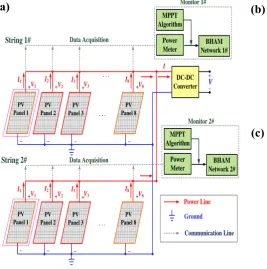
For a rooftop PV system, we built an array of about 3.2–4.2 kW PV in the summer season, which consists of two strings with 16 identical PV panels in parallel (the same manufacturer), as shown in the experimental setup in Figure 7(a). The specific parameters of the rooftop PV system with two strings (1# and 2#) in the summer season are shown in Table 3. The measurement system includes voltage, current, and power collected through data acquisition meters and ommunication lines. Two BHAM networks are employed to locate PV panels with faults. The times between 08:00 and 18:00 was divided into 40 time slots (15 min time slots) for monitoring the rooftop PV system. Atmospheric conditions are shown in Figure 7(b), and each of the PV panels, string measurements, and estimation powers are shown in Figure 7(c). The total string output power was 2.87– 3.44 kW and the output power of each panel was 0.18–0.23 kW. In addition, each BHAM network had eight input nodes, nine hidden nodes, and 8 output nodes. The total memory storage for the connecting matrix, C (8 8), weight matrix, W (89), and associative matrix, A (89), is 832 bytes (208×4 bytes). The weight matrix, W, and associative matrix, A, are
where elements, 1=2=…=8=128, are eigenvalues of matrix C.
10
Figure 6. The MPPT estimated results. (a) Output power versus output voltage, (b) Output current versus output voltage, (c) Duty ratio versus switch number
0 5 10 15 20 25
0 5 10 15
1 2 3 4 5 6 7 8 9 10
0.0 0.5 1.0
(1) (2) (3) (4)
T=45°, S=1.0kW/m2 T=40°, S=0.8kW/m2
T=35°, S=0.4kW/m2
T=30°, S=0.2kW/m2
0 5 10 15 20 25
0 100 200 300
262.2W 230.8W 199.1W 199.1W (1)
(2) (3) (4) (1)
(2) (3) (4)
T=45°, S=1.0kW/m2 T=40°, S=0.8kW/m2
T=35°, S=0.4kW/m2 T=30°, S=0.2kW/m2
13.6(A) 11.9(A) 10.4(A) 9.8(A) (1)
(2) (3) (4)
19.8(V)
(a)
(b)
O
u
tp
u
t
P
ow
er
(
W
)
Output Voltage (V)
Output Voltage (V)
O
u
tp
u
t
C
u
rr
en
t
(A
)
(c)
D
u
ty
R
at
io
Switch Number
PV Panel 1
+
_
PV Panel 2
+
_
+ _ DC-DC Converter V
I8
+
_ . . .
. . .
PV Panel 3
+
V1 V2 V3
_
V8
PV Panel 8
I1 I2 I3
PV Panel 1
+
_
PV Panel 2
+
_
I8
+
_ . . .
PV Panel 3
+
V1 V2 V3
_
V8
PV Panel 8
I1 I2 I3
I
String 1#
String 2#
Power Meter
BHAM Network 1# MPPT
Algorithm
Power Meter
BHAM Network 2# MPPT
Algorithm Monitor 1#
Monitor 2#
Power Line
Ground
Communication Line
Data Acquisition
Data Acquisition
(a)
(b)
11
Figure 7. Experimental setup. (a) Schematic diagram of a rooftop PV system, consisting of 2 strings with 16 PV panels; (b) Solar radiation and temperature versus time (from 8:00 a.m. to 18:00 p.m.); (c) Each PV panel and string measurement power and estimation power
If we assume that multiple open circuit faults occurred in PV panels, 1#, 2#, and 3# at string 1#, and in PV panels, 1#, 2#, and 3# at string 2#; therefore output power was not generated. At 13:00, solar radiation and temperature were 830 kW/m2 and 37.5°C; the MPPT algorithm was employed to estimate the MOP, 224.4W,
for each PV panel, and the output power for each faulted panel was 0.0W. Six of the PV panels in parallel were disconnected, and thus the string output power degraded 37.5% of the MOP and an overcurrent was not generated. Hence, 16 power indexes could be estimated using Equation (9). The fault location procedures at the recall stage for two BHAM networks are as follows:
Step 1) String 1#: [p1, p2, p3, p4, p5, p6, p7, p8]=[0.00, 0.00, 0.00, 0.95, 0.96, 0.95, 0.96, 0.97];
String 2#: [p1, p2, p3, p4, p5, p6, p7, p8]=[0.00, 0.00, 0.00, 0.96, 0.97, 0.96, 0.96, 0.95];
Step 2) power indexes were parameterized using equations, (10) to (12). The operation states of 16 PV panels were identified as
String 1#: [s1, s2, s3, s4, s5, s6, s7, s8]=[1, 1, 1, 0, 0, 0, 0, 0];
String 2#: [s1, s2, s3, s4, s5, s6, s7, s8]=[1, 1, 1, 0, 0, 0, 0, 0];
Step 3) associated the output patterns:
String 1#: [r1, r2, r3, r4, r5, r6, r7, r8]=[256, 256, 256, 192, 192, 192, 192, 192];
String 2#: [r1, r2, r3, r4, r5, r6, r7, r8]=[256, 256, 256, 192, 192, 192, 192, 192];
Step 4) computed the outputs of Gaussian function units:
String 1#: [g1, g2, g3, g4, g5, g6, g7, g8]=[0.0454, 0.2665, 0.5738, 0.4881, 0.2148, 0.0888, 0.0362, 0.0147,
0.0060];
String 2#: [g1, g2, g3, g4, g5, g6, g7, g8]=[0.0454, 0.2665, 0.5738, 0.4881, 0.2148, 0.0888, 0.0362, 0.0147,
0.0060];
Step 5) transited the outputs of Gaussian function units to the output units using equations, (22) and (23): String 1#: [r1, r2, r3, r4, r5, r6, r7, r8]=[1, 2, 3, 0, 0, 0, 0, 0];
String 2#: [r1, r2, r3, r4, r5, r6, r7, r8]=[1, 2, 3, 0, 0, 0, 0, 0];
Step 6) reached bidirectional stability and terminated the BHAM algorithm.
In addition, from 08:00 to 18:00, 41 experimental tests were conducted, and the results of fault locations indicated normal operating conditions from 8:00 to 12:45, 6 PV panels with faults between 13:00 and 16:30, and 8 PV panels with faults from 16:45 to 18:00. The experimental results indicate a fault location accuracy of 100% (hit rate). Experimental results confirmed that the proposed model enables accurate multiple fault location within the PV array.
Therefore, by using electrical examinations these promising results could be given to operators prior to performing visual inspections using thermal sensors or IRTs. In solar panel maintenance, visual inspections
0 5 10 15 20 25 30 35 40
8 8.5 9 9.5 10 10.5 11 11.5 12 12.5 13 13.5 14 14.5 15 15.5 16 16.5 17 17.5 18 0 100 200 300 400 500 600 700 800 900
0 50 100 150 200 250
8 8.5 9 9.5 10 10.5 11 11.5 12 12.5 13 13.5 14 14.5 15 15.5 16 16.5 17 17.5 180 500 1000 1500 2000 2500 3000 3500 4000
Time (Hour)
Time (Hour)
T
e
m
p
e
r
a
tu
r
e
(
°
C
)
R
a
d
ia
ti
o
n
(
k
W
/m
2)
E
a
c
h
P
a
n
e
l
O
u
tp
u
t
P
o
w
e
r
(W
)
S
tr
in
g
O
u
tp
u
t
P
o
w
e
r
(W
)
Each Panel Measurement Power Each Panel Estimation Power String Estimation Power
String Measurement Power with Panel Faults Temperature (°C)
12
could thus be conducted to check for defects in any of the panels. In addition, drone/light unmanned vehicle techniques with infrared cameras could also be instead of ground-based inspection techniques [20-22]. Furthermore, pilot and sensor operator inspected visual images can be taken from a height of 10-15m during maintenance in a large-scaled PV system or rooftop system, which could reduce the number of manual tasks required and reduce the amount of time taken to conduct the inspections. Therefore, maintenance engineers could visit fault locations without the need to survey the entire PV array, which could ultimately reduce operating costs. Faults types could be rapidly examined using manual and drone inspections, which would reduce the need for online examinations; electrical examinations and unmanned technology could thus be integrated into inspections, thereby reducing costs and time.
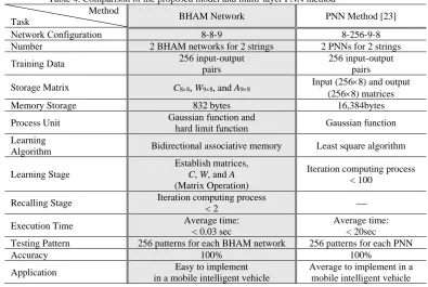
To compare the proposed machine learning model with other intelligent methods, we used the same 256 input-output pairs of training data to train an artificial neural network, where 256 training patterns were used to determine the configuration of probability neural network (PNN) [23]. The multi-layer PNN consists of an input layer with 8 input nodes, a pattern layer with 256 nodes, and an output layer with eight nodes. Optimal PNN parameters were determined using the traditional least-square algorithm or the gradient descent algorithm [24-25]. For the pre-specified tolerance value with mean squared error, 10−2
, the iteration computingprocess
took about <100 iterative computations to reach the convergent condition.However, initial condition assignments, such as initial network parameters and learning rates, can affect the model’s learning outcome performance. In addition, fill-in with elementsin the input and output matrices can increase computing time and memory storage requirements. Therefore, considering 4 bytes for digital storage, the total memory storage was 16,384 bytes (input matrix: 25684 bytes and output matrix: 25684 bytes). PNN also provided a 100% hit rate and provided promising results for detecting multiple fault locations. However, in contrast to the proposed model, the iterative computing processes and memory storage requirements had two limitations.
Although the proposed model showed a very fast training and recalling processes, its memory storage requirement needs to be reduced, as shown in Table 4. the proposed model is easy to implement in portable device designs, such as intelligent mobile vehicles or drone /light unmanned vehicles. The measurement system transited metering PV panels’ output powers to a mobile vehicle via WiFi wireless communication (IEEE 802.11 standards wireless local area network, WLAN) [26]. Thus, the reliable of location and detection results
c o u l d b e
enhanced.
Table 4. Comparison of the proposed model and multi-layer PNN method Method
Task BHAM Network PNN Method [23]
Network Configuration 8-8-9 8-256-9-8
Number 2 BHAM networks for 2 strings 2 PNNs for 2 strings
Training Data 256 input-output
pairs
256 input-output pairs
Storage Matrix C88, W98, and A98 Input (2568) and output
(2568) matrices
Memory Storage 832 bytes 16,384bytes
Process Unit Gaussian function and hard limit function Gaussian function
Learning
Algorithm Bidirectional associative memory Least square algorithm
Learning Stage
Establish matrices, C, W, and A (Matrix Operation)
Iteration computing process < 100
Recalling Stage Iteration computing process
< 2 ⎯
Execution Time Average time:
< 0.03 sec
Average time: < 20sec
Testing Pattern 256 patterns for each BHAM network 256 patterns for each PNN
Accuracy 100% 100%
Application Easy to implement
in a mobile intelligent vehicle
Average to implement in a mobile intelligent vehicle
4. CONCLUSION
13
without updating network parameters. It took approximately <0.03 sec to complete the recall stage. It is considered that this method can overcome the complexity involved in an adjustable pattern mechanism. The matrix and logic operations require only a short design cycle, and it is easily implemented in a portable embedded system or a mobile intelligent vehicle. In addition, as the capacity of PV systems will increase when connecting several PV panels in either parallel or series, and this will use a vast amount of space and long-term outdoor operations, the promising technology presented here can be integrated into light unmanned vehicles and wireless communication. In addition, through an advanced metering infrastructure, metering power data can be transited to the a BHAM based monitor via WiFi wireless. Results show that the proposed method uses a short examination time and is highly accurate.
Acknowledge: This work is supported in part by the Ministry of Science and Technology, Taiwan, under contract number: MOST 105-2634-F-244-001, duration: November 1, 2016~October 31, 2017.
Author Contributions: The model analysis on the multiple fault location in a photovoltaic array was made by Long-Yi Chang, Neng-Sheng Pai, and Min-Hung Chou. The model algorithm was designed by Chia-Hung Lin, Jian-Liung Chen, and Chao-Lin Kuo, and also carried out the simulations and experiments. Long-Yi Chang was responsible for writing the paper and serves as the corresponding author.
Conflicts of Interest: The authors declare no conflict of interest
REFERENCE
[1] Chia-Hung Lin, Cong-Hui Huang, Yi-Chun Du, and Jian-Liung Chen, “Maximum photovoltaic power tracking for the PV array using the fractional-order incremental conductance method, ”Applied Energy, vol. 88, no. 12, pp. 4840-4847, December 2011.
[2] Chian-Song Chiu and Ya-Lun Ouyang, “Robust maximum power racking control of uncertain photovoltaic systems: a unified T-S Fuzzy model-based approach, ”IEEE Transactions on Control Systems Technology, vol. 19, no. 6, November 2011, pp. 1516-1526.
[3] Chao-Lin Kuo, Chia-Hung Lin, Her-Terng Yau, and Jian-Liung Chen, “Using self-synchronization error dynamics formulation based controller for maximum photovoltaic power tracking in micro-grid systems, ”IEEE Journal on Emerging and Selected Topics in Circuits and Systems, vol. 3, no. 3, September 2013, pp. 459-467.
[4] Kuei-Hsiang Chao, Bo-Jyun Liao, and Chin-Pao Hung, “Applying a cerebellar model articulation controller neural network to a photovoltaic power generation system fault diagnosis,” International Journal of Photoenergy, vol. 2013, Article ID 839621, 12 pages.
[5] Ye Zhao, Fault analysis in solar photovoltaic arrays, Electrical and Computer Engineering Master’s These, Northeastern University, December, 2010.
[6] Chao-Lin Kuo, Jian-Liung Chen, Shi-Jaw Chen, Chih-Cheng Kao, Her-Terng Yau, and Chia-Hung Lin, “Photovoltaic energy conversion system fault detection using fractional-order color relation classifier in micro-distribution systems, ”IEEE Transactions on Smart Grid, Article in Press, April 2016, DOI: 10.1109/TSG.2015.2478855.
[7] Y. Zhao, B. Lehman, J. F. DePalma, J. Mosesian, and R. Lyons, “Fault evolution in photovoltaic array during night-to-day transition, ”2010 IEEE 12th Workshop on control and Modeling for Power Electronics,
2010, pp. 1-6.
[8] Testo, Inc., Practical guide: solar panel thermography, www.testo..com.
[9] E. Kaplani, “Detection of degradation effects in field-aged c-Si solar cells through IR thermography and digital image processing, ”International Journal of Photoenergy, vol. 2012, Article ID 396792, 11 pages. [10] Kumar Suresh, Sarkar Bijan, and K. S. Nija, “Quality improvement of PV modules by electroluminescence
and thermal Imaging, ”International Journal of Engineering and Advanced Technology, vol. 3, no. 3, February 2014, pp. 422-427.
[11] Jian-Liung Chen, Chao-Lin Kuo, Shi-Jaw Chen, Chih-Cheng Kao, Tung-Sheng Zhan, Chia-Hung Lin, and Ying-Shin Chen, “DC-side fault detection for photovoltaic energy conversion system using fractional-order dynamic error based fuzzy Petri net integrating with intelligent meters, ”IET-Renewable Power Generation, vol. 10, no. 9, 2016, pp. 1318-1327.
14
[13] Mehrdad Davarifar, Abdelhamid Rabhi, and Ahmed El Hajjaji, “Comprehensive modulation and classification of faults and analysis their effect in DC side of photovoltaic system,” Energy and Power Engineering, vol. 2013, no. 5, July 2013, pp. 230-236.
[14] Sylvain Chartier and Mounir Boukadoum, “A bidirectional heteroassociative memory for binary and grey-level patterns, ”IEEE Transactions on Neural Networks, vol. 17, no. 2, 2006, pp. 385-396.
[15] Zixing Zhang, Joel Pinto, and Christian Plahl, “Channel mapping using bidirectional long short-term memory for dereverberation in hands-free voice controlled devices, ”IEEE Transaction on Consumer Electronics, vol. 60, no. 3, August 2014, pp. 525-533.
[16] Nareg Berberian, Zoya Aamir, and Sebastien Helie, “Encoding sparse features in a bidirectional associative memory,” 2016 International Joint Conference on Neural networks, July 2016.
[17] Dapeng Tao, Yonggang Wen, and Richang Hong, “Multicolumn bidirectional long short-term memory for mobile devices-based human activity recognition, ”IEEE Internet of Things Journal, vol. 3, no. 6, December 2016, pp. 2327-1134.
[18] A. Pandey, N. Dasgupta, and A. K. Mukkerjee, “High- performance algorithms for drift avoidance and fast tracking in solar MPPT system, ”IEEE Transactions on Energy Conversion, vol. 23, no. 2, pp. 681-689, June 2008.
[19] C. A. Otieno, G. N. Nyakoe, and C. W. wekesa “A neural Fuzzy based maximum power point tracker for a photovoltaic system, ”2009 IEEE AFRICON, Nairobi, Kenya, 23-25 September, pp. 1-6, 2009. [20] Claudia Buerhop, Tobias Pickel, and Manuel Dalsass, “Air-PV-check: a quality inspection of PV-power
plants without operation interruption,” 2016 IEEE 43rd Photovoltaic Specialists Conference, June 2016.
[21] M. Aghaei, A. Dolara, and S. Leva, “Image resolution and defects detection in PV inspection by unmanned technologies,” 2016 Power and Energy Society General Meeting, July 2016.
[22] Paolo Bellezza Quater, Francesco Grimaccia, and Sonia Leva, “Light unmanned aerial vehicles (UAVs) for cooperative inspection of PV plants,” IEEE Journal of Photovoltaics, vol. 4, no. 4, 2014, pp. 1107-1113.
[23] D. F. Specht, “A general regression neural network, “IEEE Trans. on Neural Network, 1991, pp. 568-576.
[24] J. X. Wu, C. H. Lin, Y. C. Du, and T. Chen, “Sprott chaos synchronization classifier for diabetic foot peripheral vascular occlusive disease estimation, ”IET Science, Measurement & Technology, vol. 6, no. 6, November 2012, pp. 533-540.
[25] Cong-Hui Huang, Chia-Hung Lin, and Chao-Lin Kuo, “Chaos- synchronization based detector for power quality disturbances classification in a power system, ”IEEE Transactions on Power Delivery, vol. 26, no. 2, 2011, pp. 944-953.
![Table 2. Specific parameters of each PV panel (at solar radiation of 1.0kW/m2 and a temperature of 25C) [1, 3]](https://thumb-us.123doks.com/thumbv2/123dok_us/1037671.1603994/8.595.131.468.66.446/table-specific-parameters-pv-panel-solar-radiation-temperature.webp)