Characterization of Necking Phenomena in High-Speed Experiments by Using a Single Camera

doi:10.1155/2010/215956

Research Article

Characterization of Necking Phenomena in High-Speed

Experiments by Using a Single Camera

Gilles Besnard,

_{Jean-Michel Lagrange,}

_{Franc¸ois Hild,}

_{St´ephane Roux,}

and Christophe Voltz

1_{CEA, DAM, DIF, 91297 Arpajon, France}

2_{LMT-Cachan, ENS Cachan/CNRS / UPMC, UniverSud Paris 61, avenue du Pr´esident Wilson, 94235 Cachan Cedex, France} 3_{CEA, DAM, 21120 Is-sur-Tille, France}

Correspondence should be addressed to Franc¸ois Hild,[email protected]

Received 6 January 2010; Accepted 24 June 2010

Academic Editor: Pascal Frossard

Copyright © 2010 Gilles Besnard et al. This is an open access article distributed under the Creative Commons Attribution License, which permits unrestricted use, distribution, and reproduction in any medium, provided the original work is properly cited.

The purpose of the experiment described herein is the study of material deformation (here a cylinder) induced by explosives. During its expansion, the cylinder (initially 3 mm thick) is thinning until fracture appears. Some tens of microseconds before destruction, strain localizations occur and induce mechanical necking. To characterize the time of first localizations, 25 stereoscopic acquisitions at about 500,000 frames per second are used by resorting to a single ultra-high speed camera. The 3D reconstruction from stereoscopic movies is described. A special calibration procedure is followed, namely, the calibration target is imaged during the experiment itself. To characterize the performance of the present procedure, resolution and optical distortions are estimated. The principle of stereoscopic reconstruction of an object subjected to a high-speed experiment is then developed. This reconstruction is achieved by using a global image correlation code that exploits random markings on the object outer surface. The spatial resolution of the estimated surface is evaluated thanks to a realistic image pair synthesis. Last, the time evolution of surface roughness is estimated. It gives access to the onset of necking.

1. Introduction

For detonics applications, objects subjected to very high deformations (about 50% to 100% strains) are to be observed in very short times (i.e., less than 100μs). To characterize the phenomenon of necking and to compare experimental results with hydrodynamic computations, ultra-fast cine-matography is very useful. This diagnostic, which is resolved in space and time, is used to monitor external surfaces of expanding objects. For the present applications, dedicated cameras are used [1]. Thanks to a stereoscopic setup, 3D reconstructions are possible.

The stereovision technique is used for mechanical obser-vations. Numerous applications exist for quasistatic experi-ments [2–5] where stereovision is coupled with digital image correlation [6]. The latter is a nonintrusive measurement technique that provides a large density of measurement points. Thanks to the generalization of digital cameras (with CCD or CMOS sensors), the use of stereo-correlation tends

is presented. A synthetic case is analyzed to determine the detection resolution (i.e., the minimum defect size). Last, in order to improve the quality of the 3D reconstruction, a correction method which allows for large displacements is presented. The whole procedure is finally illustrated to analyze a true experiment.

2. Stereovision Principle

This first part deals with the reconstruction of an object based upon stereoscopic observations. The principle of formation of images via mirrors and a rotating mirror framing camera and its calibration are introduced. The specific global digital image correlation algorithm used to perform stereomatching is finally presented.

2.1. Formation of Images via Mirrors. Mirrors are very useful tools in the field of vision and their shape can be designed to meet various specifications [11–13]. Several angles of view with the samecamera are possible. In this part, theoretical expressions of the transformation matrix, that is, relating the 3D coordinates of a point of the scene and its projection in the image plane are recalled. This is performed within the framework of an orthographical model with mirror, which is an appropriate model for the measurements performed herein since the object size is very small (height: 100 mm, diameter: 100 mm, see Figure1(a)) in comparison with the distance between the camera and the object (ca. 16 m).

Because of the large optical path between the camera and the object (about 16 m), image formation is split into two stages, illustrated in two dimensions in Figure1(a). This process is identical for the two mirrors and only the generic case is considered in the sequel. LetQbe a point in the image scene. It is imaged at pointQby mirror (P). The orthogonal projection ofQonto the image plane is denoted byq.

To establish the relationship in a 3D setting, the various transformations depicted in Figure 2 are considered. The reference frame of the scene is related to that of the image. LetΩbe the origin in the image plane. For any pointM,xM

denotes the vector position in the image frame. The mirror is defined by its normalnand its centerO. The mirror plane (P) is defined by the following equation for any point M

belonging to the mirror:

n·(xM−xO)=nxM+d=0 (1)

withd= −n·xO.

PointQis the orthogonal projection ofQon (P), so that

xQ−x_Q=kn, ₍₂₎

wherekis the distanceQQ

k= −n·xQ+d

. (3)

PointQis the symmetric ofQwith respect to plane (P) and its position is given by

xQ =xQ−2

n·xQ+d

n. (4)

Using homogeneous coordinates, the above relationship can be written in a matrix form

⎛ ⎜ ⎝ xQ yQ 1 ⎞ ⎟ ⎠= ⎡ ⎢ ⎣

−2n2

x −2nxny −2nxnz −2nxd −2nxny −2n2y −2nxnz −2nyd

0 0 0 1

⎤ ⎥ ⎦ ⎛ ⎜ ⎜ ⎜ ⎝ xQ yQ zQ 1 ⎞ ⎟ ⎟ ⎟ ⎠ ≡P ⎛ ⎜ ⎜ ⎜ ⎝ x y z 1 ⎞ ⎟ ⎟ ⎟ ⎠. (5)

The transformation from the mirror image to the camera is a classical problem [11]. Usually, it is decomposed into three elementary operations [14], namely, a projection matrixPassociated with the orthographic projection model

P= ⎡ ⎢ ⎣

π 0 0 0

0 π 0 0

0 0 0 1

⎤ ⎥

⎦, (6)

whereπis the magnification coefficient, matrixKis express-ing the transformation between the retinal coordinates in the retinal plane of the camera (in metric units) and the pixel coordinates in the image, and matrixAis associated with the transformation between the camera coordinate system and the reference coordinate system, attached to the object in the present case A= ⎡ ⎢ ⎢ ⎢ ⎣

r11 r12 r13 tx r21 r22 r23 ty r31 r32 r33 tz

0 0 0 1

⎤ ⎥ ⎥ ⎥

⎦, K= ⎡ ⎢ ⎣

ku 0 u0 0 kv v0

0 0 1

⎤ ⎥ ⎦, (7)

wherekuandkvare scale factors (horizontally and vertically

andri j andtkare rotation and translation parameters). The

combination of these matrices yields

⎛ ⎜ ⎝ u v 1 ⎞ ⎟ ⎠=KPA

⎛ ⎜ ⎜ ⎜ ⎝ X Y Z 1 ⎞ ⎟ ⎟ ⎟ ⎠ (8)

with (X,Y,Z, 1) being the homogeneous coordinates ofQin the reference frame. Last, the sought relationship reads

⎛ ⎜ ⎝ u v 1 ⎞ ⎟ ⎠= ⎡ ⎢ ⎣

m11 m12 m13 m14

m21 m22 m23 m24

0 0 0 1

⎤ ⎥ ⎦ ⎛ ⎜ ⎜ ⎜ ⎝ X Y Z 1 ⎞ ⎟ ⎟ ⎟ ⎠≡M

⎛ ⎜ ⎜ ⎜ ⎝ X Y Z 1 ⎞ ⎟ ⎟ ⎟ ⎠, (9)

where the parameters mi j denote the coefficients of the

transformation matrix M, whose expression is simplified compared with those obtained in the case of pinhole model [6]. In the present case,m3i =0 fori=1, 2, 3 andm34 =1 [14].

(a)

Q(x,y,z) Q

r Q

l

Q r Q

l

qr

ql Left image_plane

Right image plane

Mirror

Mirror

(b)

Figure1: Visualization of the stereoscopic system (a). Reference mirrors in which the cylinder and the calibration target can be seen. Above the mirrors, the pyrotechnic flashes are located in wood cases. Model of image formation in the case of two mirrors of reference and with an orthographic model (b).

Q Q

Q n

Zim Yim _Xim

Image frame

O

Z

X Object

frame

Im age

plane

Y

Mirror (P)

q

Figure2: Model of image formation via a mirrorPof normaln.

designed with a collection of known reference points xα

whereα = 1,. . .,N whose position is determined by using a coordinate measuring machine and an optical microscope leading to a 10μm uncertainty. Their image coordinatesuα

are identified. The relationship uα _{= Mx}α _{is exploited to}

determineMusing a least squares optimization strategy. The objective function to minimize is defined as

O(M)=

α

Mxα_−uα2

(10)

enforcing the conditionm34=1 [14].

Introducing matrixΞi j=xαixαj, the elements of matrixM

read

mi j=(Ξ)−ik1.

xα kuαj

. (11)

The expected conditionsm3i=0 fori=1−3 can be checked

as a self-consistent validation of the calibration. It is worth noting that with the model used herein, the coefficients

m31,m32, andm33are vanishingly small.

In practice, the calibration is carried out by putting a 3D target near the observed object (Figure3). The calibration using a planar object successively positioned at various

positions [15] is not possible in the present experiment. Only one image is necessary to calibrate the system. This approach (i.e., in situ calibration target) is implemented since lighting is obtained by pyrotechnic flashes that are only used during the experiment itself. The latter further requires that the explosive be introduced only at the very end of the experiment preparation, for safety reasons. Prior to that, the position of various objects (the mirrors in particular) may change slightly because of operator manipulations. Therefore, the calibration target has to remain in the field of view (and hence will be destroyed during the explosion). Therefore, the proposed camera calibration procedure is not “optimal” in the sense that all the field of view is not calibrated. However, it will be shown in Section4.2that the distortions remain small, thereby only having a small impact on the quality of the reconstruction.

Once the calibration has been carried out, the coordi-nates of the considered point in the 3D object frameXt ₌

(X,Y,Z) are overdetermined by the corresponding left and right image coordinatesUt _{= (u}

l,vl,ur,vr). A least squares

minimization is used to relateXtoU, which is written as

X=(CtC)−1Ct(U−D) (12) with

C= ⎛ ⎜ ⎜ ⎜ ⎝

ml

11 ml12 ml13

ml21 ml22 ml23

mr11 mr12 mr13

mr21 mr22 mr23

⎞ ⎟ ⎟ ⎟

⎠, D= ⎛ ⎜ ⎜ ⎜ ⎝

ml

14

ml24

mr14

mr24

⎞ ⎟ ⎟ ⎟

⎠, (13)

whereml

i j (resp.,mri j) are the coefficients of the left (resp.,

right) transformation matrix.

(a) (b)

Figure3: Calibration target (a) and its positioning on the experimental stage (b). The centers of the white squares are automatically detected after a local thresholding and a calculation of the barycenters of the detected related components. The calibration is performed by matching the image coordinate of those centers and their 3D counterparts.

correspond to those of the left image. It becomes necessary to register spatially and temporally all the points. This is carried out by resorting to Digital Image Correlation (DIC), which consists in following the position of a random pattern in a sequence of images. This technique has the advantage of offering a much denser field of reconstruction than that provided by point tracking. Position uncertainty of the imagepoints is less than 0.1 pixel for the present applications. An example of speckle and grid in the case of cylinder expansion is shown in Figure4. DIC principle is to register the gray levels of two images, one being the reference f(x) and the other the deformed one,g(x) withx =(x,y). The brightness conservation is given by

g(x)= f(x+u(x)). (14)

The technique used herein is global and consists in expand-ing the displacementu(x) onto a basis of (known) functions

Ψn(x)

u(x)= n

aαnΨn(x)eα, ₍₁₅₎

where aαn are the sought parameters associated with basis

vectorseα. The displacement field is then found by carrying

out the global minimization of the following functional:

_{f(x+u(x))−g(x)}2

Ω (16)

by resorting to multiscale linearizations/corrections [16] using the following Taylor expansion up to the first order of

f(x+u(x))

f(x+u(x))= f(x) +u(x)· ∇f(x) (17)

so that linear systems have to be solved

Ω∂αf(x)Ψm(x)∂βf(x)Ψn(x) dx

aβn

=

Ω

g(x)−f(x)∂α f(x)Ψm(x) dx,

(18)

where∂αand∂βare the partial derivatives with respect toα

andβ. System (18) is written in a more compact way as

Sa=b, (19)

where a is the vector containing the coefficients to be determined. In the following, the so-called Q4-DIC [16] is used in which a mesh made of 4-noded quadrilateral (Q4) elements are used for which a bilinear interpolation is used to describe the displacement field in each element. The main interest is that continuity of the displacement field is introduced, which offers larger robustness and a greater number of measurement points for the same uncertainty level [16].

3. Experimental Setup

10 mm

(a)

10 mm

(b)

Figure4: Visualization of different markings: with grid (a) or speckle (b).

(this value is constant in both directions). The external surface is polished to ensure good reflectivity for laser velocimetry measurements.

Two high-speed rotating-mirror framing LCA cameras are used to record optical images of the dynamically expanding cylinder (Figure 5). The first one (70 mm film, and 25 images) is utilized for the observation of the whole experiment (mainly to analyze plastic instabilities and to measure the external shape). The second one (35 mm film, and 25 images) is dedicated to stereovision. For both cam-eras, the frame rate is 500,000 fps (or 2μs interframe, time of exposure: 700 ns) so that the sequence is approximately 60μs long. Since it is impossible to synchronize precisely two cameras of that type for stereovision, observation recordings are performed by utilizing two mirrors (Figure 1). Conse-quently, two views of the expanding object are exposed on the same film. The mirrors make an angle of 12◦. This value is chosen for practical reasons to allow the two views to be recorded in the same picture. The firing sequence is started when the rotating mirrors of the two cameras coincide. Three argon lights (150×150×900 mm3_{) illuminate the scene, the} illumination duration is about 100μs. They are initiated at a reference timet0 set at detonator ignition. In the present paper, all times are counted with the time origin set tot0.

4. Characterization of the Optical Chain

Rotating mirror framing film cameras are used for quantifi-cations of local (necking) phenomena. The latter ones are observed via a random pattern that must be characterized. If the random pattern is too fine, there is not enough contrast (i.e., small gradients) and the resolution of the correlation procedure is not sufficient. Conversely, if the speckle is too coarse, large element sizes are needed so that the number of measurement points decreases. The optimal size of the pattern is used in the synthetic case described in Section5.1.

Figure5: High-speed cameras in the room dedicated to detonics experiment instrumentation.

Moreover, the cameras used herein are complex since they are made of a principal lens, 25 secondary lenses, and many mirrors are used to form an image. These optical devices may generate distortions that are to be characterized.

4.1. Resolution. A resolution calibration target, similar to a Foucault pattern, is put in place of the object. The former consists of 6 small plates joined together to form a 300× 450 mm2 _{plate. The pattern consists of a succession of} horizontal and vertical lines with varying thicknesses ranging from 0.6 mm to 1.4 mm with a 0.1 mm step. The center of the plate is then put in place of the observed object (located at a distance of 16 m from the camera) and at an angle of 40◦with respect to the optical axis to estimate the depth of field.

Figure 6: Image of the resolution calibration target filtered by a low-frequency Gaussian filter to remove the heterogenous illumination.

caused by an imperfect lighting. The result is shown in Figure6.

The resolution of the optical chain is sought to assess the minimum size that can be observed, and the size of the random pattern to be deposited for an optimal observation. To quantify this size, contrast of each line is analyzed to deduce the cut-offfrequency corresponding to 50% of the dynamic range. The latter is obtained by analyzing a zone close to the edges of the plate and by rescaling the amplitudes between 0 and 1. Local contrast is obtained in an identical way for horizontal and vertical lines.

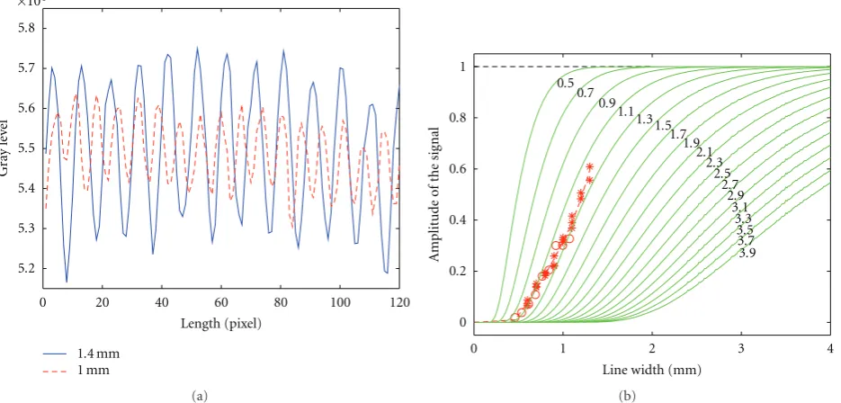
To increase the signal-to-noise ratio, the local contrast of each set of lines of the resolution target is obtained by averaging the realigned pattern (after corrections of residual rotations ensuring perfect horizontality or verticality of the transitions). This average is performed over 50 pixels for the vertical direction and 1,000 pixels for the horizontal one. In Figure 7(a), the change of the gray level is shown for two sizes, namely, 1.4 mm and 1 mm, with a loss of contrast appearing for the smallest marking size.

In Figure 7(b), variations of contrast that would be obtained if the calibration target was seen through a linear optical system of Gaussian transfer function of Full Width at Middle Height (FWMH) ranging from 0.5 to 3.9 mm are plotted in solid lines. These values are given for magnifi-cations of about 20. The experimental curve lies between the lines corresponding to an FWMH of 1.1 and 1.3 mm, meaning that it will be difficult to distinguish correctly elements smaller than these two sizes. Thus, the speckle deposited onto the cylinder must have at least a diameter of 1.2 mm. This characterization is useful for the realistic synthesis of images discussed in Section5.1.

4.2. Lens Distortions. Because of the use of a rotating mirror framing camera and many mirrors between the object and the camera, the estimation of optical distortions is an important step in the experiments. Techniques utilized to determine the distortions of the wholeoptical system require the acquisition of one image per secondary lens. It is different

from procedures followed to analyze quasistatic experiments [17] or even for the case of a dynamic test [18]. Moreover, because of the complexity of the optical chain, it is not possible to project the distortions found onto a polynomial basis as generally performed [6, 17]. In the present case, the frame-to-frame distortions were found negligible with respect to that of the whole optical chain.

The proposed approach to correct for optical distortions consists in resorting to a random numerical texture that is printed onto a plate by laser engraving. The plate and its support are put on a stool. Then, pictures of the plate are shot by the camera. A correlation computation is run between the digital reference and the first image acquired by the camera. This computation, carried out by the technique presented in Section 2.3, provides a displacement field (utot,vtot)

containing all the information concerning magnification, in-and out-of-plane rotation (a first-order approximation can be used in the present case since the distance of the object to the camera is very large), and distortions. To account for these different components, the displacement field is projected onto the following basis

Ua f f =ax+by+c,

Va f f =dx+ey+f . (20)

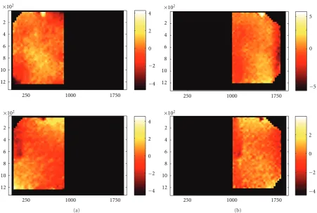
The distortion field corresponds to the displacement residu-als. The type of image obtained in the present case is shown in Figure8(a)for a theoretical image shown in Figure8(b). The junction between the two mirrors gives rise to spurious results. Consequently, the distortions are evaluated indepen-dently for the left and right mirrors (Figures9(a)and9(b)). The amplitudes of the distortions remain small, namely, mean value in the centipixel range, standard deviation in the pixel range, and no particular pattern is caused by the piece of adhesive tape seen in Figure 8(a). Consequently, the influence of optical distortions on the stereoscopic reconstruction of the object is neglected. The fields of distortions are similar for the 25 images of the sequence [19], thereby proving that the frame-to-frame distortions are of secondary influence. Last, no artifacts related to digitization (e.g., discontinuities between successive lines perpendicular to the scan direction) were observed in the analyses performed in the present section. If any, they remain very small in comparison with those induced by the optical chain.

5. Application

0 20 40 60 80 100 120 5.2

5.3 5.4 5_.5 5.6 5.7 5.8

×104

Length (pixel)

Gr

ay

le

ve

l

1.4 mm 1 mm

(a)

0 1 2 3 4

0 1

0.2 0.4 0.6 0.8

Line width (mm)

A

m

plitude

o

f

the

sig

nal

0.5 0_.7

0.9 1.1_1.

3 1.5 1.7

1.9 2.1

2.3 2.5

2.7 2.9

3.1 3.3 3.5 3.7 3.9

(b)

Figure7: (a) Evolution of gray level contrast with the spatial period of the crenels. (b) Normalized contrast versus line width: experimental points (red symbols) and curves (green) obtained for a linear system with a Gaussian transfer function of varying FWMH from 0.5 to 3.9 mm.

(a) (b)

Figure8: Images obtained with stereoscopic mirrors and used for estimating of distortions (a). The white rectangle located on the upper edge of the field corresponds to a piece of adhesive tape used to fix the calibration pattern onto the machine support. Digital images printed on the calibration plate (b). The distorrions of the whole optical chain is assessed by registering the left and right parts of both pictures.

reason why the computation is not carried out with the initial reference but rather with an updated reference that causes a cumulation of measurement errors. A reduction in the size of the reconstructed surface is observed since the points that leave the initial region of interest are not taken into account. To improve the performances of the approach, a precorrection for large displacements is performed. It consists in seeking a uniform translation to apply to the images so that, on average, the region of interest is motionless. Then the DIC algorithm is run using the prior translation as an initialization of the displacement field. This procedure makes the computation faster, more stable and more accurate. Finally, the stereovision technique is applied to the experiment itself [21–24].

5.1. Detection Level. Before applying the stereo-correlation procedure to an experimental case, it is important to evaluate the size and amplitude of defects that can be detected. The hydrodynamic code HESIONE [25] predicts the shape of the specimen at different stages of evolution. For any instant of time, t, the predicted surface is projected onto the actual surface by least squares minimization.

250 1000 1750 2

4

6

8

10

12

×102

−4

−2 0 2 4

250 1000 1750

2

4

6

8

10

12

×102

−4

−2 0 2 4

(a)

250 1000 1750

2

4

6

8

10

12

×102

250 1000 1750

2

4

6

8

10

12

×102

−4

−2

−5

0 0

2 5

(b)

Figure9: Measured distortion taking into account the stereoscopic mirrors, left (a) and right (b) mirrors. The color scale encodes the magnitude of the displacement expressed in pixel (1 pixel=180μm). The top (resp., bottom) figures show the displacement component along the longitudinal (resp., transverse) axis.

some additional perturbations are superimposed to check the resolution of the analysis. They would correspond to localized “bumps” of various diameters (0.5, 1, 5, 10, and 30 mm) and amplitudes (0.125, 0.25, 0.5, 1, 2.5, and 5 mm) as illustrated in Figure10(c). A total of 15 different perturbations are introduced.

Based on the knowledge of the transformation matrix, each point of the 3D surface is projected onto the two image planes to create synthetic left and right stereoscopic image pairs as close as possible to experimental images. When compared with the experimental geometry, the mean distance between the projection into the image of a known 3D point and the corresponding image-point extracted in the image is equal to±5 pixels. The blurring effect of the entire optical chain is taken into account through convolution with a Gaussian filter. 16 image pairs are generated, one of them (reference) containing no perturbation. Two examples of left-right pairs are shown in Figures11(a)–11(d)and11(b)–

11(e). To appreciate the effect of the bumps on the images, the same figure shows the difference between two similar images with and without the perturbations. Figures 11(c)

and11(f)correspond, respectively, to the left and right views. It is to be emphasized that no noise has been added to the images in order to focus on detection issues.

A DIC analysis was performed on those artificial images, based on the same choice of parameters as the one used in

the experiment, namely, 16×16 pixel elements are selected based on the signal-to-noise ratio. A comparison between the measured and prescribed displacements for each bump allows for the evaluation of the resolution. To carry out this analysis, the measured and imposed shapes are unfolded onto a plane as suggested by Luo and Riou [26].

Figure 12(a)shows the prescribed perturbation for the easiest cases (amplitudes of 2.5 mm and 5 mm, left and right, respectively, for a 30 mm diameter bump), while Figure12(b)

is the measured shape. In spite of a large noise affecting the shape of the bump, this perturbation is rather well captured by DIC computations. Figures12(c)and12(d)correspond to smaller perturbations (amplitudes of 125μm and 250μm, left and right respectively, for a 5 mm diameter). Although the perturbations are detected, their sizes and amplitudes cannot be estimated reliably. The reason for this lies in the intrinsic resolution of the DIC analysis performed here with elements of size 16 pixels or 2.9 mm. Thus the entire bump can fit in a two-element wide square. A summary of the results is presented in Figures 13(a) and 13(b) where measured amplitudes and diameter, respectively, normalized by the prescribed counterpart, are shown for all tested cases.

−200

−150

−100

−50

0

50

0 50 100

X(mm)

Y

(mm)

(a)

−200

−150

−100

−50

0

50

0 50 100

X(mm)

Y

(mm)

(b)

−250

−200

−150

−100

−50

−20 0 20 40 60 80

X(mm)

Y

(m

m)

(c)

Figure10: Reference configuration created by mimicking laser marking (a), deformed surface with a known displacement field (b). Addition of local bump defects on the deformed surface (c).

(a) (b) (c)

(d) (e) (f)

Figure11: 3D surface rendering when unfolded onto a plane. Reference (a) and deformed (b) left images, and their difference (c). Reference (d) and deformed (e) right images, and their difference (f).

radius of curvature, and poorly contrasted surface texture), the limit of detection of such bumps is of the order of 5 mm, and a minimum size of about 10 mm is needed to allow for a reliable quantification of the perturbation. Moreover, 250μm amplitudes are resolved reliably for those conditions. These conclusions hold for a fixed element size of 16 pixels.

P

er

imet

er

(mm)

0 50 100

40

60

80

100

120

0 1 2 3 4

Y(mm)

(a)

P

er

imet

er

(mm)

0 50 100

0

20

40

60

80

100 0

1 2 3 4

Y(mm)

(b)

P

er

imet

er

(mm)

0 50 100

40

60

80

100

120

Y(mm)

0 0.05 0.1 0.15 0.2

(c)

P

er

imet

er

(mm)

0 100

0

20

40

60

80

100 0

0.05

Y(mm)

0.1 0.15 0.2

50

(d)

Figure12: Comparison between the imposed (unfolded) surface displacement (left) and as determined from stereoreconstruction from synthetic images (right). The top figures show bumps of 30 mm diameter, and 2.5 mm, or 5 mm amplitudes. The bottom figures show bumps of 5 mm diameter, and 125μm or 250μm amplitudes.

Possible improvements involve drastic changes in the experimental set-up. CCD camera could offer images in digital format directly, thus limiting the digitation step in the analysis. However, access to similar pixel sizes still represents a technical challenge. A better resolution could also be obtained through a higher magnification, at the expense of a smaller frame.

5.2. Large Displacement Handling. In the context of detonics, very high strain levels between consecutive images have to be captured. This fact is a major difficulty for DIC. A specific procedure has been designed to allow for a much more

robust analysis in this context. As a side benefit, displacement fields appear to be less subjected to noise.

0 5 10 15 20 25 30 0

1 2

0.5 1.5 2_.5

Theoretical diameter (mm)

Dimensionless

amplitude

2.5 mm 0.5 mm 0.125 mm

5 mm 1 mm 0.25 mm

(a)

0 5 10 15 20 25 30

Theoretical diameter (mm)

2.5 mm 0.5 mm 0.125 mm

5 mm 1 mm 0.25 mm 0

1 2 3 4 5 6

Dimensionless

d

iamet

er

(b)

Figure 13: Estimated amplitude (normalized by the imposed one) versus diameter for different amplitudes (a). Estimated diameter (normalized by the imposed one) versus diameter for different amplitudes (b).

(a) (b) (c)

Figure14: Illustration of the precorrection: (a) reference image number 13, (b) raw image number 24, (c) corrected image number 24.

by such artifacts. In contrast, a fair prior estimate of the displacement field, which may still be inaccurate, requires DIC to address only the remaining corrections displacements and hence can be tackled with less coarsened images. As this procedure only affects the initial displacement field, it does not affect the final one at convergence as can be checked by perturbing this prior determination, and checking that the final determination is unaffected. This robustness allows for some tolerance on the quality of this first displacement field, and hence, small effects such as the motion of the cylinder axis are neglected.

−50 0 50

0 50

100 150

−50 0 50 100 150

X(mm)

Y (mm)

Z

(mm)

(a)

−50 0 50

0 50

100 150

−50 0

50 100 150

X(mm)

Y (mm)

Z

(mm)

(b)

−100 −50 0 50

100 0

100 200

−50 0 50 100 150

X(mm)

Y_(mm)

Z

(mm)

(c)

Figure15: Reconstruction of the specimen surface at three stages of expansion, image no. 6 (a), image no. 13 (b) and image no. 25 (final one) (c). The deformed mesh represents the reconstruction data while the points represent the interpolated surface.

Section 2once the 3D frames used in the code and in the stereo-correlation procedure coincide. This is achieved by a least squares minimization between the initial experimental and numerical shapes. A mispositioning error of the order of 1 mm is achieved. Figure14illustrates the effect of the prior correction of a late image onto reference one. It can be seen that most of the displacement has been accounted for, and only small differences remain to be determined (by DIC). When this prior determination is not taken into account, a larger element size (24 pixels) has to be chosen to limit the uncertainty level. With the present initialization, a 16 pixel element can be dealt with.

5.3. Experimental Reconstruction. After the experiment, the film composed of 25 acquisitions is developed and the 25 images are digitized independently from each other. From the fixed elements of the scene (yellow paper in Figure1(a)

or the calibration target shown in Figure14), repositioning of images is performed by adjusting a translation correction so that the elements remain motionless [19].

(a) (b)

Figure16: Last image pair (left and right views). On the lower part (inside the red rectangle), a necking appears.

sZ

(mm)

10 15 20 25

0_.2 0.4 0.6 0.8 1.2 1.4 1.6 1.8

1

Image number

(a)

10 15 20 25

0_.2 0_.4 0_.6 0.8 1.2 1.4 1.6 1.8

1

Image number sZ

(mm)

(b)

Figure17: Evolution of surface roughness, evaluated over the entire surface or a central zone, total zone (plain curve), on a central zone (dotted curve) (a) and locally (b).

computed geometries, the two surfaces superimpose quite well for the entire duration of the experiment. Displacement corrections of at most ±20 pixels need to be measured. With the multiscale algorithm used herein, this level is easily measured. Moreover, in the last picture, a clear defect can be identified, which is interpreted as a local thinning of the specimen, that is, an example of necking. The image pair shown in Figure16supports that statement.

In order to investigate on a quantitative basis the onset of necking, it is proposed to base the analysis on the standard deviation of the normal surface displacements. This standard deviation can be seen as a measure of the roughness of the expanding surface, which is expected to remain small for

a uniform strain of the surface, and to display a sudden increase when necking (at least necking that can be captured by the DIC analysis, i.e., at a large enough scale). The standard deviation is expected to be sensitive to the sampled surface as the lower part of the specimen is subjected to a larger strain. Thus the standard deviation is estimated over three regions, namely, first globally over the entire field of analysis, second over a central zone (where edge effects are avoided), and third on a zone located at the bottom of the specimen where necking is seen to occur first.

for the two last stages, although the level of fluctuation of this curve makes this last observation questionable. The central zone shows a smaller roughening, which is consistent with the lower strain level reached in this zone. Let us emphasize the fact that the displacement field is computed from the reference image to the current one, and hence the steady increase cannot be attributed to a cumulation of measurement errors. Note also that the initial image has already a significant roughness because it has suffered a significant expansion prior to be captured in the first image. The third standard deviation computed over the bottom part of the specimen is shown in Figure17(b). The sudden acceleration of the standard deviation for the last images seems to depart clearly from the previous steady evolution and supports the previous discussion on a detectable necking occurring in this zone. This also supports the idea that the global standard deviation is affected by the necking of the lower part, and that the sudden rise is actually meaningful. Moreover, the a priori uncertainty is estimated to amount to 0.5 pixel, or 90μm. The impact of image noise has been estimated to amount to an additional 100μm [19]. The sum of these uncertainties is well below the fluctuation level reported in those graphs.

6. Conclusion

A successful attempt is reported to reconstruct complex 3D displacement fields for high-speed blast experiments under very severe experimental conditions using a rotating mirror high-speed camera. Both large-scale shape changes as well as local features associated with necking can be captured. The techniques were also set up to estimate the resolution and distortions of the optical chain allowing for the analysis of a synthetic case representative of the experimental test.

Specific procedures useful to enhance the performance of such stereo-correlation analyses have been developed. In particular, the combination of precorrections and global digital image correlation algorithm provides both robust and accurate 2D displacement fields that are suitable to stereo-correlation to get three-dimensional displacement fields. Other directions for improving the experiment itself are currently being investigated, namely, surface marking, which can sustain the very strain rates of the specimen, submicrosecond lighting, and digital cameras [27,28] that will in a near future replace the film camera used in the present study. In the same spirit, combining more than two views of the same scene is a stimulating direction for increasing the accuracy of the reconstruction even with images having a low contrast or specular reflections that may always occur unexpectedly [14,29,30]. Stereovision is thus a very powerful tool to analyze high-speed experiments.

Last, let us note that the fact that the observed object is initially cylindrical makes the DIC procedures difficult due to the perspective issues. An a priori knowledge on the initial shape of the object would make the reconstruction step easier and faster. It would also allow to further increase the reconstructed surface area.

References

[1] S. F. Ray,High Speed Photography and Photonics, SPIE, 1997. [2] P. F. Luo, Y. J. Chao, and M. A. Sutton, “Application of stereo

vision to three-dimensional deformation analyses in fracture experiments,”Optical Engineering, vol. 33, no. 3, pp. 981–990, 1994.

[3] P. F. Luo and F. C. Huang, “Application of stereo vision to the study of mixed-mode crack-tip deformations,”Optics and Lasers in Engineering, vol. 33, no. 5, pp. 349–368, 2000. [4] Z. Lei, H.-T. Kang, and G. Reyes, “Full field strain

mea-surement of resistant spot welds using 3D image correlation systems,”Experimental Mechanics, vol. 50, no. 1, pp. 111–116, 2010.

[5] J.-J. Orteu, “3-D computer vision in experimental mechanics,”

Optics and Lasers in Engineering, vol. 47, no. 3-4, pp. 282–291, 2009.

[6] M. A. Sutton, J. J. Orteu, and H. W. Schreier,Image Correlation for Shape, Motion and Deformation Measurements: Basic Concepts, Theory and Applications, Springer, Berlin, Germany, 2009.

[7] F. Barthelat, Z. Wu, B. C. Prorok, and H. D. Espinosa, “Dynamic torsion testing of nanocrystalline coatings using high-speed photography and digital image correlation,” Exper-imental Mechanics, vol. 43, no. 3, pp. 331–340, 2003.

[8] A. Gilat, T. Schmidt, and J. Tyson, “Full field strain mea-surement during a tensile split Hopkinson bar experiment,”

Journal De Physique. IV, vol. 134, pp. 687–692, 2006. [9] V. Tiwari, M. A. Sutton, S. R. McNeill et al., “Application of

3D image correlation for full-field transient plate deformation measurements during blast loading,”International Journal of Impact Engineering, vol. 36, no. 6, pp. 862–874, 2009. [10] P. L. Reu and T. J. Miller, “The application of high-speed digital

image correlation,”Journal of Strain Analysis for Engineering Design, vol. 43, no. 8, pp. 673–688, 2008.

[11] F. Devernay,Vision st´er´eoscopique et propri´et´es diff´erentielles des surfaces, Ph.D. dissertation, Ecole Polytechnique, 1997. [12] L. Duvieubourg, S. Ambellouis, and F. Castestaing,

“Single-camera stereovision setup with orientable optical axes,” in

Proceedings of the International Conference on Computer Vision and Graphics (ICCVG ’04), vol. 32 ofComputational Imaging and Vision, pp. 173–178, Warsaw, Poland, September 2004. [13] H. Zhang and K. Ravi-Chandar, “Nucleation of cracks under

dynamic loading,” in Proceedings of the 12th International Conference on Fracture, 2009.

[14] O. Faugeras,Three-Dimensional Computer Vision: A Geometric Viewpoint, MIT Press, Cambridge, Mass, USA, 1993. [15] M. Devy, V. Garric, and J.-J. Orteu, “Camera calibration

from multiple views of a 2D object, using a global non linear minimization method,” in Proceedings of IEEE/RSJ International Conference on Intelligent Robots and Systems (IROS ’97), Grenoble, France, September 1997.

[16] G. Besnard, F. Hild, and S. Roux, “Finite-element dis-placement fields analysis from digital images: application to Portevin-Le Chatelier bands,”Experimental Mechanics, vol. 46, no. 6, pp. 789–803, 2006.

[17] D. Garcia,Mesure de formes et de champs de d´eplacements tridi-mensionnels par st´er´eo-corr´elation d’images, Ph.D. dissertation, Ecole des Mines d’Albi, 2001.

[18] V. Tiwari, M. A. Sutton, and S. R. McNeill, “Assessment of high speed imaging systems for 2D and 3D deformation measurements: methodology development and validation,”

[19] G. Besnard,Caract´erisation et quantification de surfaces par st´er´eocorr´elation pour des essais m´ecaniques du quasi statique `a la dynamique ultra-rapide, Ph.D. dissertation, Ecole Normale Sup´erieure de Cachan, 2010.

[20] K. Ravi-Chandar, A. B. Albrecht, H. Zhang, and K. M. Liechti, “High strain rate adhesive behavior of polyurea coatings on aluminum,” inProceedings of the 12th International Conference on Fracture, 2009.

[21] G. Besnard, S. Roux, F. Hild, and J. M. Lagrange, “Contactfree characterization of materials used in detonic experiments,” inProceedings of the 34th International Pyrotechnics Seminar Europyro, vol. 2, pp. 815–824, 2007.

[22] G. Besnard, J. M. Lagrange, F. Hild, S. Roux, and C. Voltz, “M´etrologie pour l’exp´erimentation en d´etonique, acc`es au ph´enom`ene de striction,” inNeuvi`eme colloque international francophone du club SFO/CMOI, Nantes, France, 2008. [23] G. Besnard, B. Etchessahar, J. M. Lagrange, C. Voltz, F. Hild,

and S. Roux, “Metrology and detonics: analysis of necking,” inProceedings of the 28th International Congress on High-Speed Imaging and Photonics, pp. 71261N-1–71261N-12, 2008. [24] C. Voltz, J. M. Lagrange, G. Besnard, and B. Etchessahar,

“Application of ultra-high-speed optical observations and high-speed Xray radiography measurements to the study of explosively driven copper tube expansion,” inProceedings of the 28th International Congress on High-Speed Imaging and Photonics, pp. 71261M–71261M10, 2008.

[25] “HESIONE: CEA-DAM 3D Hydrodynamic code”.

[26] P. F. Luo and S. S. Liou, “Measurement of curved surface by stereo vision and error analysis,” Optics and Lasers in Engineering, vol. 30, no. 6, pp. 471–486, 1998.

[27] http://www.shimadzu.com/products/test/hsvc/index.html.

[28] http://www.cordin.com/products.html.

[29] N. Ayache and F. Lustman, “Trinocular sterovision for robotics,” INRIA report 1086, INRIA, 1989.