Time dependence of Poisson’s effect in wood IV: influence of grain angle

(1)

O R I G I N A L A R T I C L E

Time dependence of Poisson’s effect in wood IV: influence of grain

angle

Ken Kawahara1•_{Kosei Ando}1•_{Yusuke Taniguchi}2

Received: 19 January 2015 / Accepted: 24 March 2015 / Published online: 12 April 2015

ÓThe Japan Wood Research Society 2015

Abstract Off-axis tensile creep tests were conducted on

woods taken from Japanese cypress and Kalopanax by changing the angle of load to the grain direction in the longitudinal–tangential (LT) plane. The dependence of the Poisson’s ratio and trend of the viscoelastic Poisson’s ratio on grain angle were investigated. The Poisson’s ratios were found to reach their extrema when the grain angle was around 30°. Moreover, the Poisson’s ratio in the LT plane was observed to be negative when the grain angle was in the range of 15°–45°. Comparing the experimental results with theoretical values obtained from the theory of orthotropic elasticity, it was revealed that, although the Poisson’s ratio reached an extremum in both cases, the specific values did not match, especially when the angle was between 15°and 45°. Furthermore, the temporal var-iation of the viscoelastic Poisson’s ratio was found to de-pend on the grain angle and the measurement plane. It also appeared to be affected by the Poisson’s ratio, showing an increasing tendency above a specific Poisson’s ratio (Ja-panese cypress: 0.196, Kalopanax: 0.102) and a decreasing tendency below it, regardless of the grain angle and mea-surement plane. Additionally, the increment in the vis-coelastic Poisson’s ratio after 24 h of creep was observed to reach its extremum when the grain angle was around 30°. Finally, by improving the six-element Frandsen– Muszynski viscoelastic model, which simultaneously con-siders the longitudinal and transverse strains, an

eight-element model was presented, and the trend of the vis-coelastic Poisson’s ratio was well reproduced by this model.

Keywords Poisson ratioGrain angleShear effect

Viscoelasticity Creep

Introduction

Wood is a material that has been used for building structures since ancient times. Despite the importance of studying its mechanical behavior, many aspects are still poorly under-stood. One of the main characteristics of the mechanical behavior of wood is anisotropy; wood is known to be an orthotropic material, and its strength varies significantly with cellular orientation and arrangement. The strength in the longitudinal (L) direction of the grain is dominantly high, followed by that in the radial (R) direction, and then by that in the tangential (T) direction. Although there have been many studies on anisotropy in directions other than the three principal axes (axes of symmetry), almost all of them con-sider only the Young’s modulus, shear modulus, and strength. For instance, Hearmon [1] investigated the varia-tion in Young’s modulus and shear modulus with respect to the grain angle in spruce. Kollmann [2] determined the elements of the elastic compliance matrix, i.e., Young’s moduli and shear moduli in the three principal stress di-rections, for 17 wood species. Moreover, he used Hankin-son’s equation [3] to study the variation in tensile strength with grain angle for white fir and basswood.

In comparison, there have been relatively few researches into the anisotropy of the Poisson’s ratio of wood [4–17]. The Poisson’s ratios in the direction of the principal axes of wood are defined as follows:

& Kosei Ando

[email protected]

1 _{Graduate School of Bioagricultural Sciences, Nagoya}

University, Chikusa-ku, Nagoya 464-8601, Japan

2 _{Building Products Headquarters, Daiken Corporation,}

(2)

mij¼

ej

ei

i;j¼ L; T; R

ð Þ; ð1Þ

where ei is the longitudinal strain, ej is the transverse strain, and the subscripts i and j denote the directions along the three principal axes. Because of the lack of definite relationships between the Poisson’s ratios and other elastic constants, density, or strength [18] and our limited understanding of how Poisson’s ratio varies in different directions, many aspects of the formation mechanism of Poisson’s ratio in wood remain unclear. Similar to the Young’s modulus and shear modulus, the Poisson’s ratio is an independent elastic constant that has significant influence on the stress–strain relationship of a material, especially under combined stresses. With in-creasingly complex and diversified structures being de-veloped using wood, it is important to elucidate the formation mechanism for the anisotropy of its Poisson’s effect, on which several studies have been conducted. Yamai [4] derived the Poisson’s ratios for nine wood species in the directions along the grain and perpendicular to the grain through compression tests, and he found that the Poisson’s ratio is not related to the specific gravity. Moreover, he theoretically investigated the dependence of Poisson’s ratio on grain angle by applying the theory of orthotropic elasticity to experimental data and showed that the Poisson’s ratio may be negative at some incli-nation angles. Although the Poisson’s ratio of isotropic materials is generally positive, it has been pointed out that porous materials can have negative Poisson’s ratios [19]. Sliker et al. [7] investigated the dependence of the Pois-son’s ratios in the LT and LR planes on grain angle in 18 hardwood species through tensile tests. They reported that the rate of change of Poisson’s ratio with the angle of load to the L direction was greater in the LT plane than in the LR plane. In the LT plane, the Poisson’s ratios of some wood species were negative at 20°grain angle (this supports the theory of orthotropic elasticity), and the grain angle corresponding to the minimum value differed by species. On the other hand, in the LR plane, all the wood species had non-negative Poisson’s ratios regardless of the grain angle. Bukur et al. [20] and Murata et al. [13] also recorded negative Poisson’s ratios in experimental data of woods. Since then, research into the dependence of the Poisson’s ratio of wood on the grain angle, annual-ring angle, or microfibril angle has included several ex-perimental and theoretical studies, which have reported extreme values at inclination angles of 20°–45° [8–13]. However, there has also been a report of a different tendency observed in the Poisson’s ratio of a tropical wood, which decreases with increasing grain angle with-out reaching an extremum [14]. It could not be explained why this tendency differs.

In addition to anisotropy, another important characteristic of the mechanical behavior of wood is its viscoelastic property. Therefore, to grasp the mechanical response of wood under long-term loading, the time dependence of Poisson’s effect must be analyzed. As Poisson’s ratio is an elastic constant, it does not change with time; the parameter that characterizes the time-dependent Poisson’s effect is called the viscoelastic Poisson’s ratio. There have been several studies on the viscoelastic Poisson’s ratio of wood in the directions of the principal axes [21–30]. Taniguchi et al. [27] conducted tensile creep tests on 12 wood species to measure mLR(t) and mLT(t) and experimentally verified that

both increase with timet. As in the case of the longitudinal strain, the transverse strain during creep can be decomposed into three components, namely instantaneous strain, delayed elastic strain, and permanent strain. Taniguchi et al. also verified that the main cause for the increase in viscoelastic Poisson’s ratio during creep is the considerable increase in the permanent transverse strain. Moreover, Taniguchi et al. [26] and Ando et al. [29] conducted tensile creep tests on Japanese cypress in the direction of the three principal axes and measured the transition of the six viscoelastic Poisson’s ratios [mLR(t),mLT(t),mRL(t),mRT(t),mTL(t), andmTR(t)]. Their

results revealed that all the viscoelastic Poisson’s ratios in-crease logarithmically with creep time and that the vis-coelastic compliance matrix is non-symmetric, unlike the symmetric elastic compliance matrix. Ozyhar et al. [30] performed tensile and compressive creep tests on beech wood and reported that the six viscoelastic Poisson’s ratios increased in tension and decreased in compression and that the viscoelastic compliance matrix was non-symmetric, confirming the results of Ando et al.

When wood is used as a building material, loads can be generated in various directions with respect to the grain, not necessarily in the directions of the principal axes. Therefore, the shear forces arising in the direction of the principal axes are significant, and it is important to un-derstand the behavior of the viscoelastic Poisson’s ratio under the shearing effect. However, there has been almost no research into the variation of the viscoelastic Poisson’s ratio with respect to the grain angle of wood.

In this study, 24 h off-axis tensile creep tests were conducted on the LT plane of two wood species, Japanese cypress and Kalopanax, and the dependence of the Pois-son’s effect on grain angle and creep time was investigated.

Materials and methods

Materials

(3)

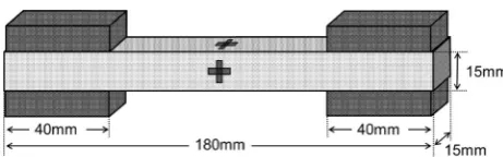
(Kalopanax septemlobus Koidz.) woods were chosen as test samples in this study. The specimens for the tensile creep tests were cut from a sawn board, and, by changing the loading direction in the LT plane from the L direction to the T direction, specimens of seven different grain an-gles were prepared (0°, 15°, 30°, 45°, 60°, 75°, and 90°), as illustrated in Fig.1. The angles 0°and 90°correspond to the L direction and T direction, respectively, and the R direction is always perpendicular to the direction of load-ing. The dimensions of the specimens were 1809159 15 mm (Fig.2), and the grip sections of length 40 mm on both ends of the specimen were reinforced by tabs made of a hardwood.

All the specimens were conditioned to equilibrate a moisture content at a constant 25°C and 55 % relative humidity (RH). The densities of these air-dried Japanese cypress and Kalopanax specimens were 417±7 and 545±7 kg/m3, respectively; their moisture contents were 9.4±0.6 and 9.6±0.1 %, respectively, and the widths of their annual rings were 0.84 and 1.92 mm, respectively.

Off-axis tensile creep tests

The off-axis tensile tests were performed using a universal testing machine (Shimadzu Autograph AGX-100kN). Bi-axial strain gauges (gauge length: 2 mm; Tokyo Sokki Kenkyujo, FCA-2-11) were attached to the central regions of the four planes of the specimen to measure both the longitudinal and transverse strains, which were reported as the average of the values from the corresponding opposite planes. The viscoelastic Poisson’s ratio on the LT plane of

the specimen is denoted asmLT(a,t) (Fig.1), whereais the

grain angle (°), andtis the creep time (h). The viscoelastic Poisson’s ratio on the plane perpendicular to the LT plane, i.e., the plane whose normal direction changes from the T to L with increasing grain angle, is denoted as mLR(a, t)

(Fig.1). Therefore, as the grain angle increases from 0°to 90°, the corresponding Poisson’s ratios change frommLTto

mTLand frommLRtomTR.

The tensile creep tests were conducted for 24 h. Although a 24-h period from the start is considered an early stage of creep in wood, permanent strains are generated during this period, and therefore it was assumed that the creep behaviors in this study are similar to those from long-period tests. The applied stress was 40 % of the tensile strength, which was determined in advance from static tensile tests (Table1), and the target load was reached in 10 s. At least five samples were prepared for each grain angle, but the number of samples varied depending on the cutting procedure from one board. During the tests, the temperature and humidity were maintained at 25°C and 55 % RH, respectively.

ν_LR(0,t)

ν_LT(0,t)

ν_LR(15,t)

ν_LT(15,t)

ν_LR(30,t)

ν_LT(30,t)

ν_LR(45,t)

ν_LT(45,t)

ν_LR(60,t)

ν_LT(60,t) ν_LT(75,t)

ν_LR(75,t) ν LR(90,t)

ν_LT(90,t)

0° 15°

75° 60°

45° 30°

90°

L

T R

Fig. 1 Schematic of off-axis tensile specimens.mLT(a,t) andmLR(a,t) represent the viscoelastic Poisson’s ratios.agrain angle (°),tcreep time

(h)

Fig. 2 Tensile test specimen. A biaxial strain gauge was attached on

(4)

Results and discussion

Young’s modulus

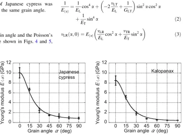
The Young’s moduli of Japanese cypress and Kalopanax obtained from the experiments at the various grain angles are presented in Fig.3, in which the solid line represents the theoretical values calculated in accordance with Eq. (2) described later in this section. For both the wood species, the Young’s modulus dropped rapidly as the grain angle first increased from 0°and then decreased gradually with further increase in the grain angle. At 0° grain angle, the Young’s modulus of Japanese cypress was 10.0 GPa, and that of Kalopanax was 8.5 GPa. At 90° grain angle, the Young’s modulus of Japanese cypress was 0.9 GPa, and that of Kalopanax decreased to 0.5 GPa. In the entire range, the Young’s modulus of Japanese cypress was higher than that of Kalopanax at the same grain angle.

Poisson’s ratio

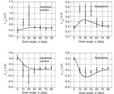
The relationships between the grain angle and the Poisson’s ratiosmLR(a, 0) and mLT(a, 0) are shown in Figs.4 and 5,

respectively, for both the Japanese cypress and Kalopanax. The Poisson’s ratio was taken at creep timet =0, i.e., at the start of the test, and the solid lines represent the theoretical values obtained from Eqs. (3) and (4), which are described later in this section. On both planes, the Poisson’s ratio reached an extremum around a grain angle of 30°. However, the manner in which the extremum was approached differed: mLR(a, 0) was convex upward, whereasmLT(a, 0) was convex

downward. Furthermore,mLT(a, 0) exhibited the same

ten-dency as the experimental results published by Sliker et al. [7], who conducted off-axis tensile tests in the LT plane on specimens of 18 hardwood species. According to their re-sults, mLT(a, 0) convexed downward and reached the

ex-tremum at a grain angle of 20°; whereas, in our study, it varied greatly at same grain angle within the range 15°–45°. Because of significant shearing effect along the L direction and its variation due to the inhomogeneity and mounting conditions of the tensile wood specimen, it was difficult to accurately measure the Poisson’s ratio at these grain angles. Moreover, the Poisson’s ratiosmLT(a, 0) of some specimens

were negative in the range 15°–60°, implying that the spe-cimen extended in the transverse direction when the tensile load was applied. This phenomenon, which is unlikely in isotropic materials, was assumed to occur because of the large shearing effect along the L direction and was investi-gated using the following theoretical equations that include this shearing effect.

Applying the generalized Hook’s law to the orthotropic specimen with grain angle a, the following equations are obtained [31,32]:

1 EðaÞ

¼ 1 EL

cos4aþ 2mLT EL

þ 1 GLT

sin2acos2a

þ 1 ET

sin4a ð2Þ

mLRða;0Þ ¼EðaÞ

mLR EL

cos2aþmTR ET

sin2a

ð3Þ

Japanese cypress

Kalopanax

0 2 4 6 8 10 12

0 15 30 45 60 75 90

Yo

u

n

g'

s

mo

d

u

lu

s

E

㻔

䃐

㻕㻌

(G

Pa

)

Grain angle 䃐(deg)

0 15 30 45 60 75 90

0 2 4 6 8 10 12

Y

o

un

g

's

m

o

du

lu

s

E

㻔

䃐

㻕㻌

(G

Pa

)

Grain angle 䃐 (deg)

Fig. 3 Young’s modulusE(a)as

a function of the grain angle. Thesolid linerepresents a fit according to the theory of orthotropic elasticity used to estimate the shear modulusGLT (Eq.2).Error barstandard deviation

Table 1 Creep stresses and number of specimens at different grain

angles

Angle (°) Japanese cypress Kalopanax

n Creep stress (MPa)

0 9 44.0 13 35.4

15 6 17.8 7 22.0

30 9 6.4 7 10.1

45 5 3.4 7 5.7

60 8 2.3 5 3.9

75 7 1.8 7 3.2

90 7 1.7 6 3.0

(5)

mLTða;0Þ ¼ EðaÞ

1 EL

þ 1 ET

sin2acos2a

mLT EL

ðcos4_a_þ_sin4_a_Þ 1 GLT

sin2acos2a

ð4Þ

in whichE(a)is the Young’s modulus in the direction along

the grain angle a, EL is the Young’s modulus in the L

direction, ET is the Young’s modulus in the T direction,

andGLT is the shear modulus in the LT plane. The

theo-retical values of the Poisson’s ratiosmLR(a, 0) andmLT(a, 0)

were calculated from Eqs. (3) and (4), respectively, using the elastic parameters tabulated in Table2. The values of EL, ET, mLT, mLR, and mTR used were taken from

ex-perimental measurements. Moreover,GLTwas obtained by

using Eq. (2) and applying the least-squares regression method so that the sum of the squared differences was minimized between the experimental measurements ofE(a)

for different grain angles and the corresponding values of E(a) calculated using the estimated GLT (and the

experimental values of EL, ET, and mLT). The regression

results are shown in Fig.3as a solid line, and it can be seen that they roughly match with the experimental measure-ments. The estimated GLT was 0.804 GPa for Japanese

cypress and 0.644 GPa for Kalopanax.

The theoretical values of the Poisson’s ratiosmLR(a, 0)

andmLT(a, 0) at various grain angles are presented as solid

lines in Figs.4and5, respectively. At grain angles between 15°and 75°for Kalopanax, negative values were obtained formLT(a, 0), implying that a shearing effect occurs in the L

direction. On the other hand, the theoretical mLT(a, 0) for

Japanese cypress did not show negative values even though some of the corresponding experimental values were negative. This difference between the two wood species is most likely due to the sensitivity of the analytical values from Eq. (4) to the estimated GLTvalues. For both wood

species,mLR(a, 0) was convex upward,mLT(a, 0) was

con-vex downward, and the measured and theoretical results were consistent in the manner of the Poisson’s ratios reaching their respective extrema. However, the values

Kalopanax Japanese

cypress

0.2 0.4 0.6 0.8 1.0 1.2 1.4

0 15 30 45 60 75 90

䃜

LR

㻔

䃐

,0

㻕

0.2 0.3 0.4 0.5 0.6 0.7 0.8 0.9

0 15 30 45 60 75 90

䃜

LR

㻔

䃐

,0

㻕

Fig. 4 Poisson’s ratiomLR(a, 0)

as a function of the grain angle. Thesolid linerepresents a fit according to the theory of orthotropic elasticity (Eq.3). Error barstandard deviation

Japanese cypress

Kalopanax

-0.6 -0.4 -0.2 0.0 0.2 0.4 0.6

0 15 30 45 60 75 90

䃜

LT

㻔

䃐

,0

㻕

-0.6 -0.4 -0.2 0.0 0.2 0.4 0.6

0 15 30 45 60 75 90

䃜

LT

㻔

䃐

,0

㻕

Fig. 5 Poisson’s ratiomLT(a, 0)

as a function of the grain angle. Thesolid linerepresents a fit according to the theory of orthotropic elasticity (Eq.4). Error barstandard deviation

Table 2 Elastic parameters

used in the calculations of Eqs. (2), (3), and (4)

Species EL(GPa) mLT mLR mTR ET(GPa) GLT(GPa)

Japanese cypress 10.05 0.432 0.408 0.491 0.877 0.804

(6)

itself were not well matched, especially between 15° and 45°. Two reasons were considered to explain the noticeable discrepancies between the measured and theoretical results, especially at grain angles in the range of 15°–45°. The first reason is that Eqs. (3) and (4), which were used to calculate the theoretical values, are two-dimensional (2D) equations, and therefore cannot fully express the three-dimensional phenomena, i.e., the effects from the vertical plane. The second reason is that variations in the influence of the shear forces on the L direction arise because of the inhomo-geneity and mounting conditions of the wood specimens, especially at grain angles in the range of 15°–45°.

Viscoelastic Poisson’s ratio

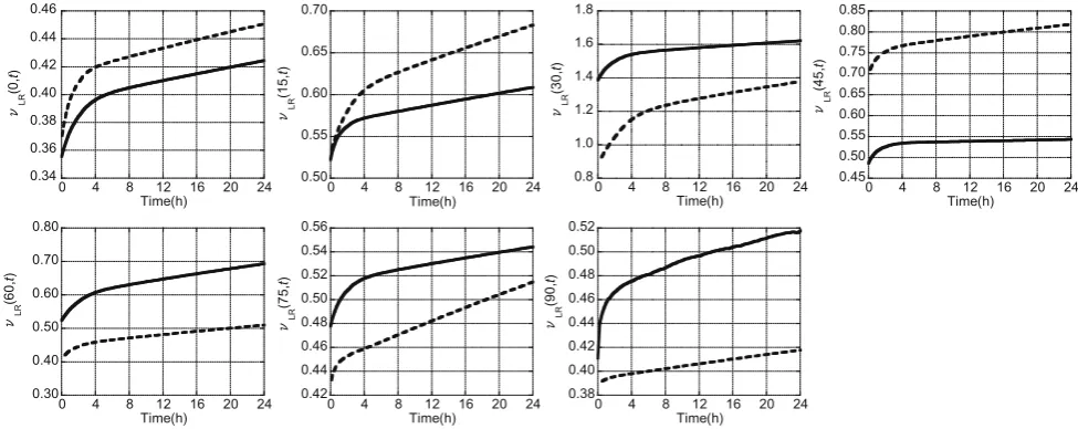
Typical cases of the evolution of the viscoelastic Pois-son’s ratiosmLR(a,t) andmLT(a,t), obtained from the 24 h

creep tests on Japanese cypress and Kalopanax specimens, are plotted for the various grain angles in Figs.6 and7, respectively. In these figures, the solid lines represent Japanese cypress, and the dotted lines represent Kalopa-nax. In all cases, the viscoelastic Poisson’s ratios first underwent rapid change once creep started, and then showed more gradual change over time. For both wood species,mLR(a,t) increased regardless of the grain angle;

whereas mLT(a, t) increased at the grain angle of 0°,

in-creased or dein-creased at the grain angle of 15°, and de-creased at the grain angles equal to or greater than 30°. However, the results shown in Figs.6and7are only from one set of specimens, and thus it cannot be concluded that all specimens at a certain grain angle will show the same trend. For example, although themLT(15, t) of the

Kalo-panax specimen presented in Fig.7increased, there were specimens that showed a decrease in the mLT(15, t).

Therefore, to express the creep test results quantitatively with respect to grain angle, the increments in the vis-coelastic Poisson’s ratios after 24 h of creep will be ex-amined next.

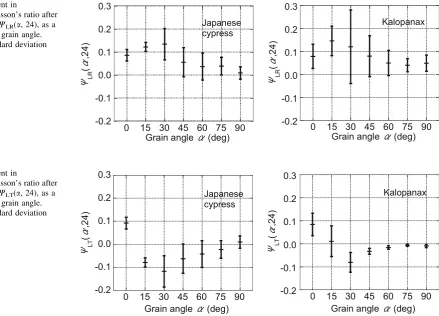
The increment in the viscoelastic Poisson’s ratio with creep time t(h) is defined by the following equation: WLiða;tÞ ¼mLiða;tÞ mLiða;0Þ ði¼ R, TÞ ð5Þ

The increments in the viscoelastic Poisson’s ratios after 24 h of creep, WLR(a, 24) and WLT(a, 24), are

plotted against the grain angle in Figs.8 and 9, respec-tively. Both quantities approached the extrema around a grain angle of 30° in the two wood species, but WLR(a,

24) was convex upward; whereasWLT(a, 24) was convex

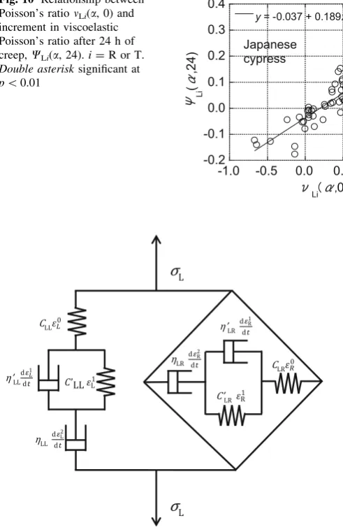
downward. These trends are similar to the dependence of the Poisson’s ratios on grain angle previously shown in Figs.4 and 5. Without taking into account the grain angle and measurement plane, the relationship between the Poisson’s ratio and the increment in the viscoelastic Poisson’s ratio att=24 h is presented in Fig.10for the two wood species. According to the results of linear regression, these two parameters are positively correlated with a 1 % significance level. The regression results also suggested that there exists a Poisson’s ratio (denoted as m0) at zero increment of viscoelastic Poisson’s ratio.

From the regression equation, the values of this Pois-son’s ratio were obtained as m0=0.196 for Japanese

cypress andm0=0.102 for Kalopanax. Regardless of the

grain angle and measurement plane, the viscoelastic Poisson’s ratio showed an increasing tendency at Pois-son’s ratios above m0 and a decreasing tendency at

Poisson’s ratios below m0, i.e., the influence of the

Poisson’s ratio on the trend of the viscoelastic Poisson’s ratio was evident.

0.34 0.36 0.38 0.40 0.42 0.44 0.46

0 4 8 12 16 20 24

䃜LR

(0

,

t

)

Time(h)

0.50 0.55 0.60 0.65 0.70

0 4 8 12 16 20 24

䃜LR

(15

,

t

)

Time(h)

0.45 0.50 0.55 0.60 0.65 0.70 0.75 0.80 0.85

0 4 8 12 16 20 24

䃜LR

(45

,

t

)

Time(h)

0.30 0.40 0.50 0.60 0.70 0.80

0 4 8 12 16 20 24

䃜LR

(6

0,

t

)

Time(h)

0.42 0.44 0.46 0.48 0.50 0.52 0.54 0.56

0 4 8 12 16 20 24

䃜

LR

(75

,

t

)

Time(h)

0.38 0.40 0.42 0.44 0.46 0.48 0.50 0.52

0 4 8 12 16 20 24

䃜LR

(90

,

t

)

Time(h) 0.8

1.0 1.2 1.4 1.6 1.8

0 4 8 12 16 20 24

䃜LR

(30

,

t

)

Time(h)

(7)

Estimation of viscoelastic Poisson’s ratio using a 2D viscoelasticity model

To express the 2D viscoelasticity of wood, Frandsen et al. [25] proposed a six-element model (Frandsen–Muszynski model) that included the components of instantaneous

strain and delayed elastic strain in both the longitudinal and transverse directions. In this study, their model was im-proved by adding the permanent strain components, and thus an eight-element 2D creep model was obtained, as illustrated in Fig. 11 (longitudinal strain direction: L, transverse strain direction: R). It can be confirmed 0.35

0.40 0.45 0.50 0.55

0 4 8 12 16 20 24

䃜LT

(0,

t

)

Time(h)

-0.3 -0.2 -0.1 0.0 0.1 0.2 0.3

0 4 8 12 16 20 24

䃜

LT

(15,

t

)

Time(h)

-0.30 -0.25 -0.20 -0.15 -0.10 -0.05

0 4 8 12 16 20 24

䃜

LT

(30,

t

)

Time(h)

-0.14 -0.12 -0.10 -0.08 -0.06 -0.04 -0.02

0 4 8 12 16 20 24

䃜

LT

(45,

t

)

Time(h)

-0.10 -0.05 0.00 0.05 0.10 0.15

0 4 8 12 16 20 24

䃜

/7

(60,

t

)

Time(h)

0.02 0.03 0.04 0.05 0.06 0.07

0 4 8 12 16 20 24

䃜

㻸㼀

(75,

t

)

Time(h)

0.02 0.03 0.04 0.05 0.06 0.07 0.08 0.09

0 4 8 12 16 20 24

䃜

㻸㼀

(90,

t

)

Time(h)

Fig. 7 Typical progression of viscoelastic Poisson’s ratiomLT(a,t) measured during creep.Solid lineJapanese cypress,dotted lineKalopanax

Japanese cypress

Kalopanax

-0.2 -0.1 0.0 0.1 0.2 0.3

0 15 30 45 60 75 90

䃇

LR

(

䃐

,2

4

)

-0.2 -0.1 0.0 0.1 0.2 0.3

0 15 30 45 60 75 90

䃇

LR

(

䃐

,2

4

)

Fig. 8 Increment in

viscoelastic Poisson’s ratio after 24 h of creep,WLR(a, 24), as a function of the grain angle. Error barstandard deviation

Japanese cypress

Kalopanax

-0.2 -0.1 0.0 0.1 0.2 0.3

0 15 30 45 60 75 90

䃇

LT

(

䃐

,2

4

)

-0.2 -0.1 0.0 0.1 0.2 0.3

0 15 30 45 60 75 90

䃇

LT

(

䃐

,2

4

)

Fig. 9 Increment in

(8)

experimentally that the transverse strain in wood under-going creep also consists of instantaneous strain, delayed elastic strain, and permanent strain [27], similar to the longitudinal strain. Therefore, the proposed model that considers these three strain components is appropriate. In Fig.11, the section on the left represents the longitudinal strain, and the section on the right represents the transverse strain resulting from Poisson’s effect. Each of them is represented by a series arrangement of a spring, Kelvin– Voigt element, and dashpot.CandC0 denote the stiffness moduli of the springs;g andg0 denote the viscosity coef-ficients of the dashpots. The total longitudinal strain in the L direction,eL, is expressed as the sum of the instantaneous strain in the spring, e0

L, the delayed elastic strain in the Kelvin–Voigt element,e1

L, and the permanent strain in the dashpot,e2

L, yielding the following equation:

eL¼e0_Lþe1_Lþe2_L ð6Þ

Similarly, the total transverse strain in the R direction, eR, can be defined as the sum of the instantaneous straine0

R, the delayed elastic strain e1

R, and the permanent strain e 2 R, yielding the following equation:

eR¼e0Rþe 1 Rþe

2

R ð7Þ

For the instantaneous strain, delayed elastic strain, and permanent strain components, the relationship between the stress in the L direction,rL, and the respective strain can be

written as follows (Fig.11): rL ¼CLLe0LþCLRe

0

R ð8Þ

rL ¼C_LL0 e1_Lþg0_LLde 1 L dt þC

0

LRe 1 Rþg

0

LR de1

R

dt ð9Þ

rL ¼gLL de2

L dt þgLR

de2 R

dt ð10Þ

The stress in the R direction, rR, can be expressed in a

similar manner. For each of the three strain components (i– iii), matrix notation can be used to obtain the following:

(i) instantaneous strain rL

rR

¼ CLL CLR CRL CRR

e0 L e0 R

ð11Þ

or e0

L e0 R

¼ C_CLL CLR RL CRR

1 rL rR

ð12Þ

(ii) delayed elastic strain

rL rR

¼ C

0

LL C

0

LR C_RL0 C_RR0

e1 L e1 R

þ g

0

LL g

0

LR g0RL g0RR

de1 L dt de1

R dt

0 B @

1 C A

ð13Þ

Rearranging gives:

Japanese cypress

Kalopanax

-0.2 -0.1 0.0 0.1 0.2 0.3 0.4

-1.0 -0.5 0.0 0.5 1.0 1.5

y = -0.037 + 0.189x R= 0.862䠆䠆

䃇

Li

(

䃐

,24)

䃜_Li㻔䃐㻘0㻕

-0.2 -0.1 0.0 0.1 0.2 0.3 0.4

-0.5 0.0 0.5 1.0

y = -0.020 + 0.199x R= 0.745䠆䠆

䃇

Li

(

䃐

,24

)

䃜_Li㻔䃐㻘0㻕

Fig. 10 Relationship between

Poisson’s ratiomLi(a, 0) and

increment in viscoelastic Poisson’s ratio after 24 h of creep,WLi(a, 24).i=R or T.

Double asterisksignificant at p\0.01

Fig. 11 2D viscoelastic model considering Poisson’s effect (modified

(9)

de1 L dt de1 R dt

0 B @

1 C A¼ g

0

LL g0LR g0

RL g0RR

1 rL rR

g

0

LL g0LR g0

RL g0RR

1

C0_LL C0_LR C_RL0 C0_RR

e1 L e1 R

ð14Þ

In uniaxial creep tests, rR=0. After simple

replace-ment, the equation above can be summarized as follows: g0LL g0LR

g0RL g0RR

1

¼ a b

c d

ð15Þ

g0_LL g0_LR g0RL g0RR

1

C0_LL C0_LR C0_RL C0_RR

¼ e f

g h

ð16Þ

de1 L

dt ¼arL ee 1 Lþfe

1 R

ð17Þ

de1 R

dt ¼crL ðge 1 Lþhe

1

RÞ ð18Þ

Equation (17) can be re-arranged into as

e1_R¼ 1 f

de1 L

dt

e fe

1 Lþ

a

f rL ð19Þ

Differentiating Eq. (19) with respect to timetyields de1

R dt ¼

1 f

d2e1 L dt2

e f

de1 L

dt ð20Þ

Substituting Eqs. (19) and (20) into Eq. (18) and rearranging,

d2e1 L dt2 þ

de1 L

dt ðeþhÞ þe 1

LðehfgÞ ¼rLðahfcÞ ð21Þ

After simple replacement, Eq. (21) becomes

eþh¼2p;ehfg¼q;rLðahfcÞ ¼r ð22Þ d2e1

L dt2 þ

de1 L dt 2pþe

1

Lq¼r ð23Þ

Solving the differential Eq. (23) with the initial condi-tion e1

L ¼0 at t=0 gives

e1L¼C1ek1t1þC2ek2t1; ð24Þ where

C1¼

r ppffiffiffiffiffiffiffiffiffiffiffiffiffip2_q_þ_aq_r

L

2qpffiffiffiffiffiffiffiffiffiffiffiffiffip2_q ð25Þ

C2¼ r q

r ppffiffiffiffiffiffiffiffiffiffiffiffiffip2_q_þ_aq_r

L

2qpffiffiffiffiffiffiffiffiffiffiffiffiffip2_q ð26Þ k1¼pffiffiffiffiffiffiffiffiffiffiffiffiffip2_q_p; _k2_¼pffiffiffiffiffiffiffiffiffiffiffiffiffi_p2_q_p _ð27Þ

Similarly, the transverse strain component e1

R can be computed by the following equation:

e1_R¼C3 ek3t1

þC4 ek4t1

ð28Þ

4000 4100 4200 4300 4400 4500 4600 4700

0 4 8 12 16 20 24 Experimental Theoretical

䃔

L

(

t

) (

㽢

10

-6 )

Time(h)

-2500 -2000 -1500 -1000

䃔

R

(

t

)

䢪䤸

䢳䢲

䢯䢸䢫

Time(h)

-2500 -2000 -1500 -1000

䃔

T

(

t

)

䢪䤸

䢳䢲

䢯䢸䢫

Time(h)

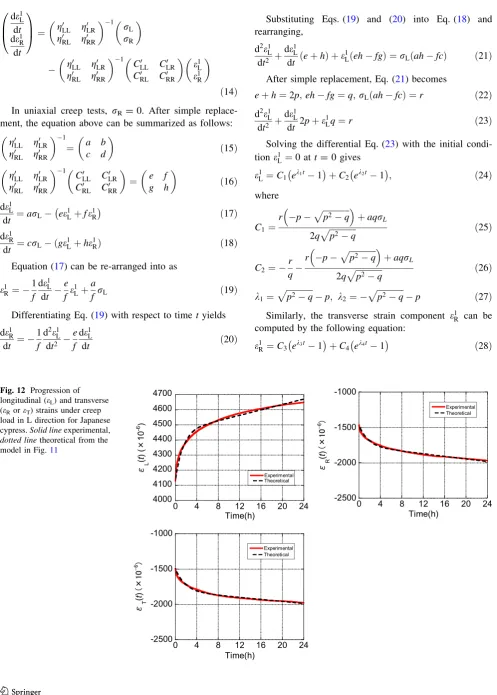
Fig. 12 Progression of

(10)

(iii) permanent strain

rL rR

¼ gLL gLR gRL gRR

de2L dt de2

R dt 0 B @ 1 C A ð29Þ or de2

L dt de2 R dt 0 B @ 1 C

A¼ gLL gLR g_RL g_RR

1 rL rR

ð30Þ

Integrating Eq. (30) with respect to timetwith the initial conditionse2

L¼0 ande 2

R¼0 at t=0 yields

e2 L e2 R

¼ gLL gLR gRL gRR

1 rL rR

t ð31Þ

As can be seen, the permanent strains e2 L and e

2 R are proportional to timet. The constants of proportionality are defined asAandB, respectively.

Thus, from (ii) and (iii), the longitudinal and transverse creep strains can be expressed as follows:

e1_Lþe2_L¼C1 ek1t1

þC2 ek2t1

þAt ð32Þ

e1 Rþe

2

R¼C3 ek3t1

þC4 ek4t1

þBt; ð33Þ

where C1, C2, C3, C4, k1, k2, k3, k4, A, and B are the

constants from the stiffness moduli of the springs, viscosity 0.35 0.36 0.37 0.38 0.39 0.40 0.41 0.42 0.43

0 4 8 12 16 20 24

Experimental 䃜LR Theoretical 䃜LR Experimental㻌䃜LT Theoretical 䃜LT

䃜Li (0 , t ) Time(h) 0.1 0.2 0.3 0.4 0.5 0.6 0.7

0 4 8 12 16 20 24

Experimental 䃜LR Theoretical 䃜LR Experimental 䃜LT Theoretical 䃜LT

䃜 Li (1 5 , t ) Time(h) -1.0 -0.5 0.0 0.5 1.0 1.5 2.0

0 4 8 12 16 20 24

䃜 Li (30, t ) Time(h) -0.2 0.0 0.2 0.4 0.6 0.8

0 4 8 12 16 20 24

Experimental 䃜LR Theoretical 䃜LR Experimental 䃜LT Theoretical㻌䃜LT

䃜 Li (45 , t ) Time(h) 0.0 0.1 0.2 0.3 0.4 0.5 0.6 0.7

0 4 8 12 16 20 24

䃜 Li (6 0 , t ) Time(h) 0.0 0.1 0.2 0.3 0.4 0.5 0.6

0 4 8 12 16 20 24

䃜Li (7 5 , t ) Time(h) 0.0 0.1 0.2 0.3 0.4 0.5 0.6 0.7

0 4 8 12 16 20 24

䃜 Li (90 , t ) Time(h)

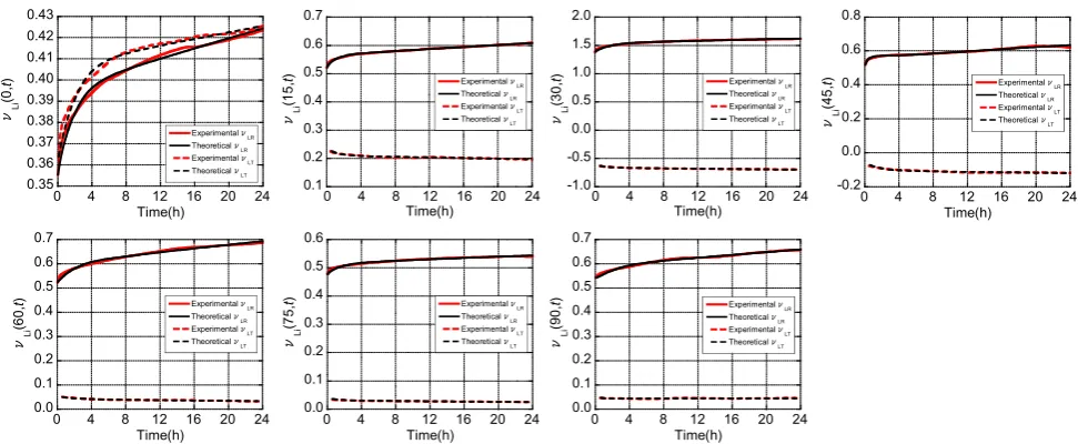
Fig. 13 Progression of viscoelastic Poisson’s ratios mLi(a, t) for Japanese cypress. i=R or T.Solid line mLR(a, t), dotted linemLT(a, t).

Theoretical values were obtained from the model in Fig.11

0.1 0.2 0.3 0.4 0.5 0.6 0.7

0 4 8 12 16 20 24

Experimental㻌䃜LR Theoretical㻌䃜LR Experimental 䃜LT Theoretical 䃜LT

䃜 Li (1 5 , t ) Time(h) 0.35 0.40 0.45 0.50 0.55

0 4 8 12 16 20 24

Experimental㻌䃜LR Theoretical 䃜LR Experimental 䃜LT Theoretical 䃜LT

䃜 Li (0 , t ) Time(h) -0.2 0.0 0.2 0.4 0.6 0.8 1.0

0 4 8 12 16 20 24

Experimental 䃜LR Theoretical 䃜LR Experimental 䃜LT Theoretical㻌䃜LT

䃜 Li (30 , t ) Time(h) -0.2 0.0 0.2 0.4 0.6 0.8 1.0

0 4 8 12 16 20 24

Experimental 䃜LR Theoretical 䃜LR Experimental㻌䃜LT Theoretical 䃜LT

䃜Li (4 5 , t ) Time(h) 0.0 0.1 0.2 0.3 0.4 0.5 0.6

0 4 8 12 16 20 24

䃜Li (60, t ) Time(h) 0.0 0.1 0.2 0.3 0.4 0.5 0.6

0 4 8 12 16 20 24

Experimental㻌䃜LR Theoretical 䃜LR Experimental 䃜LT Theoretical 䃜LT

䃜Li (7 5 , t ) Time(h) 0.05 0.10 0.15 0.20 0.25 0.30 0.35 0.40 0.45

0 4 8 12 16 20 24

䃜Li (9 0 , t ) Time(h)

Fig. 14 Progression of viscoelastic Poisson’s ratiosmLi(a,t) for Kalopanax.i=R or T.Solid linemLR(a,t),Dotted linemLT(a,t). Theoretical

(11)

coefficients of the dashpots, and stress. From Eqs. (32) and (33), the unknown quantities were calculated by perform-ing regression analyses on the measured longitudinal and transverse strains. The progressions of the creep strains were then predicted using these equations using instanta-neous strain components obtained from experimental measurements. For example, Fig.12shows the regression results of the strains in Japanese cypress at a grain angle of 0°, and the experimental results were found to be in good agreement with the theoretical values from the model. Moreover, the regression curve of the viscoelastic Pois-son’s ratio was derived from the ratio of transverse to longitudinal strains, and the results for Japanese cypress and Kalopanax are presented in Figs.13 and14, respec-tively. Again, the experimental results and theoretical values from the model were found to be in good agreement. Therefore, the eight-element creep model proposed in this study can be used to estimate the viscoelastic Poisson’s ratio at any creep time t. However, this model does not currently have a practical use because many of the quan-tities remain unclear. Further experimental and theoretical works, to determine the unknown quantities (all stiffness moduli of the springs and all viscosity coefficients of the dashpots), are still needed to establish this model.

Conclusions

Through off-axis tensile creep tests on the LT plane of Japanese cypress and Kalopanax specimens, the depen-dence of the Poisson effect in wood on grain angle and creep time was investigated. The Poisson’s ratios reached their extrema around a grain angle of 30°, which was considered to be caused by the influence of shear forces in the L direction of wood. Moreover, the Poisson’s ratio in the LT plane was found to be negative in the range of 15°– 45°. The theoretical Poisson’s ratios were calculated from the theory of orthotropic elasticity, and they were similar to the experimental results in the manner of reaching the re-spective extrema, but the actual values differed.

The progression of the viscoelastic Poisson’s ratio var-ied depending on the grain angle and the measurement plane, and the increment in the viscoelastic Poisson’s ratio after 24 h of creep reached its extremum at a grain angle of around 30°. These trends were also presumed to be caused by the shear forces in the L direction of wood, but further research on the time dependence of the apparent shear modulus GLT(t) is required to understand this influence

more clearly. Taking into account the Poisson effect, an eight-element viscoelastic model was presented, and the progression of viscoelastic Poisson’s ratio under uniaxial creep was well reproduced by this model. However, this

model does not currently have a practical use because many of the quantities remain unclear. Further ex-perimental and theoretical works are still needed to establish this model.

References

1. Hearmon RFS (1948) The effect of grain angle. In: The elasticity of wood and plywood. Forest products research special report No.7. His Majesty’s Stationery Office, London, pp 30–35 2. Kollmann FFP (1968) Mechanics and rheology of wood.

Princi-ples of wood science and technology I: solid wood. Springer, Berlin, pp 292–419

3. Hankinson RL (1921) Investigation of crushing strength of spruce at varying angles of grain. Air Serv Inf Circ 259:3–15

4. Yamai R (1957) On the orthotropic properties of wood in com-pression. J Jpn For Soc 39:328–338

5. Morooka T, Ohgama T, Yamada T (1979) Poisson’s ratio of porous material (in Japanese). J Soc Mater Sci Jpn 28:635–640 6. Ohgama T (1982) Poisson’s ratio of wood as porous material (in

Japanese). Bull Fac Educ Chiba Univ Part II 31:99–107 7. Sliker A, Yu Y (1993) Elastic constants for hardwoods measured

from plate and tension tests. Wood Fiber Sci 25:8–22

8. Reiterer A, Stanzl-Tschegg SE (2001) Compressive behaviour of softwood under uniaxial loading at different orientations to the grain. Mech Mater 33:705–715

9. Liu JY (2002) Analysis of off-axis tension test of wood speci-mens. Wood Fiber Sci 34:205–211

10. Marklund E, Varna J (2009) Modeling the effect of helical fiber structure on wood fiber composite elastic properties. Appl Compos Mater 16:245–262

11. Qing H, Mishnaevsky L Jr (2010) 3D Multiscale microme-chanical model of wood: from annual rings to microfibrils. Int J Solids Struct 47:1253–1267

12. Garab J, Keunecke D, Hering S, Szalai J, Niemz P (2010) Measurement of standard and off-axis elastic moduli and Pois-son’s ratios of spruce and yew wood in the transverse plane. Wood Sci Technol 44:451–464

13. Murata K, Tanahashi H (2010) Measurement of Young’s mod-ulus and Poisson’s ratio of wood specimens in compression test (in Japanese). J Soc Mater Sci Jpn 59:285–290

14. Mascia NT, Nicolas EA (2013) Determination of Poisson’s ratios in relation to fiber angle of a tropical wood species. Constr Build Mater 41:691–696

15. Yoshihara H, Ohta M (1995) Measurement of the in-plane elastic constants of wood by the uniaxial compression test using a single specimen. Mokuzai Gakkaishi 41:218–222

16. Keunecke D, Hering S, Niemz P (2008) Three-dimensional elastic behaviour of common yew and Norway spruce. Wood Sci Technol 42:633–647

17. Jeong GY, Hindman DP (2010) Modeling differently oriented loblolly pine strands incorporating variation of intraring proper-ties using a stochastic finite element method. Wood Fiber Sci 42:51–61

18. Bodig J, Goodman JR (1973) Prediction of elastic parameters for wood. Wood Sci 5:249–264

19. Lakes R (1987) Foam structures with a negative Poisson’s ratio. Science 235:1038–1040

(12)

21. Anderson B, Murphey WK (1970) An investigation of time-de-pendency of Poisson’s ratio in compressively loaded wood. Res Br Sch For Resour Pa State Univ 4:39–41

22. Schniewind AP, Barrett JD (1972) Wood as a linear orthotropic viscoelastic material. Wood Sci Technol 6:43–57

23. Sobue N, Takemura T (1979) Poisson’s ratios in dynamic vis-coelasticity of wood as two-dimensional materials. Mokuzai Gakkaishi 25:258–263

24. Hayashi K, Felix B, Le Govic C (1993) Wood viscoelastic compliance determination with special attention to measurement problems. Mater Struct 26:370–376

25. Frandsen HL, Muszynski L (2006) Modeling of the time and strain dependent Poisson effect in wood and wood-based com-posites. In: Fioravanti M, Macchioni N (eds) Proceeding of the international conference on integrated approach to wood struc-ture, behaviour and applications. Joint meeting of ESWM and COST Action E35. Florence, Italy, 15–17 May 2006, pp 139–144 26. Taniguchi Y, Ando K, Yamamoto H (2010) Determination of three-dimensional viscoelastic compliance in wood by tensile creep test. J Wood Sci 56:82–84

27. Taniguchi Y, Ando K (2010) Time dependence of Poisson’s ef-fect in wood I: the lateral strain behavior. J Wood Sci 56:100–106 28. Taniguchi Y, Ando K (2010) Time dependence of Poisson’s ef-fect in wood II: volume change during uniaxial tensile creep. J Wood Sci 56:350–354

29. Ando K, Mizutani M, Taniguchi Y, Yamamoto H (2013) Time dependence of Poisson’s effect in wood III: asymmetry of three-dimensional viscoelastic compliance matrix of Japanese cypress. J Wood Sci 59:290–298

30. Ozyhar T, Hering S, Niemz P (2013) Viscoelastic characteriza-tion of wood: time dependence of the orthotropic compliance in tension and compression. J Rheol 57:699–717

31. Bodig J, Jayne BA (1982) Orthotropic elasticity. Mechanics of wood and wood composites. Van Nostrand Reinhold, New York, pp 87–126