ABSTRACT : In this paper, we consider a make-to-order supply chain which satisfies demand

(1)

Production -Marketing Coordination under Demand and Lead -Time

Uncertainty

Cuiling Ran Wei He

Management School,University of Shanghai for Science and Technology,Shanghai 200093,China

ABSTRACT: In this paper, we consider a make-to-order supply chain which satisfies demand

that is dependent on both price and quoted lead -time. The manufacturer chooses the lead -time and the order quantity, and the retailer sets the revenue shares. The interactions between

the manufacturer and the retailer are modelled as a Nash Game, and the existence and uniqueness of pure strategy equilibrium are demonstrated. A mechanism that enables the supply chain to coordinate the decisions of the members is developed. Lastly, we also analyze

how the supply chain system parameters impact the optimal supply chain decisions and the supply chain performance.

Keywords: leadtime; demand uncertainty; revenue -sharing contract; production -marketing

coordination

1.Introduction

For many enterprises that provide seasonal customized products or customized products with a life cycle relatively shorter than the replenishment lead time, price and lead -time may be the two

most important decisions. A make-to-order supply chain under dynamic pricing and lead -time [1] has become the main mode of product competition. Therefore, in the coordinated operation of a

centralized supply chain, each node member must consider demand and lead -time parameters as the main factors of decision –making. In reality, product price, manufacturing cost, inventory-related costs, lead-time-related cost, and other important parameters[2-16] in supply

chain operation will vary with market demand uncertainty, so it is necessary to consider demand uncertainty characteristics in the process of supply chain operation. However, each node member

maximizes its own expected profit in the operation of a decentralized supply chain under demand uncertainty or lead -time uncertainty [17-22]. Therefore, in the operation of a centralized supply chain, considering the demand and lead -time uncertainty characteristics of the members will

allow cooperation and optimal performance for the supply chain. In this article, we consider the decisions surrounding a customized product with a short selling season and with demand that is

influenced by both price and lead -time.The contribution of this article is to design a coordination mechanism that enables the supply chain to obtain the optimal decision-making plan.

Petruzzi et al. [1] allowed demand to depend on the order quantity as well as price. Chatterjee et al.[2] discussed delivery guarantees and their relationship with operations and

marketing.M .Sarkar et al. [3] studied the effects of variable production rate and time-dependent holding costs for complementary products in a supply chain model. Li [4] studied a make-to-order

supply chain in, which the demand was influenced by price, quoted lead –time, and quality. Wang

(2)

et al. [5] proposed a government subsidy which coordinated the remanufacturing supply chain for risk-averse manufacturers and retailers. Li and Lee [6] extended the model to an actual supply chain. Webster [7] established a make-to-order model with pricing, lead –time, and capacity

decisions.Liu et al. [8] studied the pricing and lead -time decisions from the whole supply chain perspective.Demand is deterministic and is sensitive to the price and lead -time decisions in these

models. Rao et al. [9]studied a price and lead -time model under random demand. Zhao et al. [10] studied model selection−uniform or differentiated under lead -time and demand uncertainty. Netessine et al. [11] considered operation, management models under demand uncertainty. Allon

et al. [12] showed a Nash equilibrium under expected demand. There is a rapidly growing collection in the literature on lead -time and demand uncertainty [13-19]. The studies in the

literature have incorporated demand uncertainty in the price and lead -time into the model by using queuing systems [20-25]. Song [12] determined price, quoted lead –time, and stock

simultaneously by using queuing systems. Easton and Moodie [13] studied pricing and lead -time decisions for a make-to-order supply chain by using a different approach. So [14,15] found the optimal price and lead -time decisions in a monopolistic setting. The model used in this paper

regarding the selling price and inventory cost is similar to the model of Wu Zhengping et al. [16]. However, the studies mentioned above considered the impact of demand uncertainty or lead

-time uncertainty without the impact of inventory. This paper differs from these studies in that the interactions between the manufacturer and the retailer are modeled as a Nash Game, and the existence and uniqueness of pure strategy equilibrium are demonstrated.We design a revenue -

sharing contract and illustrate how the optimal decision varies with different parameters.

2. Model assumptions and descriptions

We consider a two-echelon supply chain consisting of a manufacturer and a retailer, in which a customized product is produced and sold in a short selling season with uncertain and

price-sensitive demand. The price-sensitive demand can be modeled in an additive fashion. The manufacturer must determine the ordering quantity

q

of a product, selling price

p

, and quoted lead –time

l

for a customized product.

According to modeling needs, some parameters and variables were defined, as shown in Table 1.

TABLE 1: Symbols and their meanings

Symbol Meaning

q

Order quantity

p

Selling price

l

Quoted lead-time

d

Market demand



Noise term

F

( )



Cumulative distribution function (cdf) of



f

( )



Probability density function (pdf) of





Expected demand，cdf

G

_

(.)

, pdf

g

_

(.)

(3)

c

Unit purchasing cost

h

Salvage value

s

Unit penalty cost if

t



l

s

Unit penalty cost if

t



l

h

Unit holding cost if

t



l

t

Lead-time

z

Stocking factor



Profit -sharing ratio

I



Expected profit of the supply chain

M



Manufacturer’s expected profit

r



Retailer’s expected profit



Optimal value Assumptions

(1) The price-sensitive demand

d

has the functional form [9] .

( , )





= +

d p l in the additive demand case, where



( , )p l is the expected demand during the

selling season.

(2) The expected demand is linear in

p

and

l

[8].

( , )



p l = −

 

p−



l

The value



0 is the market potential demand over the selling season, The value



0 is the

price sensitivity factor, The value



0 is the lead -time sensitivity factor.

(3) The noise term



is supported on



A B,



with mean 0, whereA0,B0.

(4) The cumulative distribution function (cdf) of



is

F

( )



, and the probability density function (pdf) of



is

f

( )



.

F

( )



is strictly increasing,

F A

( )

=

0, ( ) 1

F B

=

( i.e., there is always some demand in the market).

(5) The lead-time

T

is affected by the average demand



. Let G t_( ) and g t_( ) denote the lead -time cdf and pdf, respectively.

(6) Inventory-related cost:

c

is the unit purchasing cost. If

d



q

,there is a per-unit holding cost

h

(i.e.,

h



0

is the salvage value, where

h c

+ 

0

);if

d



q

, there is a per-unit short

s

.

( )= ( − )++ ( − )+

C q h q d s d q

where is the expected value operator, and( )l + =max(0, )l .

(7) z= −q



( , )p l is the stocking factor [1] .

( )= ( −



)+ + (



− )+ = ( )+ ( )

(4)

Where ( )=



z( − ) ( )

A

z z x f x dx and ( ) B( ) ( )

z

z x z f x dx

 =



− .

(8) Lead-time-related cost: if

t



l

,there is a holding cost

h

_l per –unit -period; if

t



l

, there is a penalty cost

s

_l per –unit –period.

0

( , )



= _l



l( − ) _( ) + _{l l}



( − ) _( )

C l h l t g t dt s t l g t dt

This depends on



through the lead -time distribution G t_( ).

(9) The random lead –time

t

can be expressed as the product of the expected demand



during the selling season and a random variable that is independent of



[4].



=

t

Where



has pdf



( ) and cdf ( ). From basic statistics, we know that

G t

_

( )

t



= 

and

g t

_

( )

1



( )

t

 

=

.

In the following text,



is the expected profit of the supply chain system, superscript

I

_{denotes the centralized supply chain system, D denotes the decentralized supply chain system,}

ID

denotes the coordinated supply chain system, and



denotes the optimal value．

3.Optimal Decision Model for a Centralized Supply Chain

The centralized supply chain system’s objective is to determine

p q l

, ,

to maximize the expected profit. It is useful to apply a transformation of variables to facilitate the optimization

procedure. Then, p and q are substituted for



and

z

. From the equation

( , )



p l = −

 

p−



l, we can write

  



− −

= l

p (1)

The expected profit of the centralized supply chain can be expressed as

( , , ) ( , ) min( , ) ( ) ( )

( , ) ( , , )

  



  







 − − 

 =_ − _ + + − + −

 

=  −

I l

z l C l z c z C z

l L z l (2)

where

( , )



l

  

l C( , )



l c





 − − 

 =_ − − _

(5)

( , , ) ( ) ( ) l ( , ) ( )

L z



l h c z

  

s C



l c z



 − − 

= +  +_ + − − _

  (4)

( , )



 l represents the system’s profit function, where



is equal to 0, L z( , , )



l is the loss

function, that assesses an overage cost h+c and an underage cost ( )z .

(1

)

( , )

( )

2

I

l

c

h c

s

C l

F z

h c

z



 

 











=

+ + +

−

− +

+

−

− −











（

z,

，）

2

( , )

( )

0

I

l

h

s

C l

f z

z



  









 

= −

+ +

− −

−













（

z,

，）

This implies that



I

( , , )

z l



is concave in

z

for given

p

and

l

. The optimal stocking factor

z

I satisfies the following relationship:

(1

)

( , )

( )= +

2

c

h c

s

 

 

C l



F z

h c







−

− +

+



+ + +

−









Where



= −1( )v , = −

 

+

l l l

s v

s h , and 0( ) ( ) ( ) ( )











 

=h_l



−y y dy+s_l



y− y dy.

Therefore, we can reduce the original optimization problem over three variables to a problem

over the two variables

p

and

l

by first solving for the optimal value

z

as a function of

p

and

l

,then substituting the result back into I( , , )

z



l

 .

The optimal



I ， lI, and I

p satisfy the following relationships:

0 1

( )

2

I I

z



₌



_{+ } 

. (5)

I I

l  =



 . (6)

0 1

( )

2

I I

p p



z



₌ ₋ + _ 

 

  . (7)

Where 0

( ) / (2(1 ))



=

 

− c +

 

+ and 0 0

(



(1

 

) ) /



= − +

p .

4.Optimal Decision Model for a Decentralized Supply Chain

The retailer’s objective is to determine



to maximize the expected profit. The expected profit

of the retailer can be expressed as

max D( ) min( , ) ( ( ))

r

l l

w q d w z



  





 − −   − − 

 =_ − _ =_ − _ − 

(6)

( )

-

1

( )

( , )

2

D

r

w

l

z

z l



  





=

+ 

−



.

( )

2 2

2

0

D r





 

= − 



.

which implies that



D_r

( )



is concave in



for given

z

and

l

. The optimal



satisfies the following relationship:

( , )

-

1

( )

2

D

w l

z l

  

z





=

+ 

. (8)

The manufacturer’s objective is to determine

z

and

l

to maximize the expected profit. The

expected profit of the manufacturer can be expressed as

,

max ( , ) ( ( , )) min( , ) ( )

( ( , ) ) ( ) ( ) ( ( , ) ) ( )

D M

z l z l w C l q d cq C z

w C l c h c z w s C l c z



 = − − −

= − − − +  − + − − 

( , )

(

( ))(

)

( )

D M

l l

z l

z

s

h G l

l





=

− 

+



.

which implies that



D_M

( , )

z l

is concave in

l

. The optimal

l

D satisfies the following relationship:

l

D

( )



=



(9) where

1 l

l l

s

s h



−  

=   ₊ 

  (10)

and

( , ( ))

C

 

l

=



where

0( ) ( ) ( ) ( )

l l

h  y y dy s _ y y dy



=





−



+



 −



Equation (9)and Equation (10) can be substituted with



_MD

( , )

z l

:

( )

(

)

(

) ( ) (

) ( )

D

M

z

w



c



h c

z

w s c



z



=

−

− + 

−

+ − −



.

( )

(

) ( ) (

)

D

M

z

h c

w

F z

w s

c

z





= − + + −

+

+ −

−



.

2 2

( )

(

) ( )

0

D

M

z

h c

w

f z

z



 

= − + + −





.

The optimal stocking factor

z

1

( )

D w s c

z F

h w s







 ₌ −  + − − 

 _{+ + −} 

 . (11)

(7)

system’s optimal decision can be used to derive the unique equilibrium solution.

Proposition. There is at least one Nash Game equilibrium solution in the decentralized

supply chain system. If ( ) 2

  







− − _{+ −   + −} + w A

c w s c w, then the equilibrium

solution is unique.

Proof. The existence of the equilibrium solution can be proved if the reaction function of the

supply chain system’s memberis shown to be a concave function.From Equations (8) , (9)

and (10), the equilibrium solution

z

must satisfy Equation (11).



D is decided uniquely

by

z

D,

l

D is decided uniquely by



D, and

p

D is decided uniquely by



D and



D, if

only one

z

satisfies Equation (11) , the equilibrium solution must then be unique.

Let ( ) ( ( )) ( ) ( )

2

  



 − +   =_ + + − _ − + +   w z

R z w s h F z h c . (s1)

Taking the first- and second-order derivatives of (s1) with respect to

z

,we get

(

)

2

( ) ( ( ))

( ) ( )

2 2

R z w z

w s h f z F z

z

  





   − +  = −_ + + − _ +

 _ + _ + . (s2)

(

) (

2

)

2

2 2

( )

( ) ( )

( ) ( ) 2( ( ))

( ) (2 ) ( )

F z

R z f z

R z r z r z

z f z r z







 ₌ _ ₋ _ ₊

 + . (s3)

If

R z

( )

0

z







,then

R z

( )

is a monotonic function of

z

, so only a unique

z

satisfies

( )

0

R z

=

.Otherwise

R z

( )

=0

z



, and we have

(

) (

2

)

2 2 ( ) 2 0 ( ) ( )

| ( ) 2( ( )) 0

(2 ) ( )

R z z

F z R z

r z r z

z r z





 ₌   _ = − +   +

Equation

R z

( )

=

0

has no more than two solutions, the respective terminal values of which are

( )

(

)

( ( 0 ) ) 2

  



− − = + = − − − +  + w

R B h

A

R s c

c

A w

We can derive that

z

D is the unique solution, if ( ) ( ) 0 2

w A

R A w s c

  



− −

= + − − 

+ .

(8)

From Equation (14) , we can get

p

D







. From Equation (12) , we can get

l

D

 + −

w s c

.

From Equation (11) , we can get ( ) (2



)( ) (

 

)



+ + −

 D  w s c − −

z w .

From Equation (13) , we can get ( )

2

 







− +  + − =  + D

D w z w s c

From the above analysis, we know that s

 

+ −c w , so D

 

l ,if

( ) / (2 )

  



 − + − − +

s c w w A .

Therefore,

R z

( )



0

.

The unique equilibrium solution

z

( ( )) ( ) 2

  



 _{+ + −} − +   _{= +}  ₊    w z

w s h F z h c. (12)

Other equilibrium solutions satisfy the following relationships:

( ) 2

 





− +  = + D

D w z

. (13)



=

D D

l . (14)

 





− −

= D D

D l

p . (15)

5. Revenue-Sharing Contract Design for a Cooperative Supply Chain

Under a revenue-sharing contract, the expected profit of the retailer

( )



ID_r can be described

as ( ) ( ) ( ) ( ) ( , , ) ( ( , ) ) ( ( )) ( ) ID I r

l h c z s z

z l C l c z

z

  



















  − −  +  +    =  =_ _ _− + − _ −  −      .

We can then obtain

( )

1

( , )

(

( ))

(

) ( ))

ID r

l l l

l

C

l

C

l

c

z

s

h





  



 

















− −

=



−



−

− 



+

−

+















2 2 2 3

(

)

( )

2

-

( , )

(

( ))

0

- ( )

ID

l l

r

l

C

l

c

z

l

l s

h

z





  



 













+

 

=

− −

−

− 

 



 













 

.

which implies that



ID_r

( )



is concave in



. The optimal ID ( , )

z l





satisfies the following

(9)

1 ( , )

( , ) ( ( )) ( ) 0

  







  

− − ₋ _{− −} _{− } ₊ ₊ ₋ ₊ _  ₌

   

 

 l l l 

l C l l l

C l c z s s h . (16)

That is,



ID( , )=z l



I.

and we can get ( , , ) (1 ) ( , ) ( ) ( ) ( )

( )

l h c z s z

w z l C l c

z

  











 _{= −}  − − ₊  _{+ +} +  +  

 

  _{− }

   .

Under a revenue-sharing contract, the expected profit of the retailer

( )



ID_r and

manufacturer

( )



_MID can be described as

( )= ( , , )

ID I

r

 

z



l

  .

( , ) (1 ) ( , , )

ID I

M z l



z



l

 = −  .

Next, we use a numerical example to analyze the coordination effect of the revenue-sharingcontract in a supply chain under demand and lead -time uncertainty.

6 A Numerical Example

Suppose we have a two-stage supply chain consisting of a retailer and a manufacturer. The

noise term



follows a uniform distribution,



: U



−1,1



, and the cumulative distribution function (cdf) of



satisfies the following relationship:

0, 1

1

( ) , 1 1

2

1, 1

 − 

 + 

=_ −  



 

x

F x x

x

.

Suppose that random variable



takes a value in the subset [0, ]



，while  =( )t ( / )t



 and

1

( )  / 



₌



−



t t represent the cdf and pdf of



, respectively(



=10，



=2).While it is easy

to find that the optimal expected profit decreases with



, it is difficult to find how the average

demand



 and optimal price

p

 change with



. We conducted numerical experiments and found that a revenue-sharing contract can coordinate the supply chain. A representative example is

reported below in Figures(1--7) and Table 2.The parameters used in this example were

c

=

25

,





( )

w

500(120), 900(210),1300(310)



=

,



= 1 1.5 2 2.5 3 3.5 4 4.5 5 5.5



，，，，，，，，，



,



7, 7.5,8,8.5, 9, 9.5,10,10.5,11,11.5



s

=

,

h

=



3, 3.5, 4, 4.5, 5, 5.5, 6, 6.5, 7, 7.5



,



2, 2.5,3,3.5, 4, 4.5,5,5.5, 6, 6.5



l

s

=

, and

h

l

=



2, 2.5, 3, 3.5, 4, 4.5, 5, 5.5, 6, 6.5



.

(10)

In order to verify the validity of

the

revenue-sharing contract, we first compared the

decision-making results of different supply chains, these are shown in Table 2.

TABLE2: Decision-making results of different supply chain systems

Supply chain system



w





_r



_M



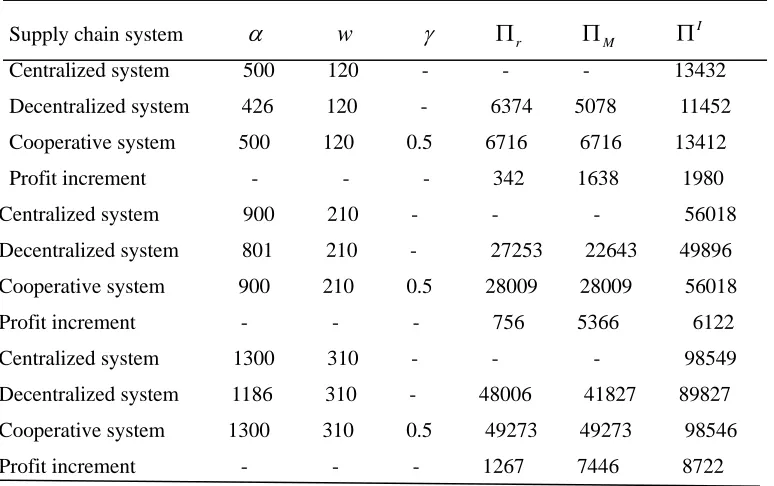
I

Centralized system 500 120 - - - 13432

Decentralized system 426 120 - 6374 5078 11452

Cooperative system 500 120 0.5 6716 6716 13412

Profit increment - - - 342 1638 1980

We compared the decision-making results in Table 2 and found that the revenue-sharing

contract effectively coordinated the supply chain under demand and lead -time uncertainty.The

revenue-sharing contract stimulates the manufacturer’s production behavior and increases the

retailer’s ordering quantity. It can be seen that the revenue-sharing contract increases the profits of

the members of the supply chain. Therefore, the supply chain under demand and lead -time

uncertainty is coordinated by the revenue-sharing contract. In addition, the greater the potential

demand, the more coordination is needed.

6.2Th

e Influence of Parameters on The Optimal Value

Figure 1 shows the influence of the price sensitivity factor



on the optimal stocking

factor

z

. It can be seen that I

z and D

z decrease with increasing



. When the market

potential demand



is relatively small (



=500), I

z and D

z decrease slowly with

increasing



, but when



is relatively large (



=1300), I

z and D

z decrease rapidly with

(11)

1 1.5 2 2.5 3 3.5 4 0.35

0.4 0.45 0.5 0.55 0.6 0.65 0.7

=4, c=25, h=6, s=10, s_l=h_l=6



z

I =500

=900

=1300

(a) centralized supply chain

1 1.5 2 2.5 3 3.5 4

0.55 0.6 0.65 0.7 0.75 0.8 0.85 0.9 0.95

=4, c=25, h=6, s=10, s_l=h_l=6



z

D

=500, w=120

=900, w=210

=1300, w=310

(b) decentralized supply chain

FIGURE 1: The influence of



on z.

1 1.5 2 2.5 3 3.5 4

2 4 6 8 10 12 14 16 18

=4, c=25, h=6, s=10, s_l=h_l=6





I

=500

=900

=1300

1 1.5 2 2.5 3 3.5 4

0 5 10 15 20 25





D

=4, c=25, h=6, s=10, s_l=h_l=6

=500, w=120

=900, w=210

=1300, w=310



on



.

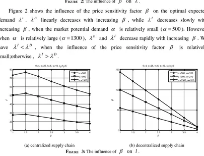
Figure 2 shows the influence of the price sensitivity factor



on the optimal expected

demand



 .



D linearly decreases with increasing



, while



I decreases slowly with increasing



, when the market potential demand



is relatively small (



=500). However, when



is relatively large (



=1300),



D and



I decrease rapidly with increasing



. We have



I





D , when the influence of the price sensitivity factor



is relatively

small;otherwise ,



I





D.

1 1.5 2 2.5 3 3.5 4

10 20 30 40 50 60 70 80



l

I

=4, c=25, h=6, s=10, s_l=h_l=6

=500

=900

=1300

1 1.5 2 2.5 3 3.5 4

0 50 100 150



l

D

=4, c=25, h=6, s=10, s_l=h_l=6

=500, w=120

=900, w=210

=1300, w=310



on l.

(12)

I

l firstly increases and then decreases with increasing



in a centralized supply chain,

while lD decreases rapidly with increasing



in a decentralized supply chain. It can be seen

that a centralized supply chain has a small lead -time with relatively small



, while a

decentralized supply chain has a small lead -time with relatively large



.

1 1.5 2 2.5 3 3.5 4 4.5 5 5.5 0.35 0.4 0.45 0.5 0.55 0.6 0.65 0.7

=4, c=25, h=6, s=10, s_l=h_l=6



z

I _=500

=900 =1300

1 1.5 2 2.5 3 3.5 4 4.5 5 5.5 0.55 0.6 0.65 0.7 0.75 0.8 0.85 0.9  z D

=4, c=25, h=6, s=10, sl=hl=6

=500, w=120 =900, w=210 =1300, w=310



on z.

1 1.5 2 2.5 3 3.5 4 4.5 5 5.5 2 3 4 5 6 7 8 9 10 11

=4, c=25, h=6, s=10, sl=hl=6

  I =500 =900 =1300

1 1.5 2 2.5 3 3.5 4 4.5 5 5.5 0 0.5 1 1.5 2 2.5 3 3.5 4 4.5   D

=4, c=25, h=6, s=10, sl=hl=6

=500, w=120

=900, w=210

=1300, w=310

(b) decentralized supply chian



on



.

1 1.5 2 2.5 3 3.5 4 4.5 5 5.5 10 20 30 40 50 60 70 80  l I

=4, c=25, h=6, s=10, sl=hl=6

=500

=900

=1300

1 1.5 2 2.5 3 3.5 4 4.5 5 5.5 0 5 10 15 20 25 30 35  l D

=4, c=25, h=6, s=10, sl=hl=6

=500, w=120

=900, w=210

=1300, w=310

FIGURE 6:The influence of



on l.

Figures 4 –6 show the influence of the lead -time sensitivity factor



on the optimal decisions.

It can be seen that

z

does not vary with increasing



. The expected demand



decreases

with increasing



in a decentralized or centralized supply chain, so the manufacturer reduces the

(13)

relatively large (



=1300), lIand lD decrease rapidly with increasing



.

l

Idecreases slowly with increasing



in a centralized supply chain, while

l

Ddecreases rapidly with increasing



in a decentralized supply chain. The lead -time in a decentralized supply chain is smaller than the

lead-time in a centralized supply chain.

As shown in Figure 7,



I,



D, lD and lI don’t vary with increasing s and h. Figure

7 also shows that zI and zD increase with increasing s. The penalty cost

s

_l is relatively large, so the manufacturer chooses an ordering quantity in order to avoid shortages. The optimal

stocking factor

z

increases rapidly when the market potential demand



is relatively small; however,when



is relatively large,

z

decreases slowly.

7 7.5 8 8.5 9 9.5 10 10.5 11 11.5 0.25

0.3 0.35 0.4 0.45 0.5 0.55 0.6 0.65 0.7

s

z

I

==4, c=25, h=6, s_l=h_l=6

=500

=900

=1300

7 7.5 8 8.5 9 9.5 10 10.5 11 11.5 0.55

0.6 0.65 0.7 0.75 0.8 0.85 0.9

==4, c=25, h=6, s_l=h_l=6

s

z

D

=500, w=120

=900, w=210

=1300, w=310

FIGURE 7: The influence of s on z.

According to the results of the above numerical analysis, we can draw the following conclusions: Firstly, for different levels of potential demand, the lead -time for the

manufacturer to inform the retailer in a centralized supply chain is much longer than that in a decentralized supply chain.Secondly, the order quantity of customized products in a centralized supply chain is greater than that in a decentralized supply chain. Thirdly, in most

cases,



I





D

,

l

I



l

D, if and only if , the value of



is very small,



I and

l

I will be

less than



D and

l

D respectively.

7.Conclusions

In this paper , we considered a make-to-order supply chain which satisfied demand that

was dependent on both price and quoted lead-time.The manufacturer produced customized products before the selling season. The manufacturer choosed the lead -time and the order quantity, and the retailer set the revenue shares. The interactions between the manufacturer

and the retailer were modelled as a Nash Game and the existence and uniqueness of pure strategy equilibrium were demonstrated.Lastly, we also analyzed how the supply chain system

parameters impacted the optimal supply chain decisions and the supply chain performance. A profit -sharing contract was proposed to coordinate the make-to-order supply chain. In addition, a numerical example was used to analyze how the optimal decision changes with

(14)

decision changed monotonically with most of the parameters. In most cases, the optimal solution of a centralized supply chain was larger than the equilibrium solution of a decentralized supply chain .The analysis in this paper was based on a linear demand function

with an additive form of demand uncertainty. Other demand functions are worthy of investigation.In this paper , we assumed a penalty cost that was independent of the selling

price. It is difficult to address the relationship between the penalty cost and the selling price in our modeling framework; this should be the direction of further research.

Author Contributions: C.R. (Cuiling Ran) and W.H. (Wei He) conceived and designed the

study, C.R. completed the paper in English, W.H. gave many research advices and revised the manuscript. Both of them have read and agreed to the published version of the manuscript.

Funding: This research was supported by the National Natural Science Foundation of China

(no.61803213)

Conflicts of Interest: The authors declare no conflict of interest.

References

[1]. Petruzzi, N .C., K. E. Wee ,M .Dada. A newsvendor model wirth consumer search costs. Prod.

Oper .Manage. 2009, 6, 693-704.

[2]. Chatterjee. S, S. Slotnick, M. Sobel. Delivery guarantees and the interdependence of marketing and operation. Prod. Oper. Manage. 2002, 11, 393-410.

[3]. M. Sarkar, H. Sun, B. Sarkar. Effects of variable production rate and time-dependent holding cost for complementary products in supply chain model. Mathematical Problems in

Engineering. 2017,Article ID2825103,13.

[4]. Li. L. The role of inventory in delivery-time competiton. Manage. Sci. 1992,38, 182-197,

[5]. Wang, K.; Zhao, Y.; Cheng, Y.;Choi, T-M. Cooperation or competition? Channel choice for a

remanufacturing fashion supply chain with government subsidy. Sustainability 2014, 6,

7292–7310.

[6]. Li, L., Y. W. Lee. Pricing and delivery-time performance in a competitive environment. Manage. Sci. 1994, 40, 633-646.

[7]. Webster. S. Dynamic pricing and lead-time policies for make-to –order systems. Decis. Sci. 2002, 33, 579-599.

[8]. Liu. L, M. Parlar, S. X. Zhu. Pricing and lead time decitions in decentralized supply chain. Manage. Sci. 2007, 53, 713-725.

[9]. Rao. U ,J. M. Swaminathan, J. Zhang. Demand and production management with uniform

guaranteed lead time. Prod.Oper. Manage. 2005, 14, 400-412.

[10].Zhao. X, K. E. Stecke, A. Prasad. Lead time and price quotation mode selection:Uniform or

differentiated?. Prod.Oper. Manage. 2012, 14, 400-412.

[11].Netessine. S ,C. Tang. Consumer-driven demand and operation management model: A systematic study of information-technology enabled sales mechanisms. Prod.Oper. Manage.

2013, 14, 400-412.

[12].Allon. G, A. Basssamboo, I. Gurvich. we will be right with you :Managing customer

(15)

decisions under lead-time dependent demand. IIE Transactions. 1998, 13, 151-163. [14].So KC, Song J.. Price, delivery time guarantees and capacity selection. European Journal of

Operational Research.1998, 4, 28-49.

[15].So KC. Price and time competition for service delivery. Manufacturing & Service Operations Management. 2000, 2, 392-409.

[16].Wu Z, Kazaz B, Webster S, Yang K-K. Ordering, pricing, and lead-time quotation under lead-time and demand uncertainty. Pro. Oper.Management. 2012, 21, 576-589.

[17].Tang CS. A review of marketing-operations interfaces models: from co-existence to

coordination and collaboration. Production Economics. 2010, 125, 22-40.

[18].Eliashberg J, Steinberg R. Marketing-production decisions in an industrial channel of

distribution. Management Science. 1987, 33, 981-1000.

[19].Dewan S, Mendelson H, “User delay costs and internal pricing for a service facility”，

Management Science. 1990, l36, 1502-1517.

[20].Porteus E, Whang S. On manufacturing/marketing incentives. Management Science. 1991 , 37, 1166-1181.

[21].Kouvelis P, Lariviere M. Decentralizing cross-functional decisions: coordination through internal markets. Management Science. 2000, 46 ,1049-1058.

[22].Kumar K, Loomba A, Hadjinicola G. Marketing-production coordination in channels of distribution. [J]. Operational Research. 2000, 126, 189-217.

[23].Shan, H.; Zhang, C.; Wei, G. Bundling or Unbundling? Pricing Strategy for Complementry

Products in a Green Supply Chain.Sustainability 2020,12,1331.

[24].Balasubramanian S, Bhardwaj P. When not all conflict is bad: manufacturing- marketing

conflict and strategic incentive design . Management Science. 2004, 50, 489-502.

[25].Pekgün P, Griffin PM, Keskinocak P. Coordination of marketing and production for price and leadtime decisions. IIE Transactions. 2008, 40,12-30.

Creative Commons CC BY