R E S E A R C H
Open Access
Remote sensing classification method of
vegetation dynamics based on time series
Landsat image: a case of opencast mining
area in China
Jiaxing Xu
1,2, Hua Zhao
2, Pengcheng Yin
3, Duo Jia
2and Gang Li
2,3*Abstract
Time series remote sensing image is an important resource for dynamic monitoring of resources and environment, and its abundant time spectrum information can be used to characterize the dynamic change of vegetation coverage. This paper proposes a comprehensive clustering and pixel classification method for extracting the vegetation dynamics based on time series Landsat normalized difference vegetation index (NDVI). This method uses the time-division algorithm for fitting time-series NDVI firstly. And the Markov random field optimized (MRF) semi-supervised dynamic time warping (DTW) kernel fuzzy c-means clustering was constructed. Then the MRF-optimized semi-supervised DTW-kernel fuzzy c-means clustering was combined with the 1-nearest neighbor (1NN) DTW pixel classification to realize the extraction of vegetation dynamics. Shengli Opencast Coal Mine in The Xilin Gol Grassland was taken as the study area to analyze the applicability of the different classification methods. The results showed the fusion algorithm of the MRF-Semi-GDTW-FCM and 1NN-DTW generates accurate classification results with the overall accuracy of 93.8806% and Kappa coefficient of 0.9267, which were 1.7219, 0.0182, and 20.4080% and 0.2916 higher than the clustering and pixel classification, respectively. Experiments proof that the method proposed in this paper is not only simple but also accurate and effective.
Keywords:Vegetation dynamics, Time series NDVI, Classification, Clustering, Pixel classification
1 Introduction
The study on changing processes of land use/land cover is helpful to reveal the response characteristics of envir-onmental factors to envirenvir-onmental change and human intervention. Continuous tracking of dynamic changing information of regional land cover can help reveal the internal mechanism of land use change [1]. At present, it is required that the monitoring of land use change not only can provide the location and direction of the change but also offer corresponding attribute informa-tion to the change, namely effectively identifying the dy-namic land-use category. The remote sensing technology
is characterized in fast, macroscopic, and simultaneous monitoring and provides an efficient and rapid technical method for extracting land-use information. Remote sens-ing time-series images are important resources for dy-namic monitoring of resource and environment and their rich time spectrum information can effectively represent environmental dynamics [2, 3]. The original images are transformed to construct exponential time series and their time spectrums are used to characterize the land-use evo-lution form, which can help reveal the inherent causes and mechanisms of land-use evolution [1,4].
The vegetation growth presents dynamic characteris-tics due to complex changes of external environmental factors. The time series of normalized difference tion index (NDVI), which are used to reflect the vegeta-tion growth status, can effectively record their dynamic process, and their time spectrum meticulously depict the land-use evolution information and make it possible to * Correspondence:[email protected]
2
Key Laboratory for Land Environment and Disaster Monitoring of National Administration of Surveying, Mapping and Geoinformation, China University of Mining and Technology, Xuzhou 221116, China
3Bureau of Land and Resources of Xuzhou, Xuzhou 221006, China Full list of author information is available at the end of the article
identify dynamic vegetation information [5]. Compared with the traditional two-phase image classification, the image time-series analysis can improve the accuracy of information extraction [6]. Huang et al. [7] used Landsat historical data to express the specific spectral index of a disturbance state to construct a time series and pro-posed the Landsat time-series stacks-vegetation change tracker algorithm (LTSS-VCT) for automatic mapping of forest disturbances. Kennedy et al. [8] proposed that the LandTrends time segmentation method was considered to be able to identify the mutation points and trends in the time series of the interannual time series. Verbesselt et al. [9] proposed the breaks for additive season and trend algorithm (BFAST) for real-time remote sensing of ecological disturbance information. For the highly dis-turbed coal mining area, Lei et al. [10] analyzed, with the MODIS-NDVI time series, the temporal and spatial evolution characteristics of vegetation under mining ac-tion in Shendong Mining area. With the deepening of research, many machine learning methods, such as C5.0 decision tree [11], random forest algorithm (RF) [12],
support vector machine (SVM) [13, 14], and fuzzy
c-means clustering [15], are used for extracting dynamic information of the time-series images. Due to big amount of image time-series data, the time spectrum in-formation is susceptible to noise interference, so that the data is subject to high uncertainty and is characterized in seasonality, space-time autocorrelation, etc. [16, 17], which limits the application of many time-series math-ematical models, and the effective mining and classifica-tion methods of image time-series informaclassifica-tion is still faced with many challenges [18, 19]. The extraction of existing time-series information is mostly based on the pixel time series [20], but further studies are required for the disturbance of vegetation phenological difference in different years, the statistical dependence of neighbor-hood pixel and category marking probability, the sensi-tivity of similarity measurement, and how to improve generalization ability of fuzzy classification.
At present, some countries have specially carried out monitoring projects on vegetation disturbances. For ex-ample, as part of the North American Carbon Program project (NACP), the North American Forest Dynamics project (NAFD) made use of Landsat images as the data source and combined ground survey measures to monitor forest disturbances and recovery conditions [21]. The eco-logical and environmental problems brought about by coal mining in China have become increasingly prominent, and the environmental protection situation has become more severe. In areas where mineral resources are con-centrated, land ecological damage and governance have become one of the important issues for sustainable
devel-opment. The “13th Five-Year” Science and Technology
Development Plan for National Environmental Protection
states:“The establishment of a highly developed environ-mental information network, the long-term continuous observation of environmental factors and the mechanism of human activities affecting the Earth system is the trend and demand of current environmental technology devel-opment.”Therefore, based on the image time series, it is of great practical significance to establish a dynamic ex-traction method for the coal mining area.
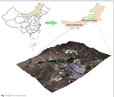
Shengli Opencast Coal Mine is the Mengdong Coal Base, one of Chinese 14 large coal bases. The Xilin Gol Grassland is one of the important grassland areas in China, where the ecological environment is very fragile [10]. The exploitation and utilization of coal resources increases the risk of deterioration of the local ecological environment. Under mining disturbance, the dynamic vegetation information under the mining area is not clear. Although the mining area has undergone eco-logical reconstruction in recent years, there is no rele-vant research on the effect. Taking the Shengli Opencast Mining area as an example, this study is to investigate the consistency of NDVI time series constructed by dif-ferent sensors of Landsat, the correction method of time-series image, and the extraction method of dynamic vegetation information of the opencast mining area based on the interannual Landsat NDVI time series. It is helpful to further enrich the extraction method and the-ory of image time-series information, provide references for the application of image time-series analysis in dy-namic environmental monitoring of the opencast mining area, and establish the scientific theoretical basis for identification of risk sources in the opencast mining area and construction of regional sustainable development and ecological environment.
2 Research area and data
2.1 Research area
put into production and the spatial distribution of all mines is shown in Fig.1.
2.2 Data and preprocessing
L1T data of Landsat TM/ETM+/OLI images from 2000 to 2015, Path 124, Row29, total 160 scenes, were se-lected from the data source: United States Geological Survey (USGS). In order to construct the best image of the growth period, the MODIS16d synthetic data prod-uct (MOD13Q1) from 2000 to 2016 was selected to cal-culate the vegetation growth period in the study area, and the mid-vegetation growth period was used as the middle date of Landsat image synthesis, with the source:
National Aeronautics and Space Administration
(NASA). In order to improve the fitting accuracy, the Google Earth historical images with spatial resolution of
3.7 m in 2010–2011 and the China’s GaoFen-1(GF-1)
multi-spectral images in 2013–2014 were used to assist in judging the time-series trajectory fitting effect. The
spatial location of the mining area boundary, different land-use areas, and working faces was derived from the mining permit boundary of the Shengli Coal Mine and the surface-underground contract plans.
The L1T-level Landsat images provided by the USGS were geometrically corrected by the system up to sub-pixel accuracy without further geometric correction [22]. The Landsat ecosystem disturbance adaptive pro-cessing system (LEDAPS) was carried out for atmos-pheric correction of all Landsat images, to obtain the true reflectivity of the surface and eliminate the pseudo-changes in reflectivity caused by the time-phase
difference between the images [23, 24]. As for the
consistency, difference between the OLI sensor and TM/ ETM+ data, the relative radiation normalization based on ETM+ images was carried out for OLI images in
2013–2014 [25]. In addition, in order to reduce the
function of mask algorithm (FMASK) was used to iden-tify and mask cloud, rain, and shadow [26]. The MODIS NDVI was used to calculate the vegetation growth period in the study area and the middle date (in mid-July) of the growth period was taken as the tie for reflectivity data fusion during the optimal growth period of the vegetation. Then, the time-series trajectory was constructed based on the reflectance data calculation NDVI.
3 Methods
3.1 MRF-optimized semi-supervised DTW-kernel fuzzy c-means clustering
3.1.1 Fuzzy c-means clustering algorithm
Due to the combination of various factors, the time spectrum of the NDVI fitting time series was diverse and had certain uncertainty with the time category. The time spectrum of some types was progressive rather than changing significantly, and the time-spectrum differ-ences between different categories were small, so that the boundaries between classes were fuzzy. The fuzzy c-means clustering algorithm (FCM) introduced the fuzzy membership function into the c-means clustering, to automatically determine the fuzzy partition matrix ac-cording to the relationship between the data. By opti-mizing the objective function, the membership degree of each data to the class center was determined so as to de-cide data attribution [27]. The objective function of the FCM algorithm is:
minJ Uð ;VÞ ¼X
c
i¼1 Xn
j¼1 umijd2ij
s:t:X
c
i¼1
uij¼1;uij∈½0;1;
Xn
j¼1
uij∈ð0;n
ð1Þ
where uij indicates the membership degree that xj
be-longs to class I,U is the membership matrix composed ofuij, V is the class-center matrix formed by cluster
cen-tervi, anddis the Euclidean distance.
3.1.2 DTW Gaussian kernel function
The kernel function is a general method for converting linear classifiers into nonlinear classifiers and the Gauss-ian kernel functions are often used for time series classi-fication. It expresses the similarity between the input time series by calculating the Euclidean distance be-tween the time series of the paired inputs. The scaling between time series and the offset on the time axis cause a certain deviation in the measurement of conventional Euclidean distance, which in turn causes a certain error when the Gaussian kernel function is applied to the time series [28]. The dynamic time warping distance (DTW) allows the time series to be unequal in length and to not
correspond with each other and can be used to effect-ively measure the similarity of the asynchronous time series [29]. Compared with Euclidean distance, DTW is more suitable for expressing time series structures. Therefore, the DTW Gaussian kernel is used as a kernel function [30] and recorded as DTW kernel (GDTW).
K xð ;yÞ ¼ exp Dpðx;yÞ
2
2σ2 !
ð2Þ
Where Dp(x,y) is Sakoe-Chiba-DTW distance of x, y
series.
3.1.3 Semi-supervised DTW-kernel fuzzy c-means clustering
The results of the original FCM clustering are signifi-cantly affected by the initial clustering center. Under the condition of the known number of classifications, the semi-supervised fuzzy c-means clustering is constructed by adding a small amount of prior information to guide the clustering process. According to the optimization theory, the objective function is modified based on the penalty function method, and the DTW kernel metric is used as the measure means of time series similarity to
construct the semi-supervised DTW kernel fuzzy
c-means clustering [31].
3.1.4 Spatial optimization of membership function based on Markov random field
The fuzzy c-means clustering considers only the time di-mension information of the time-series image, but not the statistical dependencies between the neighborhood pixels and the category label probabilities. The Markov random field (MRF) converts Markov property into a planar structure, which combines spatial structures to define probabilistic models on neighborhood systems [32]. Therefore, the spatial optimization scheme of the Markov random field can improve the clustering precision.
3.2 Synthesis of clustering information and pixel classification information
distance, the classification result has greater uncertainty due to the failure to satisfy the conditions of the kernel function [33,34].
The MRF-optimized semi-supervised DTW-kernel fuzzy c-means clustering constructed above is used to fuse with the pixel classification results to realize the synthesis of time spectrum and spatial information, re-move noise, and improve classification homogeneity. The k-nearest neighbor algorithm (KNN) is widely used in information extraction based on similarity measure, but it is more highly sensitive to similarity measure. Many studies have shown that the first neighbor sample has a significant impact on classification accuracy and the 1-nearest neighbor (1NN) algorithm is superior to most complex machine learning algorithms [35]. Based on the KNN algorithm, the 1NN-DTW algorithm uses the DTW distance as the similarity measure and takes k as 1, namely, the first neighbor sample is used to define the pixel label to be classified. Some studies have shown that the 1NN-DTW algorithm is more stable than the KNN algorithm, and has higher stability and classifica-tion accuracy than the DTW Gaussian kernel SVM [20]. Its classification accuracy is even better than most ma-chine learning algorithms [36]. Therefore, the pixel clas-sification is performed by the 1NN-DTW classifier and the Sakoe-Chiba global constraint condition is set for the DTW to prevent the curved path from greatly devi-ating from the diagonal to cause ill-adjustment and affect the classification accuracy. The process for extracting dynamic vegetation information by the fusion
algorithm of the MIR-optimized semi-supervised
DTW-kernel fuzzy c-means clustering and the 1NN-DTW pixel classification is shown in Fig.2.
4 Results and discussion
4.1 Vegetation type division rules
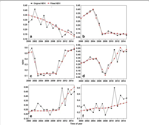
Vegetation changes in coal mining area are affected by multiple factors such as coal mining disturbances, min-ing reclamation, ecological restoration, and so forth. During the monitoring period (2000–2015), the land use in the experimental area gradually changed from natural pasture to industrial and mining land. The large-scale development and construction of the mining area caused a large number of pastures to be disturbed and some areas were restored due to effective reclamation mea-sures. The NDVI time series of the experimental area were divided into six planting dynamic types: continuous disturbance, disturbance-stability, disturbance-stability-recovery, disturbance-disturbance-stability-recovery, smooth-disturbance-stability-recovery, and continuous recovery. The area of the stable zone in the ex-perimental area was small, of which the stability was not considered. Each type recorded the dynamic evolution process of vegetation under the influence of human fac-tors in the experimental area. Manual samples were cali-brated by visual interpretation and the time spectrum and description of each type is as shown in Table1and Fig.3.
4.2 Comparison of clustering accuracy
In order to verify the effectiveness of DTW kernel function (GDTW) and MRF space optimization for
semi-supervised fuzzy c-means clustering, four cluster-ing methods of the semi-supervised FCM (Semi-FCM), the semi-supervised DTW distance (Semi-DTW-FCM), the semi-supervised Gaussian kernel function FCM (Semi-Gaussian-FCM), and the semi-supervised DTW kernel function FCM (Semi-GDTW-FCM) were selected in turn to carry out the clustering for the above test
area. Among the others, the semi-supervised coefficient α was unified to 5, the iterative exit condition ε was
unified to 0.0001, and the initial value of the
Semi-GDTW-FCM kernel parameter was 300. The clus-tering results before and after optimization with MRF space are shown in Fig. 4. The classification results of different models were used to calculate the confusion
Table 1Description of vegetation dynamic types
Vegetation dynamic types Description
Continuous disturbance Vegetation is continuously disturbed during the monitoring period.
Disturbance-stabilization Human activities lead to severe damage to vegetation and there is almost no vegetation cover after disturbance.
Disturbance-stabilization recovery Vegetation is damaged by human disturbance, there is no vegetation, and gradual recovering is carried later.
Disturbance-recovery During the monitoring period, the vegetation began to recover gradually after being disturbed.
Stabilization-recovery During the monitoring period, the vegetation changed from no obvious change to recovery state.
Continuous-recovery Vegetation is in a state of continuous recovery during the monitoring period.
matrix to obtain overall classification accuracy (OA),
Kappa coefficient (Fig. 5), and the differences among
classification results of each model were expressed by error comparison.
As shown in Fig. 4, the spatial information of four
semi-supervised clustering results before and after MRF space optimization is relatively complete, indicating that the semi-supervised clustering model is suitable for the ex-traction of time-series dynamic information. It can be seen from Fig.5that the overall accuracy and Kappa coefficient of four models, namely semi-FCM, semi-DTW-FCM,
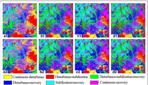
semi-Gaussian-FCM, and semi-GDTW-FCM, are gradually increasing. Among them, the clustering accuracy of semi-DTW-FCM is higher than that of semi-FCM, which indicates that the similarity measure of time series with DTW distance is better than the traditional Euclidean dis-tance. Semi-Gaussian-FCM and semi-GDTW-FCM have higher clustering accuracy than FCM and semi-DTW-FCM, respectively. Therefore, the kernel metrics is used as the measure of similarity to introduce FCM to ef-fectively improve clustering accuracy. In general, the semi-GDTW-FCM has the highest accuracy, indicating that Fig. 4Comparison of MRF spatial structure before and after Optimization.aSemi-FCM.bSemi-DTW-FCM.cSemi-Gaussian-FCM.d Semi-GDTW-FCM. 1 Before the MRF optimization; 2 After the MRF optimization
DTW kernel metrics can be used for FCM algorithm to achieve better clustering results.
The comparison of the results of four models before and after MRF space optimization (Fig.5) shows that the OA and Kappa coefficients after MRF optimization are higher than those before MRF optimization. Among them, the MRF optimization effect of Semi-DTW-FCM and Semi-Gaussian-FCM is more obvious. After MRF optimization, the number of cluster plaques is greatly re-duced while compared with that before optimization and the spatial information expression is more complete than that before MRF optimization. The results show that the MRF spatial structure optimization can effect-ively remove fine plaques, reduce the salt and pepper effect, and improve the classification accuracy by expanding the time dimension to the neighborhood. MRF optimization is more effective in optimizing Semi-DTW-FCM and Semi-GDTW-FCM. After MRF optimization, Semi-GDTW-FCM can achieve the highest clustering accuracy and its OA and Kappa coefficients are 92.1587% and 0.9085, respectively.
4.3 Extraction results and analysis of fusion clustering and pixel classification information
The same experimental data was selected for fusion of clustering and pixel classification information. The MRF-Semi-GDTW-FCM model was used for cluster classifica-tion. The classification accuracy after the fusion of three
typical pixel classification methods based on time series similarity measure (1NN-DTW, Mahalanobis, and spectral angle mapping(SAM)) and MRF-Semi-GDTW-FCM were compared, respectively, and marked as (1NN-MRF-Se-mi-GDTW-FCM, Mahalanobis-MRF-Se(1NN-MRF-Se-mi-GDTW-FCM, and SAM-MRF-Semi-GDTW-FCM), and the degree of in-fluence of different pixel classification accuracy on the
clas-sification accuracy after fusion was analyzed. The
classification results of 1NN-DTW, Mahalanobis, and SAM and their fusions with MRF-Semi-GDTW-FCM were shown in Fig.6, and the confusion matrix was calculated according to the classification results of different models, to obtain overall accuracy (OA) and Kappa coefficient (Table2) after classification.
It can be seen from Fig.6a–c that three classifiers pro-duce a significant “salt and pepper effect” in space. The 1NN-DTW classification accuracy is higher than those of Mahalanobis and SAM, and its classification results main-tain most of the spatial information and are relatively close
to MRF-Semi-GDTW-FCM. It is shown in Table 2 that
the classification accuracy of Mahalanobis and SAM is lower, and the results of MRF-Semi-GDTW-FCM cluster-ing show obvious local misclassification while compared with the above two classifiers. From comparative analysis of Fig. 6 and Table 2, it can be seen that the cation accuracy after the fusion of three pixel classifi-cation methods of 1NN-DTW, Mahalanobis, and SAM with MRF-Semi-GDTW-FCM fusion has been
greatly improved, and OA has increased by 20.4080, 30.5079, and 33.8691%, respectively, and Kappa coeffi-cient has increased by 0.2916, 0.3865, and 0.5651, respectively.
By comparing three pixel classifications fused with
MRF-Semi-GDTW-FCM and MRF-Semi-GDTW-FCM
(Table2), it can be seen that the classification accuracy of 1NN-DTW pixel classification and
MRF-Semi-GDTW-FCM fusion is significantly higher than MRF
-Semi-GDTW-FCM clustering, and its OA and Kappa co-efficients are increased by 1.7219% and 0.0182, respectively, while the classification results of
Mahalanobis-MRF-Semi-GDTW-FCM and SAM-MRF-Semi-GDTW-FCM
have spatially significant “distortion,” the classification ac-curacy is relatively lower than MRF-Semi-GDTW-FCM be-fore fusion, the OA is reduced by 5.1209 and 10.1696%, respectively, and the Kappa coefficient is reduced by 0.1360 and 0.0716, respectively.
In summary, the classification accuracy of the
1NN-DTW pixel classification and
MRF-Semi-GDTW-FCM fusion is higher than that of other classifi-cation methods. The classificlassifi-cation accuracy after fusion is more sensitive to pixel classification and the appropri-ate pixel classification is helpful to improve the classifi-cation accuracy of time series. Compared with SAM and Mahalanobis, 1NN-DTW has higher applicability to time series pixel classification.
5 Conclusions
In allusion to rich local features, noise interference sus-ceptibility, multiple time spectrum shapes, blur inter-class boundary, and other features of the NDVI time series, the fusion of clustering and pixel classification methods can realize the dynamic vegetation information classification in the mining area. The experimental results show that the extraction algorithm of the dynamic vegetation infor-mation of the integrated MRF-optimized semi-GDTW-FCM and the 1NN-DTW pixel classification realizes the integration of time spectrum and spatial information, solves the stretching of time series and the offset of the
time axis, removes fine plaques and noise, improves classification homogeneity, and reduces the“salt and pep-per effect”; compared with other clustering or pixel classi-fication methods, it can improve classiclassi-fication accuracy. The fusion algorithm of the MRF-optimized Semi-GDTW-FCM and the 1NN-DTW pixel classification pro-vides a reliable method and basis for extracting the dy-namic change information of the vegetation in the future and exploring the mechanism of coal resource exploit-ation on the vegetexploit-ation change in coal mining area.
Abbreviations
1NN:1-Nearest neighbor; BFAST: Breaks for additive season and trend; DTW: Dynamic time warping; FCM: Fuzzy c-means clustering; FMASK: Function of mask; GDTW: DTW Gaussian kernel; KNN: k-nearest neighbor; LTSS-VCT: Landsat time-series stacks-vegetation change tracker; MRF: Markov random field; NACP: North American Carbon Program project; NAFD: North American Forest Dynamics project; NDVI: Normalized difference vegetation index; RF: Random forest algorithm; SAM: Spectral angle mapping; SVM: Support vector machine
Acknowledgements
The authors would like to thank the editor, an associate editor, and referees for comments and suggestions which greatly improved this paper.
Availability of data materials
Landsat TM/ETM+/OLI images:http://glovis.usgs.gov/and MODIS (MOD13Q1): https://ladsweb.modaps.eosdis.nasa.gov/
Funding
This research is jointly supported by Land Resources Science and Technology Planning Project of Jiangsu Province (Grant No. 2016028) and Open Foundation of Key Laboratory for Land Environment and Disaster Monitoring of National Administration of Surveying, Mapping and Geoinformation (Grant No. LEDM2014B06).
Authors’contributions
JX and GL conceived and designed the experiments. HZ, PY, and DJ performed the data processing and analysis. JX and GL wrote and modified the manuscript. All authors read and approved the final manuscript.
Ethics approval and consent to participate
Not applicable.
Consent for publication
Not applicable.
Competing interests
The authors declare that they have no competing interests.
Publisher’s Note
Springer Nature remains neutral with regard to jurisdictional claims in published maps and institutional affiliations.
Author details
1The National and Local Joint Engineering Laboratory of Internet Applied Technology on Mines, China University of Mining and Technology, Xuzhou 221008, China.2Key Laboratory for Land Environment and Disaster Monitoring of National Administration of Surveying, Mapping and
Geoinformation, China University of Mining and Technology, Xuzhou 221116, China.3Bureau of Land and Resources of Xuzhou, Xuzhou 221006, China. Table 2Comparison of classification accuracy for fusion of
different pixel classifications and MRF-Semi-GDTW-FCM
Classification method OA (%) Kappa coefficient
1NN-DTW 73.4726 0.6351
Mahalanobis 56.5299 0.386
SAM 48.1200 0.2718
MRF-Semi-GDTW-FCM 92.1587 0.9085
1NN-MRF-Semi-GDTW-FCM 93.8806 0.9267
Mahalanobis-MRF-Semi-GDTW-FCM 87.0378 0.7725
Received: 5 September 2018 Accepted: 16 October 2018
References
1. R.H. Fraser, I. Olthof, M. Carrière, A. Deschamps, D. Pouliot, Detecting long-term changes to vegetationin northern Canada using the Landsat satellite image archive. Environ. Res. Lett.6(4), 045502 (2011).
2. S. Réjichi, F. Châabane, Pixel and region based temporal classification fusion for HR satellite image time series. Geosci Remote Sens Symp133(2), 435– 438 (2012).
3. A. Julea, P. Bolon, C. MP Doin, E.T. Lasserre, V.N. Lazarescu, Unsupervised spatiotemporal mining of satellite image time series using grouped frequent sequential patterns. IEEE Trans. Geosci. Remote Sens.49(4), 1417– 1430 (2011).
4. H. Li, J. Jiang, B. Chen, Y.X. Y Li, W. Shen, Pattern of NDVI-based vegetation greening along an altitudinal gradient in the eastern Himalayas and its response to global warming. Environ Monitor Assess188(3), 1–10 (2016). 5. D.C.S. Djebou, V.P. Singh, O.W. Frauenfeld, Vegetation response to
precipitation across the aridity gradient of the southwestern United States. J. Arid Environ.115(6), 35–43 (2015).
6. J.C. Brown, J.H. Kastens, A.C. Coutinho, D.D.C. Victoria, C.R. Bishop, Classifying multiyear agricultural land use data from Mato Grosso using time-series MODIS vegetation index data. Remote Sens. Environ.130(4), 39–50 (2013). 7. C. Huang, S.N. Goward, J.G. Masek, N. Thomas, Z. Zhu, J.E. Vogelmann, An
automated approach for reconstructing recent forest disturbance history using dense Landsat time series stacks. Remote Sens. Environ.114(1), 183– 198 (2010).
8. R.E. Kennedy, Z. Yang, W.B. Cohen, Detecting trends in forest disturbance and recovery using yearly Landsat time series: 1. LandTrendr—temporal segmentation algorithms. Remote Sens. Environ.114(12), 2897–2910 (2010). 9. J. Verbesselt, R. Hyndman, A. Zeileis, D. Culvenor, Phenological change
detection while accounting for abrupt and gradual trends in satellite image time series. Remote Sens. Environ.114(12), 2970–2980 (2010).
10. S. Lei, L. Ren, Z. Bian, Time-space characterization of vegetation in a semiarid mining area using empirical orthogonal function decomposition of MODIS NDVI time series. Environ Earth Sci75(6), 516 (2016).
11. F. Zhou, A. Zhang, L. Townley-Smith, A data mining approach for evaluation of optimal time-series of MODIS data for land cover mapping at a regional level. ISPRS J. Photogramm. Remote Sens.84, 114–129 (2013).
12. V.F. Rodriguez-Galiano, M. Chica-Olmo, F. Abarca-Hernandez, P.M. Atkinson, C. Jeganathan, Random forest classification of Mediterranean land cover using multi-seasonal imagery and multi-seasonal texture. Remote Sens. Environ.121, 93–107 (2012).
13. B. Zheng, S.W. Myint, P.S. Thenkabail, R.M. Aggarwal, A support vector machine to identify irrigated crop types using time-series Landsat NDVI data. Int. J. Appl. Earth Obs. Geoinf.34(1), 103–112 (2015).
14. X. Zhu, D. Liu, Accurate mapping of forest types using dense seasonal Landsat time-series. ISPRS J. Photogramm. Remote Sens.96(11), 1–11 (2014). 15. T.N. Long, D.S. Mai, W. Pedrycz, Semi-supervising interval Type-2 fuzzy
C-means clustering with spatial information for multi-spectral satellite image classification and change detection. Comput. Geosci.83, 1–16 (2015). 16. S.K. Maxwell, K.M. Sylvester, Identification of“ever-cropped”land (1984–2010)
using Landsat annual maximum NDVI image composites: Southwestern Kansas case study. Remote Sens. Environ.121, 186–195 (2012).
17. J.N. Hird, G.J. Mcdermid, Noise reduction of NDVI time series: an empirical comparison of selected techniques. Remote Sens. Environ.113(1), 248–258 (2009).
18. R.E. Kennedy, Z. Yang, J. Braaten, C. Copass, N. Antonova, C. Jordan, P. Nelson, Attribution of disturbance change agent from Landsat time-series in support of habitat monitoring in the Puget Sound region, USA. Remote Sens. Environ.166, 271–285 (2015).
19. F. Bovolo, G. Camps-Valls, L. Bruzzone, A support vector domain method for change detection in multitemporal images. Pattern Recogn. Lett.31(10), 1148–1154 (2009).
20. H. Ding, G. Trajcevski, P. Scheuermann, X. Wang, E. Keogh, Querying and mining of time series data: experimental comparison of representations and distance measures. Proceed Vldb Endowm1(2), 1542–1552 (2008). 21. K. Schleeweis, S.N. Goward, C. Huang, J.L. Dwyer, J.L. Dungan, M.A. Lindsey,
A. Michaelis, K. Rishmawi, J.G. Masek, Selection and quality assessment of Landsat data for the North American forest dynamics forest history maps of the US. Int J Digit Earth9(10), 963–980 (2016).
22. J.G. Masek, C. Huang, R. Wolfe, W. Cohen, F. Hall, J. Kutler, P. Nelson, North American forest disturbance mapped from a decadal Landsat record. Remote Sens. Environ.112, 2914–2926 (2008).
23. P. Li, L. Jiang, Z. Feng, Cross-comparison of vegetation indices derived from landsat-7 enhanced thematic mapper plus(ETM+) and landsat-8 operational land imager( OLI) sensors. Remote Sens.6(1), 310–329 (2013).
24. Z. Zhu, Y. Fu, C.E. Woodcock, P. Olofsson, J.E. Vogelmann, C. Holden, M. Wang, S. Dai, Y. Yu, Including land cover change in analysis of greenness trends using all available Landsat 5, 7, and 8 images: a case study from Guangzhou, China (2000–2014). Remote Sens. Environ.185, 243–257 (2016). 25. M.J. Canty, A.A. Nielsen, Automatic radiometric normalization of
multitemporal satellite imagery with the iteratively re-weighted MAD transformation. Remote Sens. Environ.112(3), 1025–1036 (2008). 26. Z. Zhu, C.E. Woodcock, Object-based cloud and cloud shadow detection in
Landsat imagery. Remote Sens. Environ.118, 83–94 (2012).
27. J.C. Bezdek, Pattern recognition with fuzzy objective function algorithms. Plenum Press22(1171), 203–239 (1981).
28. B. Yan, C. Domeniconi,An adaptive kernel method for semi-supervised clustering. 17th European Conference on Machine Learning(2006), pp. 521–532. 29. H. Sakoe, S. Chiba, Dynamic programming algorithm optimization for
spoken word recognition. IEEE Trans. Acoust. Speech Signal Process.26(1), 43–49 (1978).
30. R. Ahmed, A. Temko, W.P. Marnane, G. Boylan, G. Lightbody, Exploring temporal information in neonatal seizures using a dynamic time warping based SVM kernel. Comput. Biol. Med.82, 100–110 (2017).
31. W. Pedrycz, J. Waletzky, Fuzzy clustering with partial supervision. IEEE Trans Syst Man Cybern27(5), 787–795 (1997).
32. L. Bruzzone, D.F. Prieto, Automatic analysis of the difference image for unsupervised change detection. IEEE Trans Geosci Remote Sens38(3), 1171–1182 (2000).
33. Y.S. Jeong, R. Jayaraman, Support vector-based algorithms with weighted dynamic time warping kernel function for time series classification. Knowl.-Based Syst.75, 184–191 (2015).
34. Z. Chen, W. Zuo, Q. Hu, L. Lin, Kernel sparse representation for time series classification. Inf. Sci.292, 15–26 (2015).
35. M. Radovanovic, A. Nanopoulos, M. Ivanovic,Time-series classification in many intrinsic dimensions. 2010 SIAM International Conference on Data Mining(2010), pp. 667–688.
36. Y. D, Y. X, W. A,Making the nearest neighbor meaningful for time series classification. 2011 4th International Congress on Image and Signal Processing