The UDWT image denoising method based on the PDE model of a convexity-preserving diffusion function

R E S E A R C H

Open Access

The UDWT image denoising method based

on the PDE model of a

convexity-preserving diffusion function

Xianghai Wang

, Wenya Zhang

, Rui Li

and Ruoxi Song

Abstract

It is a great challenge to maintain details while suppressing and eliminating noise of the image. Considering the nonconvexity property of the diffusion function and the hypersensitivity of the Laplace operator to noise in the Y-K model, a fourth-order PDE image denoising model (Con_G&L model) is proposed in this paper. This model is constructed by a new convexity-preserving diffusion function which guarantees the corresponding energy functional has a globally unique minimum solution. At the same time, the Gaussian filter is combined with the Laplace operator in this model, and as a result, the noisy image is smoothed before the diffusion process, which improves the ability of capturing the details and edges of the noisy image greatly. Furthermore, by analyzing the statistical properties of the undecimated discrete wavelet transform (UDWT) coefficients of noisy image, we observe that the noise information is mainly distributed in the high-frequency sub-bands, and based on this, the proposed Con_G&L model is applied in the high-frequency sub-bands of the UDWT to get the denoising method. The proposed method removes the image noise effectively with the image texture and other details of the image being maintained. Meanwhile, the generation of false edges and the staircase effect can be suppressed. A large number of simulation experiments verify the effectiveness of the proposed method.

Keywords:Undecimated discrete wavelet transform (UDWT), Fourth-order partial differential equations, Diffuse function, Convexity-preserving, Image denoising

1 Introduction

In the process of image formation and transmission, some noise will be introduced, having a great impact on the subsequent applications. Therefore, effectively sup-pressing and eliminating noise in images has always been a popular research topic in the image processing area. Several of image modeling methods have been proposed to study the relationship between the image background

and the noise component [1–3]. Generally, a good

denoising method should be able to remove the noise from the image while maintaining the information of the edges, contours, and details of the image. In other words, it should remove noise and retain the spatial resolution of the images at the same time.

In recent years, the partial differential equation (PDE) method has become one of the most important

mathematical tools for image modeling and representation due to its good property of flexibility and local adaptabil-ity. Based on the continuous mathematical image model, this kind of method makes the image follow a specified PDE, the processing result of which is considered the ex-pected result [4–6]. In the field of image denoising, the second-order PDE nonlinear diffusion equation (P-M model) proposed by Perona and Malik is a pioneer method in PDE image denoising [7]. This model combines image denoising with edge detection organically and takes into account the preservation of details while denoising. However, in the process of iteration, this model is un-bounded for the boundary detector oscillation when large noise is introduced, and the condition given by the model is smooth, which will affect the results. Also, the model is ill-posed. To tackle these, Alvarez et al. proposed

regular-ized P-M model [8]. However, the regularized model is

not stable when the difference is zero in the diffusion process. Additionally, the diffusion degree is weakened by

© The Author(s). 2019Open AccessThis article is distributed under the terms of the Creative Commons Attribution 4.0 International License (http://creativecommons.org/licenses/by/4.0/), which permits unrestricted use, distribution, and reproduction in any medium, provided you give appropriate credit to the original author(s) and the source, provide a link to the Creative Commons license, and indicate if changes were made.

* Correspondence:[email protected];[email protected]

1_{School of Geography, Liaoning Normal University, Dalian 116029, China}

the first-order partial differential at the edge and texture regions because of the second-order characteristics of the model, and after several iterations, the image gray level will appear as a piecewise constant, and the“block”effect will make it difficult to retain the texture details of the ori-ginal image. To solve these problems, researchers ought to find a PDE model with higher order. The fourth-order PDE model is noted for its stability and computational ef-ficiency. The Y-K model proposed by You and Kaveh in [9] and the LLT model proposed by Lysaker in [10] are some typical models. They efficiently suppress the“block” effect introduced by the second-order PDE model. How-ever, the Y-K model causes an obvious gray difference be-tween some points and their surroundings. In addition, black and white outliers usually emerge in the denoised image. The reason is that the Laplace operator in the model is sensitive to speckle noise, which restrains the dif-fusion of the model. The LLT model is based on the mini-mum L1 norm about the second derivative of the image, and there is a fast computational method of numerical so-lution [11]. Nevertheless, it is essentially a high-order fil-ter, which is more sensitive to the high-frequency information of the image and will inevitably blur the image details and edge information with the diffusion deepening.

The wavelet transform is an effective tool for frequency analysis of signals due to its excellent time-frequency localization ability. Therefore, image denoising methods based on wavelets have frequently been consid-ered. The most typical methods are based on a wavelet

domain, including the general threshold method [12],

extreme threshold method [13], St. Ein unbiased risk

threshold method [14], and Bayesian threshold method

[15–17]. These methods simply and rapidly obtain the corresponding denoising thresholds by using the fre-quency characteristics of decomposing the sub-band co-efficients through image wavelets. However, these methods either have the tendency of “over-stifling” [12, 13] or“over-reserving”[14] the wavelet coefficients. The accuracy of the Bayesian threshold method in estimating the variance of sub-band noise remains to be improved.

Based on the above discussions, in this paper, a novel image denoising method is proposed by the improved Y-K model and UDWT. First, a novel convexity-preserving diffusion function is proposed by introducing the Gauss-ian convolution process to the traditional Y-K model, which ensures the unique minimum solution of the model and decreases the sensitivity of the Laplace opera-tors with respect to speckle noise. Then, the statistical property of noisy image UDWT coefficients is studied; we observe that the noise information is mainly distrib-uted in the high-frequency sub-bands, and based on this, the proposed Con_G&L model is applied in the high-frequency sub-bands of the UDWT to get the denoising

method. A large number of experiments are carried out to verify the effectiveness of the proposed method. The results show that the proposed method can effectively remove the noise in the image while retaining the image edge, texture, and other information details.

The rest of the paper is organized as follows:Section 2 provides the statistical analysis of UDWT coefficient and

gives the proposed denoising model, Section 3gives the

description of the datasets and the details of the experi-ments, and Section4presents the conclusions.

2 Methods

2.1 Statistical analysis of UDWT coefficients of noisy images

The traditional discrete wavelet transform can decom-pose an image to multi-scales and multi-directions. However, due to the downsampling and upsampling process, the wavelet transform is not shift-invariant. To solve this, the undecimated discrete wavelet transform

(UDWT) was proposed by Shensa [18], which not only

retains the properties of wavelet transform, but also has the good property of shift-invariant. UDWT does not utilize the downsampling operation in the process of sig-nal decomposition, and instead, it inserts zeroes every two coefficients to expand the filter in the process of high-pass and pass filtering. The length of low-frequency and high-low-frequency signals obtained by UDWT decomposition is the same as that of the original signal, which not only preserves the time-frequency local characteristics and multiresolution analysis characteris-tics of the wavelet transform but also ensures preserva-tion of the translapreserva-tion invariant characteristics. These characteristics lay a foundation for overcoming the drawbacks of traditional denoising methods and effect-ively suppress the generation of the pseudo-Gibbs phenomenon.

Assuming that the scale function and the wavelet ðϕ;

ψ;ϕ~;ψ~Þare designed by the filterðh;g;~h;~gÞ, UDWT can efficiently decompose the input signalc0into {ω1,⋯,ωJ, cJ} through the following porous algorithm (àtrous) [19],

where ωj (j∈{1, 2,⋯,J}) represents the wavelet

coeffi-cients on the scalejand cJrepresents the wavelet

coeffi-cients on the coarsest resolution:

cjþ1½ ¼l h

j ð Þ

cj

l

½ ¼X

k

h k½ cj lþ2jk

ωjþ1½ ¼l gð Þjcj

l

½ ¼X

k

g k½ cj lþ2jk

8 > > < > >

: ð

1Þ

cj½ ¼l ~h j ð Þ

cjþ1

l

½ þ ~gð Þjωjþ1

l

½ ð2Þ

Since there is no downsampling process, the filter banksðh;g;~h;~gÞonly need to satisfy the complete recon-struction conditions in (3) and do not need to satisfy the de-aliasing conditions.

^

hð Þvb~h vð Þ þ^gð Þvb~g vð Þ ¼1 ð3Þ

Furthermore, the above porous algorithm can be ex-tended to two-dimensional image decomposition in the following two-dimensional tensor product form:

cjþ1½ ¼k;l h

j

ð Þ hð Þjcj

k;l

½ ; w1jþ1½ ¼k;l g

j

ð Þ_hð Þj cj

k;l

½

w2

jþ1½ ¼k;l h

j

ð Þ gð Þj_c

j

k;l

½ ; w3

jþ1½ ¼k;l gð Þjgð Þjcj

k;l

½

8 < :

ð4Þ

wherehg∗cis the convolution performed with separable filters hg, which means being convolved with h by col-umn and then withgby row. Three detailed scale images

w1, w2, and w3 are obtained at each scale, which have the same size as the original image.

To study the distribution of noise coefficients of the noisy images after UDWT transform, we use the maximum likeli-hood estimation (ML) method shown in (5) to obtain the variance estimation of each noisy observation sub-band [20]:

^ σ2

y¼

1

nn

X

i

y2_{ð Þi ð5Þ}

wheren×nis the size of sub-band andyis the observed image.

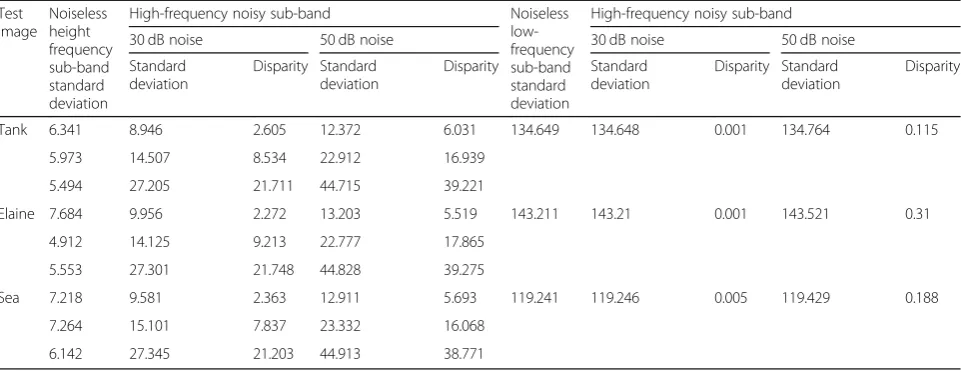
In this paper, Tank, Elaine, and Sea (512 × 512, 8 bpp) are used as test images (see Fig. 1); Gaussian white noise with a mean value of 0 and variance of 30 dB and 50 dB are added using MATLAB. At the same time, three-layer UDWT decomposition is performed for the original image and noisy image, and three high-frequency sub-bands and one low-frequency sub-band are obtained. The standard

deviation statistics about the low-frequency sub-bands and high-frequency sub-bands of the two kinds of images are given in Table1.

As seen in Table1, after decomposition by UDWT, the

noise mainly distributes in the coefficients of the high-frequency sub-bands and the standard deviation of the low-frequency sub-band coefficients of the noisy images, and the images without noise are very close. That is, the influence of noise on the low-frequency sub-band of UDWT coefficients is very small. Hence, in the process of improved PDE model image denoising based on UDWT, we only need to deal with the high-frequency sub-band and keep the low-frequency sub-band state unchanged. In this way, we can improve the computation efficiency of diffusion and avoid the tendency of“over-strangling” the approximation sub-band coefficients.

2.2 Proposed PDE model of the convexity-preserving diffusion function

2.2.1 Analysis of Y-K model

For a continuous functional in the regionΩ,

E uð Þ ¼

Z

Ωf j∇ 2_uj

dxdy ð6Þ

where ∇2 is the Laplace operator, and when f(⋅)≥0 and f′(⋅) > 0 is satisfied, E(u) reaches its minimum value. The minimum is considered as a variational minimum

problem, and the Euler-Lagrange equation of (6) could

be obtained by the gradient descent method.

∇2_gj∇2_uj∇2_{u¼0 ð7Þ}

whereg(x) =f′(x)/x. According to this, You and Kaveh proposed the Y-K model [4] as (8)

∂u xð ;y;tÞ

∂t ¼−∇

2_gj∇2_uj∇2_u

u xð ;y;0Þ ¼u0ðx;yÞ

(

ð8Þ

where ∇2u¼∂_∂2_xu2þ∂ 2_u

∂y2, u0(x,y) is the original image,

u(x,y,t) is the image after smoothing, and u0(x,y) is

in the time scale t, and we select gðsÞ ¼_1þð1

s=kÞ2 as dif-fusion coefficient, where k is the edge threshold (constant).

The Y-K model reduces the block effect of low-order PDE models in the image denoising process and achieves a good balance between removing noise and preserving edges. However, in the process of denoising, the Y-K model will produce a “speckle” effect, which leads to secondary contamination of the image. The reasons are as follows:

The energy functionalE(u) of (6) has the same concav-ity and convexconcav-ity with f(⋅), and if f(⋅) is a convex func-tion, we can know f′(s)≥0 andf″(s)≥0, when ∀s> 0. In

this condition, E(u) has a globally unique minimum

value. However, in the Y-K model, f(⋅) is determined by the selected diffusion function g(s) through f′(s) =sg(s). Overall, we obtain

f0ð Þ ¼s s

1þðs=kÞ2

f″ð Þ ¼s k

2

k2−s2

k2þs2

2

8 > > > < > > > :

ð9Þ

Clearly,f″(s) < 0 whens>k, which meansf(⋅) is no lon-ger guaranteed to be convex. Therefore, it is not guaran-teed thatE(u) has a globally unique minimum solution.

2.2.2 Construction of the model

For the nonconvexity of the diffusion function in the Y-K model, a new convexity-preserving diffusion function is constructed. Considering that the functional purpose of the diffusion function in the Y-K model is to detect edge infor-mation in images and that the Laplace operator∇2is very sensitive to noise, it is difficult to detect edge information effectively in noisy images. For this reason, we combine the

Gaussian filter with the Laplace operator, and Gaussian smoothing is performed before edge detection using the constructed convexity-preserving diffusion function. Based on this smoothing, an image diffusion denoising model (named Con_G&L) is proposed, combining the constructed convexity-preserving diffusion function with the Gaussian filter and Laplace operator. The specific form is

∂u xð ;y;tÞ

∂t ¼−∇

2 _g

Convexðj∇2ðGσuÞjÞ∇2u

u xð ;y;0Þ ¼u0ðx;yÞ

(

ð10Þ

whereGσðÞ ¼pffiffiffiffiffiffi_2πσ1 expð−jj

2

2σ2Þis a Gaussian convolution

kernel with variance σ(σ> 0), ⊗ is the two-dimensional convolution operation, ∇2is the Laplace operator, u0(x,

y) is the original image, andu(x,y,t) is the image after smoothing in the time scale t, gConvex(⋅) is the diffusion

function proposed whose specific form is

g_Convexð Þ ¼s ffiffiffiffiffiffiffiffiffiffiffiffiffiffiffiffiffiffiffiffiffiffiffi1

1þðs=kÞ2p

q ;p∈ð0; 1;s>0: ð11Þ

Here, k is the threshold parameter to distinguish the

edges and smooth areas of the image. If the value ofkis too small to distinguish the noise points well, it is prone to a step effect. If the value of kis too large, the image will be blurred by excessive denoising. To increase the locally adaptive property, according to [21], k is set as

k= 1.4826 × median‖(|∇2u|−median(|∇2u| ))‖.

Furthermore, g(s) is a nonnegative monotonously de-creasing function, which satisfies

g_Convexð Þ ¼0 1; lim

s→∞gConvexð Þ ¼s 0: ð12Þ

In addition, p∈(0, 1] is the regulatory factor. The larger thep is, the faster the function gConvex(s) decreases. Then, Table 1The standard deviation estimate of each sub-band coefficients

Test image

Noiseless height frequency sub-band standard deviation

High-frequency noisy sub-band Noiseless

low-frequency sub-band standard deviation

High-frequency noisy sub-band

30 dB noise 50 dB noise 30 dB noise 50 dB noise

Standard deviation

Disparity Standard deviation

Disparity Standard

deviation

Disparity Standard deviation

Disparity

Tank 6.341 8.946 2.605 12.372 6.031 134.649 134.648 0.001 134.764 0.115

5.973 14.507 8.534 22.912 16.939

5.494 27.205 21.711 44.715 39.221

Elaine 7.684 9.956 2.272 13.203 5.519 143.211 143.21 0.001 143.521 0.31

4.912 14.125 9.213 22.777 17.865

5.553 27.301 21.748 44.828 39.275

Sea 7.218 9.581 2.363 12.911 5.693 119.241 119.246 0.005 119.429 0.188

7.264 15.101 7.837 23.332 16.068

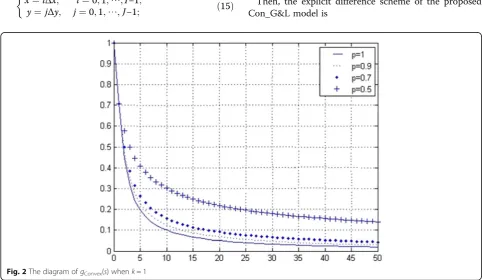
the better the edge information is preserved, the less the noise near the edges is removed. By contrast, the smallerP

is, the slower the function gConvex(s) decreases. Then, the

worse the edge information is preserved, the stronger the noise near the edges is removed. Figure2shows the diagram ofgConvex(⋅) withswhenkis 1 andPis 1, 0.9, 0.7, and 0.5.

Effectiveness analysis of the Con_G&L model is as follows:

Theorem. Based on the diffusion function gConvex(s),

the energy functional E(u) =∫Ωf(|∇2u| )dxdy has a glo-bally unique minimum value.

Proof:For the energy functionalE(u) =∫Ωf(|∇2u| )dxdy,

f(⋅) has the same concave-convex quality. According to the constructed diffusion functiongConvex(s), we setf(⋅) as

∂u xð ;y;tÞ

∂t ¼−∇

2_gj∇2_uj∇2_u

u xð ;y;0Þ ¼u0ðx;yÞ

(

;p∈ð0;1 ð13Þ

Furthermore, we can obtain

f}ð Þ ¼s 1−p

1þðs=kÞ2p

3=2 ð14Þ

due top∈(0, 1], we can knowf' ' (x)≥0. Thus,f(s) is a con-vex function, andE(u) has a globally unique minimum value.

2.2.3 Discretization of the Con_G&L model

In image processing, an image is usually defined as a rectangular field Ω, and it satisfies the following rect-angular network inΩ:

x¼iΔx; i¼0;1;⋯;I−1;

y¼ jΔy; j¼0;1;⋯;J−1; ð15Þ

whereI×J is the size of an image, and we usually select

Δx= 1,Δy= 1 for an image.

Let u(⋅,⋅) be the processed image, u0(⋅,⋅) be the

ori-ginal image, Δt be the time step, h be the space step,

k be the iteration count in this condition, and mark

u(i,j) =ui, j, u0ði;jÞ ¼u0i;j. Taking account of the ac-curacy of calculation, the central difference method is adopted in numerical calculation. The specific calcula-tion format is

uxx ð Þk

i;j¼

uk

iþ1;j−2uik;jþuki−1;j

h2

uyy k

i;j¼

uk

i;jþ1−2uik;jþuki;j−1

h2 ∇2_uk

i;j¼ð Þuxx ki;jþ uyy k

i;j

∇2 _G σu

ð Þk

i;j¼ ðGσuÞxx

k

i;jþ ðGσuÞyy

k

i;j 8

> > > > > > > > > < > > > > > > > > > :

ð16Þ

Let

c∇2u¼g_Convexj∇2ðGσuÞj∇2u

ck_i;j¼c∇2uk_i;j

(

; ð17Þ

we have

∇2_ck i;j¼

ck

iþ1;jþcik−1;jþcki;jþ1þcki;j−1−4cki;j

h2 ð18Þ

Then, the explicit difference scheme of the proposed Con_G&L model is

uk_i;þ_j1¼uk_i;j−Δt∇2ck_i;j: ð19Þ

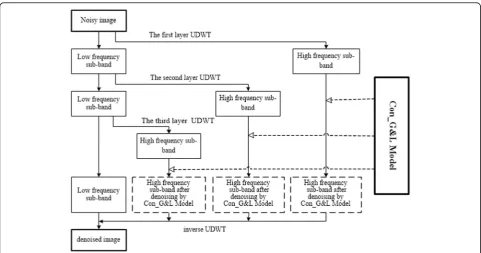
2.3 UDWT image denoising algorithm based on the Con_G&L model

From the analysis and discussion in Section 2.1, it can be seen that noise information is mainly contained in high-frequency sub-bands after UDWT decomposition of the noisy images. Based on that, this paper decom-poses the noisy image into three layers via UDWT and then denoises the three high-frequency sub-bands using the proposed Con_G&L model, while the low-frequency sub-band information remains unchanged. Finally, the final denoised image is obtained by reconstructing the

low-frequency sub-band and the denoised

high-frequency sub-band. The flow chart of the algorithm is shown in Fig.3.

The specific implementation process of the algorithm is as follows:

Step 1. Deal with the noisy images via UDWT.

Step 2. Denoise the high-frequency sub-band components by using the Con_G&L model after UDWT

decomposition.

Step 2.1 calculates 2(Gσ u) of the high-frequency

sub-band and then calculatesgConvex(| 2(G_σ u)| )

according to formula (11).

Step 2.2. Diffuse the Con_G&L model according to

the discrete form (16)–(19).

Step 2.3. Ifjuk_i;þ_j1−uk_i;jj<0:01, proceed to Step 3; otherwise, return to Step 2.1.

Step 3. Apply the inverse UDWT transform for the high-frequency sub-band components after diffusion, which combines the low-frequency sub-band components; then, we obtain the denoised images.

3 Results and discussions

To verify the effectiveness of the proposed algorithm, a large number of simulation experiments have been car-ried out in this paper. The experiment was done with MATLAB (R2018a). The test images are“Elaine,” “Tank,

” “Sea,” “Plane,”and“Panzer”with size 512 × 512. In our experiments, the test images are corrupted by simulated additive noise with a standard deviation equal to 20, 30, 40, 50, and 60, respectively. Besides, we compare our model with the UDWT threshold, LLT, Y-K, and the

denoising method proposed in [22]. The images are

decomposed by three-layer UDWT (filter is db9/7 wave-let), the space stephis 1, the time step Δtis 0.2, and P

is 1. Also, PSNR is used as the objective evaluation index of denoising effect:

PSNR¼10 lg 255

2_mn

Xm

i¼1

Xn

j¼1

uð Þi;j −u0ð Þi;j

2 ð

20Þ

where u∗(⋅,⋅) is the denoised image, u0(⋅,⋅) is the

noiseless original image, m is the length of the image, andnis the width.

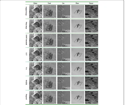
Figure4shows the denoising results of five test images after adding Gaussian white noise with a variance of 30.

Figure 5 is the denoising results of a local region of

“Sea”when enlarging two times.

Table 2 shows the PNSR statistical results for the five denoised images of the algorithm in this paper and UDWT threshold method, LLT model, Y-K model, and

the denoising method proposed in [22]. All the images

are corrupted with Gaussian white noise with variances of 20, 30, 40, 50, and 60 before denoising.

It can be observed from Figs. 4 and 5 that, compared

with the UDWT threshold method, LLT model method, Y-K model method, and the denoising method proposed in [22], the proposed method is better at maintaining the image texture, edges and details of the information, while

removing noise. It can be seen from Table 2 that our

method achieves superior evaluation indexes in most situ-ations; proposed algorithm has higher PSNR than the other four denoising methods through comparing PSNR values in Table2, especially for high variance noise.

4 Conclusions

As a typical representative of the fourth-order PDE model, the Y-K model can effectively suppress the

“blocky” effect produced by the second-order PDE

model in the process of denoising and achieves a good balance between image denoising and edge preservation. However, the nonconvexity of the diffusion function in the model makes it impossible for the energy function to have a globally unique minimum solution, which results in the “speckle” effect in the process of denoising. In addition, the Laplace operator used in the model is

Fig. 5The comparison of the denoising results of a local region when enlarging two times

Table 2The PSNR of denoising for images of different methods

Image Noise

variance

PSNR (dB) Proposed

Noisy image UDWT threshold LLT Y-K Ref .[22]

Elaine 20 22.13 29.61 29.84 29.64 30.15 30.22

30 18.62 28.67 28.15 28.01 28.94 29.34

40 16.11 27.77 27.21 25.86 28.2 28.35

50 14.13 27.09 24.54 23.86 27.18 27.28

60 12.57 26.63 23.11 21.52 27.23 26.71

Tank 20 22.11 28.47 28.24 28.97 27.42 29.37

30 18.57 27.93 27.23 28.41 26.18 28.64

40 16.09 27.48 24.95 27.18 25.62 27.86

50 14.13 26.85 22.57 25.52 24.88 26.96

60 12.58 25.98 20.31 23.35 24.12 26.17

Sea 20 22.09 28.19 27.72 27.87 29.25 28.29

30 18.61 27.63 27.01 27.48 27.77 27.79

40 16.09 26.82 24.93 25.56 26.86 27.06

50 14.16 26.18 22.62 23.63 26.14 26.31

60 12.59 25.34 20.36 21.69 25.39 25.46

Plane 20 22.12 31.67 30.39 31.45 29.76 31.87

30 18.61 30.51 28.21 28.57 28.85 30.65

40 16.07 29.12 25.48 25.87 27.97 29.31

50 14.14 28.01 22.81 23.69 26.88 28.21

60 12.58 26.91 20.55 21.79 26.14 27.09

Panzer 20 22.12 25.17 26.72 26.78 23.47 26.81

30 18.61 24.91 26.11 26.38 22.04 26.39

40 16.08 24.71 24.25 24.61 21.24 25.86

50 14.14 24.51 22.19 22.84 20.64 25.29

hypersensitive to noise, making it difficult to detect edges in noisy images. Thus, the model loses the transformation and detail information of the image in the process of denoising. In this paper, we construct an image denoising model, Con_G&L, based on a convexity-preserving diffu-sion function and Gaussian convolution. Then, the glo-bally unique minimum solution of the energy functional is guaranteed by the convexity-preserving diffusion function, and the secondary pollution in the denoising process is avoided. At the same time, the ability to recognize details, such as edges in images, is improved by smoothing the Gaussian convolution. Then, an image denoising method based on UDWT and the Con_G&L model is proposed. In this method, the Con_G&L model is applied to deal with the high-frequency sub-band of the UDWT in the noise image, which effectively suppresses the false edges and staircase effect. In short, this method removes the image noise effectively and maintains the image texture and other details at the same time.

Abbreviations

PDE:Partial differential equations; UDWT: Undecimated discrete wavelet transform

Acknowledgements

The authors would like to thank the editor and anonymous reviewers for their helpful comments and valuable suggestions.

Authors’contributions

XW conceived of the study and drafted the manuscript. WZ performed the statistical analysis and drafted the manuscript. RL carried out the design of the algorithm. RS carried out the comparative analysis on the research progress and the existing method. All authors read and approved the final manuscript.

Funding

This research has been funded by the National Natural Science Foundation of China (Grant Nos. 41671439, 41971388) and Innovation Team Support Program of Liaoning Higher Education Department (Grant No. LT2017013).

Availability of data and materials

The authors declare that the data and materials are available.

Competing interests

The authors declare that they have no competing interests.

Author details

1

School of Geography, Liaoning Normal University, Dalian 116029, China.

2_{School of Computer and Information Technology, Liaoning Normal}

University, Dalian 116029, China.3School of Mathematics, Liaoning Normal University, Dalian 116029, China.

Received: 4 April 2019 Accepted: 4 September 2019

References

1. C.G. Yan, H.T. Xie, J.J. Chen, A fast uyghur text detector for complex background images. IEEE Trans. Multimed.20(12), 3389–3398 (2018) 2. C. Yan, L. Li, C. Zhang, B. Liu, Cross-modality bridging and knowledge

transferring for image understanding. IEEE Trans. Multimed..https://doi.org/ 10.1109/TMM.2019.2903448

3. C. Yan, Y.B. Tu, X.Z. Wang, STAT: Spatial-temporal attention mechanism

for video captioning. IEEE Trans. Multimed..https://doi.org/10.1109/TMM. 2019.2924576

4. A. Pandeyand, K.K. Singh, An overview of image denoising and image

denoising techniques. Adv. Res. Electr. Electron. Eng.2, 6_–8 (2015) 5. G.A. Kumar, K. Kusagur,Evaluation of Image Denoising Techniques a

Performance Perspective, International Conference on Signal Processing, Communication, Power and Embedded System(IEEE, Paralakhemundi, 2017), pp. 1836_–1839

6. J.F. Sun, H.Y. Liu, Q. Caiand, A survey of image denoising based on wavelet transform. Boletín Técnico55, 256–262 (2017)

7. P. Perona, J. Malik, Scale space and edge detection using anisotropic diffusion. IEEE Trans. Pattern Anal. Mach. Intell.12(7), 629_–639 (1990) 8. L. Alvarez, P.L. Lions, J.M. Morel, Image selective smoothing and edge

detection by no-linear diffusion. SIAM J. Numer. Anal.29(1), 182–193 (1992) 9. Y.L. You, M. Kaveh, Fourth-order partial differential equation for noise

removal. IEEE Trans. Image Process.9(10), 1723_–1730 (2000)

10. M. Lysaker, A. Lundervold, C. Taix, Noise removal using fourth-order partial differential equation with applications to medical magnetic resonance images in space and time. IEEE Trans. Image Process.12(12), 1579–1590 (2003) 11. T.W. Wang, J.Y. Wen, S.Y. Zhang, B.H. He, H.W. Luo, LLT denoising model

based on fixed-point proximity algorithm. J. Jilin Univ.(Science Edition) 52(4), 794–796 (2014)

12. D.L. Donoho, I.M. Johnstone, G. Kerkyacharian, D. Picark, Wavelet shrinkage: asymptopia. J. R. Stat. Soc. Ser.57, 301_–369 (1995)

13. B. Vidakovic, Statistical modeling by wavelets. Wiley Series in Probability and Statistics: Applied Probability and Statistics. A Wiley-Interscience Publication. (Wiley, New York, 1999), ISBN: 0-471-29365-2

14. T.S. Qu, Y.S. Dai, S.X. Wang, Adaptive wavelet thresholding denoising method based on SURE estimation. Acta Electron. Sin.30(2), 266–268 (2002) 15. F. Abramovich, T. Sapatinas, B.W. Sliverman,Wavelet thresholding via a

bayesian approach [tech.rep.Bristol BS8 1TW](1996)

16. H.X. Wang, A complex wavelet based spatially adaptive method for noised image enhancement. J. Comput. Aided Des. Comput. Graph17(9), 1911–1916 (2005) 17. B. Fu, X.H. Wang, Image denoise algorithm based on inter correlation of

wavelet coefficients at finer scale. Comput. Sci.35(10), 246–249 (2008) 18. M.J. Shensa, Discrete wavelet transform: Wedding the a Trous and Mallat

algorithms. IEEE Trans. Signal Process.40(10), 2464–2482 (1992) 19. M.J. Shensa, The discrete wavelet transform: Wedding the àtrous and

Mallatalgorithms. IEEE Trans. Signal Process40(10), 2464–2482 (1992) 20. J.X. Li, P.L. Shui, Wavelet domain LMMSE-like denoising algorithm based on

GGD ML estimation. J. Electron. Inf. Technol.29(12), 2854–2857 (2007) 21. P.J. Rousseeuw, A.M. Leroy,Regression and Outlier Detection(Wiley, NewYork,

1987), pp. 39–46

22. S. Mukherjee, J. Farrand, W. Yao, A study of total-variation based noise reduction algorithms for low-dose cone-beam computed tomography. Int. J. Image Process.10(4), 188–204 (2016)

Publisher’s Note