www.adv-stat-clim-meteorol-oceanogr.net/3/17/2017/ doi:10.5194/ascmo-3-17-2017
© Author(s) 2017. CC Attribution 3.0 License.
A statistical framework for conditional
extreme event attribution
Pascal Yiou1, Aglaé Jézéquel1, Philippe Naveau1, Frederike E. L. Otto2, Robert Vautard1, and Mathieu Vrac1
1Laboratoire des Sciences du Climat et de l’Environnement, UMR 8212 CEA-CNRS-UVSQ, U Paris-Saclay,
IPSL, Gif-sur-Yvette, France
2Environmental Change Institute, School of Geography and the Environment, University of Oxford,
Oxford, UK
Correspondence to:Pascal Yiou ([email protected])
Received: 13 September 2016 – Revised: 6 March 2017 – Accepted: 14 March 2017 – Published: 18 April 2017
Abstract. The goal of the attribution of individual events is to estimate whether and to what extent the proba-bility of an extreme climate event evolves when external conditions (e.g., due to anthropogenic forcings) change. Many types of climate extremes are linked to the variability of the large-scale atmospheric circulation. It is hence essential to decipher the roles of atmospheric variability and increasing mean temperature in the change of probabilities of extremes. It is also crucial to define a background state (or counterfactual) to which recent observations are compared. In this paper we present a statistical framework to determine the dynamical (linked to the atmospheric circulation) and thermodynamical (linked to slow forcings) contributions to the probability of extreme climate events. We illustrate this methodology on a record precipitation event that hit southern United Kingdom in January 2014. We compare possibilities for the creation of two states (or “worlds”) in which proba-bility change is determined. These two worlds are defined in a large ensemble of atmospheric model simulations (Weather@Home factual and counterfactual simulations) and separate periods (new: 1951–2014, and old: 1900– 1950) in reanalyses and observations. We discuss how the atmospheric circulation conditioning can affect the interpretation of extreme event attribution. We eventually show the qualitative coherence of results between the choice of worlds (factual/counterfactual vs. new/old).
1 Introduction
Many extreme events that occur on a local scale are spe-cific to large-scale atmospheric patterns (e.g., rainfall, wind-storms, heatwaves in Europe, and phases of the North At-lantic Oscillation). If such links have been identified, changes in the probability of local extremes can be due to changes in the properties of the atmospheric circulation or changes in the link between the local variable and the circulation (which can remain unchanged). The first cause is sometimes quali-fied as “dynamic” because it refers to the motion of the atmo-sphere. The second cause is qualified as “thermodynamic” (or “non-dynamic”), because it implicitly assumes that the local variable is related to the local change of atmospheric physical properties (e.g., temperature, water content) in the absence of flow changes (Trenberth et al., 2015).
The extreme event attribution (EEA) consists of estimating if and how the probability of an extreme event depends on the climate forcings (National Academies of Sciences Engineer-ing and Medicine, 2016). One of the outcomes is the assess-ment of whether anthropogenic forcings alter such probabil-ity. This type of study has been used for estimates of liability for extreme events that caused damages (Allen, 2003).
The first scientific challenge of EEA is to define two worlds to be compared. The EEA studies speak of afactual world when all climate forcings (natural and anthropogenic) are considered (Stott et al., 2004; Pall et al., 2011). This is presumably a world that “is”, and in which an event is ob-served with probability p1. Thecounterfactual world
p0. Defining a counterfactual world is a difficult task
be-cause it is a possible but non-observed state of climate. Then, some studies define the fraction of attributable risk (FAR), which is the relative change of probability between the two worlds FAR≡(p1−p0)/p1=1−p0/p1(Stott et al., 2004).
Other combinations of thep0andp1probabilities also
pro-vide pieces of valuable information (Hannart et al., 2016) in the framework of causality theory (Pearl, 2009). The FAR is interpreted in terms of a probability ofnecessarycausation. A probability ofsufficientcausation is defined by 1−1−p1
1−p0.
An alternative approach to factual/counterfactual worlds can be proposed, as in van Haren et al. (2013): a “new” world in which we live, like the recent decades, and an “old” world in which our ancestors lived, like the beginning of the 20th century. We implicitly assume that these two worlds are dif-ferent (at least from the environmental point of view). For instance, the anthropogenic forcings are likely to be stronger in the new world than in the old world. The main feature of this approach is that it can be based on observed data. It is difficult to decipher the natural and anthropogenic forcings between old and new. Moreover, the old world might not be free of anthropogenic forcings. It is just assumed that the old world is less affected than the new world by anthropogenic forcings. Therefore, such an observation-based approach can only provide qualitative information on EEA, from implicit hypotheses in the forcing changes, like “greenhouse gas forc-ing” is larger in the new world than in the old world.
Each of these two approaches can be summarized in terms of a universe containing two worlds (factual/counterfactual or new/old) in which probabilities of extreme events are de-termined.
A second challenge is to determine the dynamical and thermodynamical contributions to the change of probabili-ties of a class of events. We assume that extreme values of a climate variable are generally reached for given patterns of atmospheric circulation. The challenge is (i) to estimate the contribution of atmospheric variability in climate change, and (ii) to determine how the properties of a local climate variable would change if the atmospheric circulation is fixed to these patterns but forcings (natural vs. anthropogenic) are different. This is advocated by a “storyline” approach to de-scribe aclassof extreme events, by understanding the gen-eral synoptic conditions leading to the extremes (Trenberth et al., 2015; Shepherd, 2016). The storyline approach is de-signed to decompose the role of climate change in the dy-namical and thermodydy-namical contributions. From a statisti-cal point of view, this motivates the term “conditional attribu-tion”; we investigate how the probability of a local extreme event that depends on a large-scale atmospheric circulation is affected by global climate change or the properties of the circulation itself. If we focus on precipitation extremes, the issue is to evaluate changes in atmospheric flows leading to high precipitation (the dynamical contribution) and changes in precipitation rates given a favorable atmospheric flow (the
conditional thermodynamical contribution) (Trenberth et al., 2015). This requires one to define a metric to follow the at-mospheric circulation conditioning. We propose two choices of such metrics and evaluate how they affect the interpreta-tion of extreme event attribuinterpreta-tion.
The primary goal of this paper is to propose a statis-tical Bayesian framework to identify dynamical and ther-modynamical contributions to a change of probability of a class of extreme events involving the atmospheric circu-lation. The Bayesian aspect emphasizes the role of atmo-spheric circulation trajectories that drive extreme events. For illustration purposes, we focus on the heavy precipitation event that occurred in Europe in January 2014, which has been investigated by many authors (Huntingford et al., 2014; Matthews et al., 2014; Christidis and Stott, 2015; Schaller et al., 2016). This event was a record precipitation in southern UK and Brittany (France). We test this statistical framework on a combination of two universes (factual/counterfactual and new/old) and two atmospheric circulation metrics. These four experiments allow for a focused discussion on the inter-pretation of extreme event attribution.
Section 2 details the datasets that are used to define two worlds. Section 3 explains the notation and methodology that is developed in the paper. Section 4 gives the results of the analyses from the two datasets. The results are discussed in Sect. 5 and conclusions appear in Sect. 6.
2 Data
This section explains the two universes that are considered in this study. The first one is based on a large ensemble of climate simulations. The second is based on reanalyses and observations.
2.1 Weather@Home
We used an ensemble of atmospheric model simulations from Weather@Home to test factual vs. counterfactual worlds. The Weather@Home data come from the “weather@home” citizen-science project (Massey et al., 2015). This project uses spare CPU time on volunteers’ personal computers to run the regional climate model (RCM) HadRM3P nested in the HadAM3P atmospheric general circulation climate model (AGCM) (Massey et al., 2015) driven with prescribed sea surface temperatures (SSTs) and sea ice concentration (SIC). The RCM covers Europe and the eastern North At-lantic Ocean, at a spatial resolution of about 50 km. These simulations were used by Huntingford et al. (2014) and Schaller et al. (2016) to investigate the impact of climate change on the extreme precipitation of January 2014 in southern UK.
The factual world is made of ≈17 000 winters
(December-January-February: DJF) simulated under
each ensemble member on 1 December to give a different realization of the winter weather.
The counterfactual world is made of ≈117 000 simula-tions with different estimates of condisimula-tions that might have occurred in a world without past emissions of GHGs and other pollutants including sulfate aerosol precursors. The at-mospheric composition is set to the pre-industrial, the max-imum well-observed SIC is used (DJF 1986/1987) and esti-mated anthropogenic SST change patterns are removed from observed DJF 2013/2014 SSTs (Schaller et al., 2016). To ac-count for the uncertainty in the estimates of a world without anthropogenic influence, 11 different patterns are calculated from climate model simulations of the Coupled Model Inter-comparison Project phase 5 (CMIP5) (Taylor et al., 2012).
The circulation C is taken from the sea-level pressure (SLP) data of the RCM simulations. The climate variable R is the southern UK precipitation averaged over land grid points in 50–52◦N, 6.5◦W–2◦E. SimulatedRfor the factual
ensemble members with the wettest 1 % are comparable to observations of January 2014. The mean climate of the RCM has a wet (positive) bias of+0.4 mm day−1in January over southern UK (Schaller et al., 2016) but most RCM simula-tions for January 2014 show smaller anomalies than in the observations reported by Matthews et al. (2014), and show a weaker SLP pattern for the same precipitation anomaly. On average, the factual simulations reproduce a stronger jet stream, compared to the 1986–2011 climatology of Jan-uary 2014 in the North Atlantic, suggesting some potential predictability for the enhanced jet stream of January 2014 (Schaller et al., 2016). The differences in SSTs, SICs and at-mospheric composition between the two sets of simulations lead to an increase (from the counterfactual to factual) of up to 0.5 mm day−1 in the wettest 1 % ensemble members for
January southern United Kingdom precipitation.
2.2 Reanalyses and observations
The comparison of old vs. new worlds was performed with two reanalysis datasets. We consider the circulationC from the SLP over the North Atlantic region (80◦W–50◦E; 25– 70◦N) for both reanalyses. The new world is made of the National Centers for Environmental Prediction (NCEP) re-analysis data for the winters (December to February) be-tween 1951 and 2014 (Kalnay et al., 1996). The old world is made of the 20CR reanalysis dataset for the winters be-tween 1900 and 1950 (Compo et al., 2011). The reason why both reanalyses need to be considered is that 20CR ends in 2011 and hence does not include the winter 2013/2014, in which we are interested, for the case study of Schaller et al. (2016). A few tests on the statistical properties of the circula-tion in both reanalyses were performed on their overlapping period (Schaller et al., 2016). It appears that in spite of us-ing different climate models and with different resolutions, both reanalyses exhibit similar features. This means that the
1900 1920 1940 1960 1980 2000
50
100
150
Year
S
ou
th
er
n U
K
pr
ec
ip
ita
tio
n [
m
m
]
●
Figure 1.Time series of January cumulated observed precipitation in southern United Kingdom between 1900 and 2014 (in mm). The red dot indicates the value ofRfor January 2014.
shift from the old world (with 20CR) to the new world (with NCEP) is rather smooth.
The precipitationR is taken from daily precipitation ob-servations from the UK Met Office (Matthews et al., 2014) between 1900 and 2014. The dataset consists of observa-tions from 14 staobserva-tions in the southern UK. These staobserva-tions include Oxford, Rothamsted, Wisley, Bognor Regis, Cam-bridge, Eastbourne, East Malling, Goudhurst, Hampstead, Hampton, Larkhill, Otterbourne, Shanklin (Isle of White) and Woburn. The variableR is an average of daily values of these 14 stations. We verify that a record of January monthly precipitation was reached in 2014 (Fig. 1).
3 Methodology
3.1 Notations and rationale
We assume that a climate variableR (e.g., temperature, pre-cipitation) and atmospheric circulationC (e.g., SLP, geopo-tential height at 500 hPa) are observed in auniversethat con-tains two distinct worlds that we call W0 and W1. Here,
R is a real variable and C is a two-dimensional field. For the first universe,W1 is the “factual” world andW0 is the
“counterfactual” world. This universe is represented by the Weather@Home ensemble. In the second universeW1is the
new world and W0 is the old world. This universe is
the text the universes to which the worldsWibelong, in order
to avoid unnecessarily complicated notations.
We recall that the W1 worlds (in the two universes) are
close to the one in which we live, either in terms of an-thropogenic/natural climate forcings or in terms of tempo-ral proximity (e.g., the last decades). TheW0worlds contain
only natural climate forcings, or temporal remoteness (e.g., beginning of 20th century: 1900–1950 vs. recent decades: 1951–2014).
We define an extreme event (in either worlds and uni-verses) when a reference threshold Rref for R has been
equalled or exceeded. A “class of events” includes the en-semble of weather types for which the threshold can be equalled or exceeded. In this paper, we assume that such an extreme event is reached during a spell of atmospheric circu-lationCrefin the worldW1.
The goal of extreme event attribution is to determine how the probability of an extreme event differs betweenW1and
W0. Achieving this goal is trivial if a rare event can occur
in one of the worlds and cannot in the other. In practice, this does not happen for most extreme events that have occurred in the past decades, because there are often historical exam-ples of such events (e.g., most European winter storms, Eu-ropean heatwaves). Thus, we assume that a given extreme or rare climate event has a probability of occurrencep1inW1,
andp0inW0.
The probabilitiesp1andp0are defined by
pi=Pr(R(i)> Rref), (1)
where R(i) is the climate variableR in the Wi world, and
i∈ {0,1}.
For obvious pragmatic reasons, we can assume thatp1>
0, because we want to study an event that was observed in the real world. In addition,p1can be fixed to a quantile of the
probability distribution ofRinW1. Here we takep1=0.01
to be consistent with (Schaller et al., 2016). This could be in-terpreted in a one-in-a-century event if the data have a yearly sampling. This defines a class of events (here high values of R). Therefore, there is no uncertainty in the determination of p1. The uncertainty is shifted to the estimate ofRreffromW1
data (if 1/p1is larger than the size ofW1), and inp0.
We want to estimate the ratiop0/p1, determine its
uncer-tainty and investigate how it is controlled by physical factors. These physical factors include changes in the probability dis-tribution of the circulation C betweenW1andW0 and the
changes in the probability distribution ofR ifC is similar inW1 andW0. We introduce the notion of vicinity of
cir-culation trajectories, or theneighborhoodV of an observed circulationCref. The trajectory neighborhood will be defined
in two ways: from the distance to a known weather regime (Sect. 3.3.1), which is computed independently of the event itself, or from the distance to the observed trajectory of cir-culation (Sect. 3.3.2).
3.2 A conditional formulation of extreme event attribution
The probabilitiespi(i∈ {0,1}), which represent the marginal
probability that the climate variableR(i) exceeds a
thresh-oldRref(unconditional on the circulation) in worldWi, can
be decomposed into a product of conditional probabilities involving the atmospheric circulation C(i)∈V(Cref) using
rules of probability (Bayes’ formula) as follows:
pi≡Pr(R(i)> Rref) =Pr(R(i)> Rref|C(i)∈V(Cref))
×Pr(C(i)∈V(Cref))
/Pr(C(i)∈V(Cref)|R(i)> Rref). (2)
The three terms of the right-hand side of Eq. (2) can be computed from data in the two worldsWi.
The ratioρ=p0/p1is then decomposed into three terms
that can yield physical interpretations. The first one is the thermodynamical change between the two worldsfor a given circulation:
ρthe≡Pr(R(0)> Rref|C(0)∈V(Cref))
Pr(R(1)> Rref|C(1)∈V(Cref))
. (3)
In this term, the circulation is fixed to one that is close toCref,
and changes of the probability ofRare due to causes such as an increased temperature (increasing the water availability in the atmosphere, Peixoto and Oort, 1992). If theCrefpattern
is prone to high precipitation, this conditional term allows for a closer focus on the tail of the distribution ofR.
The second term accounts for changes in the patterns of the atmospheric circulation and is hence called “circulation”:
ρcirc≡Pr(C(0)∈V(Cref))
Pr(C(1)∈V(Cref))
. (4)
It is important to note thatCrefis the same in the numerator
and denominator. The circulation term measures the change of likelihood of observing circulation sequences that look likeCref.
The third term is areciprocitycondition for the circulation trajectoryC:
ρrec≡Pr(C(1)∈V(Cref)|R(1)> Rref)
Pr(C(0)∈V(Cref)|R(0)> Rref)
. (5)
This term determines the extent to which the circulation Crefis necessary whenR > Rref. For a fixedRref
precipita-tion rate, it evaluates how likely a circulaprecipita-tion such asCref
is. This reciprocity term allows one to connect the risk-based approach of EEA, based on the study ofρalone (Shepherd, 2016) to the “storyline approach” (Trenberth et al., 2015; National Academies of Sciences Engineering and Medicine, 2016), which involves the processes that drive the extreme precipitation.
term explores the extent to which the circulation is close to the observed one when the cumulated precipitation is high. This multiplicative decomposition of probabilities can be compared with the “additive” decomposition of Shepherd (2016, Eq. 1), who also introduces a non-dynamical term. Our decomposition allows for the fact that the probability distribution of R and C could remain unchanged between
W0andW1, while the physical link between these variables
evolve in compensating ways; the probability of having a highRwhenC is close toCrefcould decrease and the
prob-ability of havingC close toCref whenR is high could
in-crease.
Sampling uncertainties on these three ratios can be deter-mined by bootstrapping over the elements ofWi.
The estimation procedure is the following:
1. determinep1(for example a century return period) and
an empiricalRref(for example fromW1);
2. determine the neighborhood ofCref(for example from
the monthly frequency of a weather regime);
3. determineρthe,ρcirc,ρrecand their sampling distribu-tion for the two worlds, for example by bootstrapping over Wi. The bootstrap is done by repeating random
samples of seasons so that the intra-seasonal coherence is preserved.
We then assess whetherρthe,ρcircandρrecare significantly different from 1 by comparing their sampling distributions. We denoteρ¯the estimate of each ratio from all data. The 5th and 95th quantiles (ρˆ5 %andρˆ95 %, respectively) of the boot-strap simulations provide an interval of the sampling confi-dence interval (ρ¯−(ρˆ95 %− ¯ρ),ρ¯−(ρˆ5 %− ¯ρ))
We will illustrate this approach on the high precipitation event of the winter 2013/2014 in southern UK.
3.3 Circulation neighborhood
In this section, we propose two ways of defining the neigh-borhood of the circulation Cref. This has an impact on the
computation of the thermodynamical and dynamical terms of the decomposition ofρ.
3.3.1 Proximity based on weather regimes
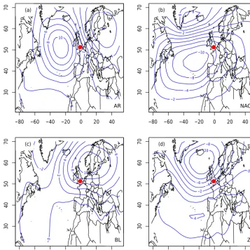
High winter precipitation in Europe is generally associated with zonal atmospheric circulation. The circulation around the North Atlantic can be described by four weather regimes, which are quasi-stationary states of the atmosphere (Vautard et al., 1988; Kimoto and Ghil, 1993; Michelangeli et al., 1995). These weather regimes are obtained by a K means classification of anomalies of the winter SLP daily field from the NCEP reanalysis (Michelangeli et al., 1995; Yiou et al., 2008) on a reference period (1970–2000). The weather regime centroids are shown in Fig. 2.
The weather regimes of the 20CR reanalysis are the same as for NCEP, as well as the regime frequencies (Schaller et al., 2016, supplementary Fig. 7). After a removal of the mean, the SLP of Weather@Home simulations is projected onto these reference centroids to compute the weather regime frequencies. This is done to ensure the consistency of the in-terpretation of the regime frequencies.
The frequencies of the weather regimes are computed for each winter season (December-January-February). Very wet winters in the UK or northwestern France occur when the frequencies of zonal (ZO) or negative phase of the North Atlantic Oscillation (NAO−) weather regimes are high (≥75 %). This threshold duration roughly corresponds to the 97th quantile of frequency for the zonal (ZO) regime in Weather@Home simulations. This allows one to have a non-zero probability of Pr(C(i)∈V(Cref) for the ZO regime
in both reanalysis worlds.
The average frequency of the zonal weather regime is close to 25 % and the frequency reached 81 % in Jan-uary 2014. The two other weather regimes (Scandinavian blocking and Atlantic Ridge) do not lead to very high precip-itation rates in southern UK. The zonal weather regime fa-vors warm temperatures in Europe, while NAO−favors cold temperatures (Yiou and Nogaj, 2004; Cattiaux et al., 2010).
The atmospheric trajectories can then be tracked by daily sequences of weather regimes. We summarize the informa-tion of a trajectory over a whole winter season (or a sin-gle winter month) by the frequencies of the four weather regimes. Hence, ifCrefwas mainly zonal (as was the
win-ter of 2013/2014), we will say that the circulationC is in the neighborhood ofCref (C∈V(Cref)) if the frequency of
the zonal weather regime exceeds 75 %. This definition obvi-ously oversimplifies the notion of circulation neighborhood, but it gives an intuitive and qualitative understanding of the atmospheric circulation. This approach is also taken for con-sistency with the study of Schaller et al. (2016).
3.3.2 Proximity based on analogues of circulation
The computation of weather regimes provides an intuitive and physical interpretation of the atmospheric circulation patterns. But the atmospheric flow trajectories that are con-sidered are, by construction, just closer to one of the weather regime centroids than the others, and not necessarily close to the circulation that prevailed during the event, which could be atypical in terms of weather regimes. Hence, we also ex-plore the atmospheric circulation withanalogues, which ex-ploit explicitly a distance to a reference observed circulation pattern sequence.
IfC(d) is the SLP during some dayd, the analogues of C are the days dk in a different year, for which the
Eu-clidean distanced(C(d), C(dk)) is minimized. This defines
−6
−4
−2
0
0 0 2 4
6
8
10
−80 −60 −40 −20 0 20 40
30
40
50
60
70
●
AR (a)
−10
−8 −6
−4
−2 0
0 2
4 6 8
−80 −60 −40 −20 0 20 40
30
40
50
60
70
●
NAO− (b)
−2
0
0
2 4
6
8
10
−80 −60 −40 −20 0 20 40
30
40
50
60
70
●
BL (c)
−10 −8
−6
−4
−2
0
2
4
−80 −60 −40 −20 0 20 40
30
40
50
60
70
●
ZO (d)
Figure 2. Four winter (DJF) weather regimes of the North Atlantic, computed from the SLP anomalies (in hPa) of NCEP reanalysis.
(a)Atlantic Ridge (AR);(b)NAO−;(c)Scandinavian blocking (BLO);(d)zonal (ZO). The red circles indicate the region where high precipitation was observed.
(2013). We take theK=20 best analogues of circulation for each day.
A justification to use analogues of circulation to describe the January 2014 atmospheric circulation comes from the fact that the SLP had a rather unusual pattern, which did not have all the characteristics of the zonal weather regime shown in Fig. 2. We illustrate this in Fig. 3 with the mean of analogues from W0 (1900–1950 in 20CR; Fig. 3c) and
W1 (1950–2014 in NCEP; Fig. 3d). The mean SLP yields
a rather steep gradient over UK and France. This steep SLP gradient is better reproduced in the analogue mean than in the ZO weather regime.
A heuristic way to define the neighborhood of the trajec-toryCref(e.g., a sequence ofC(d) with days in January 2014)
is to compute the mean (over the days) of a quantile of the distances of the best analogues ofK. This value can be mod-ulated by a “safety” factor to ensure that there are enough trajectories around Cref to construct statistics. This defines
a neighboring “tube” around Cref in the SLP phase space.
This threshold is computed from the analogues ofCrefin
Jan-uary 2014 for the NCEP reanalyses (1950–2014, excluding January 2014) and gives a value of≈12 hPa for a median quantile of theK=20 best daily analogues and a safety fac-tor of 1.5.
In addition to a definition of proximity, we use the dates of the best SLP analogues simulated reconstructions of cli-mate variables. Here we focus on precipitation R. From a statistical perspective, the analogue precipitation is random “replicates” of the precipitation at the day conditioned by the atmospheric circulation. This allows for a determination of the probability distributions of precipitation (R) variability conditioned to the atmospheric circulationC.
Analogues ofC andR provide a natural way of comput-ing the probabilities in Eq. (2). We compute this estimate from the reanalysis datasets (W0=20CR andW1=NCEP).
985
990 995
1000 1005
1005
1010
1015
1020
1020
1025
1025
−80 −60 −40 −20 0 20 40
30
40
50
60
70
●
SLP Jan 2014 (a)
990 995
1000
1005
1005
1010
1015
1020
1020
1020
1020
1025
−80 −60 −40 −20 0 20 40
30
40
50
60
70
●
ZO weather regime (b)
990
995
1000 1000
1005 1010
1015 1020
1020
1025
1025
−80 −60 −40 −20 0 20 40
30
40
50
60
70
●
20CR (W0) SLP analogues (c)
990 995
1000
1005 1005
1010 1015
1015
1020
1020 1020
1025
−80 −60 −40 −20 0 20 40
30
40
50
60
70
●
NCEP (W1) SLP analogues (d)
Figure 3.The mean SLP of January 2014 (in hPa) for(a)NCEP reanalysis(b)ZO weather regime computed from NCEP (Fig. 2d);(c)Mean of analogues in 20CR (1900–1950,W0);(d)Mean of analogues in NCEP (1950–2014,W1). The red circles indicate the region where high precipitation was observed.
in January when random days are drawn inW0=20CR and
W1=NCEP. Hence, the null hypothesis H0 provides an
es-timate of the probability distribution of cumulated random precipitation for January months. We use a Kolmogorov– Smirnov test (von Storch and Zwiers, 2001, p. 81) to ex-amine the difference between the H0 distribution and the circulation-dependent precipitation distribution. We decide to reject H0 at the 1 % level. When comparing the first and second (and third and fourth) box plots, Fig. 4 emphasizes the rejection of this null hypothesis because the distribution of analogue cumulated precipitation probabilities are signifi-cantly higher than for random days. In both cases (NCEP and 20CR), H0 is rejected with a level far below 1 %.
The ρ term is estimated by random resampling of daily R values in January and computing a monthly average. The probability distribution simulations ofRin January 2014 for circulation analogues in W0=20CR and W1=NCEP are
shown in Fig. 4. For comparison purposes, mean precipi-tation taken from random days in the two worlds are also
shown, to emphasize the role of the circulation in the high precipitation event in January. By comparing the second and fourth box plots, Fig. 4 shows a slight increase of the proba-bility of having high precipitation in the new world with re-spect to the old world. The uncertainty onρcan be estimated from these box plots.
The thermodynamical term is estimated from probabilities ofRfor analogues ofCrefinW1andW0. The first step is to
compute analogues ofCref(the circulation in January 2014)
in the two reanalysis datasets. For each day d of January 2014, we draw random circulation analogues inW1andW0,
and keep the sequence of their dates. Then we compute the sum of the analogueR for January 2014. By repeating this procedure, we obtain a Monte-Carlo estimate of the prob-ability distributions of R > Rref conditional to Cref for the
probabil-● ● ● ● ● ● ● ● ● ● ● ● ● ● ● ● ● ● ● ● ● ● ● ● ● ● ● ● ● ● ● ● ● ● ● ● ● ● ● ● ● ● ● ● ● ● ● ● ● ● ● ● ● ● ● ● ● ● ● ● ● ● ● ● ● ● ● ● ● ● ● ● ● ● ● ● ● ● ● ● ● ● ● ● ● ● ● ● ● ● ● ● ● ● ● ● ● ● ● ● ● ● ● ● ● ● ● ● ● ● ● ● ● ● ● ● ● ● ● ● ● ● ● ● ● ● ● ● ● ● ● ● ● ● ● ● ● ● ● ● ● ● ● ● ● ● ● ● ● ● ● ● ● ● ● ● ● ● ● ● ● ● ● ● ● ● ● ● ● ● ● ● ● ● ● ● ● ● ● ● ● ● ● ● ● ● ● ● ● ● ● ● ● ● ● ● ● ● ● ● ● ● ● ● ● ● ● ● ● ● ● ● ● ● ● ● ● ● ● ● ● ● ● ● ● ● ● ● ● ● ● ● ● ● ● ● ● ● ● ● ● ● ● ● ● ● ● ● ● ● ● ● ● ● ● ● ● ● ● ● ● ● ● ● ● ● ● ● ● ● ● ● ● ● ● ● ● ● ● ● ● ● ● ● ● ● ● ● ● ● ● ● ● ● ● ● ● ● ● ● ● ● ● ● ● ● ● ● ● ● ● ● ● ● ● ● ● ●
NCEP H0 NCEP 20CR H0 20CR
0 50 100 150 200 Ja n pr ec ip [m m ]
Figure 4. Box plots of cumulated precipitation simulations (in mm month−1) from circulation analogues of January 2014 from 20CR (1900–1950) and NCEP (1951–2014). The NCEP H0 and 20CR H0 box plots of precipitation are taken from random days in January in 20CR and NCEP (rather than analogues). The horizon-tal thick dashed line is the observed value for January 2014. The horizontal thin dashed line is the 99th quantile of DJF monthly pre-cipitation. The box plot lines indicate the 25th (q25), median (q50)
and 75th (q75) quantile (boxes). The upper whiskers classically
in-dicate min (1.5×(q75−q25)+q50,max(R)). The lower whiskers
have a conjugate formula for low values.
ity distribution ofρthe. In this study, we produceN=1000 random samples ofCand correspondingR.
The dynamical termρdynis obtained by dividingρbyρthe (and using the Bayes formula). This procedure does not give an easy access to the circulation and reciprocity terms be-cause it samples the vicinity ofCref, not all the possible
tra-jectories of SLP, including those which are not close toCref.
4 Results
4.1 Weather@Home
The daily SLP anomalies of the model simulations were clas-sified onto the NCEP reanalysis weather regimes of Fig. 2. For each month, the four weather regime frequencies were computed.
For simplification we pooled all W0 simulations,
un-like Schaller et al. (2016), who investigated each ensem-ble of counterfactual simulations separately. For each of the weather regimes (Atlantic Ridge: AR; zonal: ZO; NAO−; Scandinavian blocking: BLO), we determined the condi-tional probability distribution of January precipitation in southern UK when a weather regime frequency exceeds 75 %
● ● ● ● ● ● ● ●
AR ZO NAO− BLO
0 50 100 150 200 Ja n. p re ci p [m m ] a ● ● ● ● ● ● ● ● ● ● ● ● ● ● ● ● ● ● ● ● ● ● ● ● ● ● ● ● ● ● ● ● ● ● ● ● ● ● ● ● ● ● ● ● ●
AR ZO NAO− BLO
0 50 100 150 200 Ja n. p re ci p [m m ] b
Figure 5. January precipitation probability distribution (box plots) conditional to winter weather regimes exceeding 75 % in Weather@Home simulations (a:W1factual world;b:W0
counter-factual world). The thin dashed horizontal line is the 99 % quantile of theW1(factual) Weather@Home simulations. The thick dashed
horizontal line is the observed precipitation value for January 2014.
of the month. Figure 5 shows that only ZO and NAO−
weather regimes reach the record values observed in January 2014, forW0andW1. A dominant zonal weather regime
ob-viously increases the probability of high precipitation in the winter, although extreme precipitation can also be reached with the NAO−pattern. A visual comparison of the two pan-els of Fig. 5 suggests that the probability of exceeding the 99th precipitation quantile inW1slightly increases fromW0
toW1, because the upper whiskers of the box plots increase.
This visual impression is quantified by the analysis proposed in Sect. 3.2. The fact that precipitation can reach higher val-ues in the counter factual world (Fig. 5b) is due to the fact that W0 contains approximately 7 times more simulations
thanW1.
Figure 5 shows that the North Atlantic circulation patterns are discriminating for heavy precipitation in southern UK. Hence, we focus on the zonal and NAO−atmospheric pat-terns to compute the probability changes.
The difference of high precipitation distribution be-tweenW0andW0is determined by quantile–quantile plots
●●●●●●●●●●●●●●● ●●●●●●●●●●●
● ●●●●●●●
●●●●● ●
● ●
100 120 140 160 180 200
10
0
12
0
14
0
16
0
18
0
20
0
Jan. precip (W0)
Ja
n.
pre
ci
p
(W
1)
a
AR
● ●
●●●●●●●●
●●●●●●●●●●●●●●●●●●●●●●●●●●●●●●●●●●●●●●●●●●●●●●●●●●●●●●●●●●●●●●●●●●●●●●●●●●●●●●●●●●●●●●●●●●●●●●●●●●●●●●●●●●●●●●●●●●●●●●●●●●●●●●●●●●●●●●●●●●●●●●●●●●●●●●●●●●●●●●●●●●●●●●●●●●●●●●●●●●●●●●●●●●●●●●●●●●●●●●●●●●●●●●●●●●●●●●●●●●●●●●●●●●●●●●●●●●●●●●●●●●●●●●●●●●●●●●●●●●●●●●●●●●●●●●●●● ●●●●●●
●●●●●●●● ●●●●●
●● ●
●
100 120 140 160 180 200
10
0
12
0
14
0
16
0
18
0
20
0
Jan. precip (W0)
Ja
n.
p
re
ci
p
(W
1)
b
ZO
●●●●●●●●●●●●● ●●●●●●●●
●●●●● ●●●●●●
●●●●●●●●● ●●●●●●●●●●●●●●●●●
●●●●● ●●●●●
●●●●● ●●
●● ● ●
● ●
100 120 140 160 180 200
10
0
12
0
14
0
16
0
18
0
20
0
Jan. precip (W0)
Ja
n.
p
re
ci
p
(W
1)
c
NAO−
●●●●●●●●●●● ●●●●●●●●●●●●●●●●●●
●●●●●● ●●●●●●●
●●●●● ●
● ●
100 120 140 160 180 200
10
0
12
0
14
0
16
0
18
0
20
0
Jan. precip (W0)
Ja
n.
p
re
ci
p
(W
1)
d
BLO
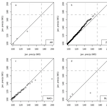
Figure 6. Quantile–quantile plots of January precipitation (in mm month−1) probability distributions between counterfactual (W0) and
factual (W1) worlds in Weather@Home simulations, for each weather regime (a: Atlantic Ridge;b: zonal;c: NAO−;d: Scandinavian blocking). The continuous line is the first diagonal. The thick dashed lines indicate the observation in January 2014. The thin dashed line indicates the 99th quantile of observed January precipitation.
Figure 6b shows that W1 simulations are generally
wet-ter than W1 for the zonal weather regime, apart from one
extreme exception. The precipitation distributions are rather similar for the NAO−weather regime, albeit for an extreme value that far exceeds the observed record (Fig. 6c). The two weather regimes (Atlantic Ridge and Scandinavian blocking) hardly reach the value of the 99th quantile of observed pre-cipitation. Figure 6 hence justifies a posteriori our methodol-ogy to compare the tails of the distributions of precipitation totals. The remainder of the paper focuses on the circulation patterns for which precipitation is likely to exceed the 99th quantile of observations.
The ρ ratios were computed from the (≈17 000) fac-tual and (≈117 000) counterfactual Weather@Home simu-lations. Sincep1is fixed to be 0.01 (for a return period of 1
century), the spread of ρ stems from the uncertainty onp0
that is computed over the pooled counterfactual simulations (although, strictly speaking,Rrefuncertainty depends on the
bootstrap sample fromW1). The distribution ofρis
signifi-cantly different from 1, with a mean valueρ¯=0.71 (Fig. 7, “all” box plot). This indicates an increase of the probabil-ity of heavy precipitation inW1with respect toW0, with a
fraction of attributable risk (FAR=1−p0/p1) of 0.29. This
probability ratio can be decomposed for the ZO and NAO−
weather regimes. The estimates ofρthe,ρcircandρrecfor the ZO and NAO−weather regimes are shown in Fig. 7. By con-struction, the products of the mean values recover the mean value ofρ(all box plot).
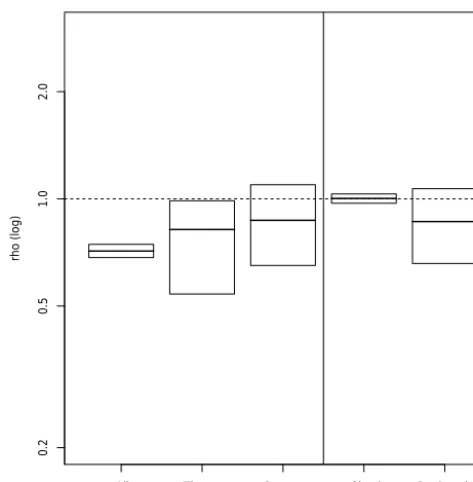
The three mean ratios (ρ¯the, ρ¯circ and ρ¯rec) are signifi-cantly different from 1 for the zonal regime (ρ¯the≈0.63,
¯
ρcirc≈0.78 andρ¯rec≈1.45). Theρthe<1 is interpreted by an increase of precipitation fromW0toW1given the same
weather regime flow.ρcirc<1 reflects an increase of the fre-quency of zonal patterns inW1with respect toW0.ρrec>1
rho (log)
ZO cond.
0.2
0.5
1.0
2.0
All Thermo Dynam Circul Reciprocity
rho (log)
NAO − cond.
0.2
0.5
1.0
2.0
All Thermo Dynam Circul Reciprocity
Figure 7.Changes in probability ratios from weather regimes in Weather@Home simulations. The probability ratios (vertical axes) are shown on a logarithmic scale. The horizonal dashed lines show the referenceρ=1 line. The dynamical contribution is the product of the circulation and reciprocity contributions. The upper panel is the conditional probability ratios for the zonal regime. The lower panel is for the NAO−regime. The thick horizontal segment repre-sents the estimated ratioρ¯from all available data. The boxes repre-sent the bootstrap confidence 90 % intervals (ρ¯−(ρˆ95 %− ¯ρ),ρ¯−
(ρˆ5 %− ¯ρ)), whereρˆ5 %andρˆ95 %are respectively the 5th and 95th quantiles of the bootstrap samples.
The NAO−yields a quite different picture, although it can lead to wet winters in southern UK (Fig. 5). Theρtheratio is not distinguishable from 1 and has a large variability. There-fore, it cannot be concluded that this weather regime has a significant thermodynamic contribution to changes of heavy precipitation rates. ρ¯circ>1 means that the mean January precipitation rate decreases for NAO−fromW0toW1. The
reciprocity ratioρ¯recis lower than 1, meaning that NAO−is less likely during episodes of high precipitation. This means that the NAO−regime becomes less frequent and less rainy, in contradistinction to the zonal regime.
An analogue-like approach was used to estimate the ρ decomposition from the Weather@Home data. The dis-tance between the January 2014 SLP in NCEP and each Weather@Home simulation was computed, as the average of daily SLP distances. Then the neighborhood of Cref=
CJan.2014is defined when this average distance is lower than a
threshold estimated from analogues of NCEP data. The value of the threshold is 1.5 times the average (over January 2014) of the median of the distances of the 20 best daily analogues. This leads to a threshold value of 12 hPa and defines the “cir-culation tube” of Sect. 3.3.2. In this way, the conditional
rho (log)
0.2
0.5
1.0
2.0
All Thermo Dynam Circul Reciprocity
Figure 8. Changes in probability ratios from the analogue ap-proach in Weather@Home simulations. The probability ratios (ver-tical axes) are shown on a logarithmic scale. The horizonal dashed lines show the reference ρ=1 line. The dynamical contribution is the product of the circulation and reciprocity contributions. The boxes yield the same convention as in Fig. 7.
probabilities (and their sampling distributions) can be esti-mated by bootstrapping. The sampling distribution of each probability ratio are shown in Fig. 8.
We see that the thermodynamical contribution is very sim-ilar to the one of the zonal circulation pattern in Fig. 7, but the dynamical contribution has an opposite sign. The circulation contribution is≈1, indicating that the probability of having a circulation like the one of January 2014 does not change sig-nificantly, while the reciprocity term is lowered. Therefore, the frequency of a persisting zonal weather regime increases between the counterfactual and factual worlds, while proba-bility of having a circulation history that is similar to 2014 re-mains stable. This apparent contradiction is explained by the fact that the circulation of January 2014, although zonal, was rather dissimilar to the usual zonal weather regime. Hence, by tightening the class of event from “high precipitation sum due to zonal weather regime” to “high precipitation sum due to a specific persisting circulation”, we change the quantifi-cation of a dynamical contribution.
●
AR ZO NAO− BLO
0
50
10
0
15
0
20
0
P
re
ci
p
D
JF
[m
m
]
NCEP 1950−2014 a
●
AR ZO NAO− BLO
0
50
10
0
15
0
20
0
P
re
ci
p
D
JF
[m
m
]
b 20CR 1900−1950
Figure 9.Cumulated southern UK January precipitation (in mm) probability distribution conditional to winter weather regimes ex-ceeding 75 % in reanalyses (a: NCEP;b: 20CR). The thin dashed horizontal line is the 99 % quantile of W1 (NCEP). The thick
dashed line is the precipitation amount in January 2014.
4.2 Reanalyses
The two reanalyses (20CR and NCEP) use different mod-els, assimilation schemes and assimilated data. Schaller et al. (2016, supplementary information) showed that the weather regime classification in the overlapping period of the two re-analyses are very similar. We also verify that the analogues of January 2014 are qualitatively similar in the two reanalyses over the 1950–2011 period. For each day of January 2014, the 20 best analogues have between 12 and 18 days in com-mon in the two reanalyses. The distances and spatial cor-relation yield probability distributions that cannot be dis-tinguished by a Kolmogorov–Smirnov test (von Storch and Zwiers, 2001).
We set a high threshold of precipitation to the 99th quan-tile of January cumulated precipitation. Due to the rather low number of data points, we also considered the months of De-cember and February during which high cumulated winter precipitation is likely. This choice can also be justified be-cause the properties of the atmospheric circulation are baro-clinic across the winter (Hoskins and James, 2014). We ver-ify that high values of precipitation Rcan be obtained with more than one weather regime (namely, the zonal and NAO−
regimes) in Fig. 9. This justifies that the decomposition of Eq. (2) is repeated for these two weather regimes, although it can be anticipated that this threshold cannot be exceeded for NAO−inW0in the observations.
Again, the North Atlantic circulation patterns are discrim-inating for heavy precipitation in southern UK in the obser-vation universe. Hence, we focus on the ZO and NAO− at-mospheric patterns to compute the probability changes.
Similar estimates ofρ,ρthe,ρcircandρrecwere computed from the NCEP (W1 from 1951 to 2015) and 20CR (W0
from 1900 to 1950) reanalyses (Figure 10). The mean ratio
¯
ρ is≈0.82 ((0.36;1.37) with a 90% confidence interval), indicating a FAR value of ≈0.18. The distribution of ρ is not significantly different from 1 (although the sampling dis-tribution is skewed towards a lower value) due to the low number of observations, but its range is compatible with the Weather@Home estimate.
The three ratio distributions (ρthe, ρcirc and ρrec) were
computed for the zonal and NAO− weather regimes
(Fig. 10). The values cannot be determined for the thermo-dynamical and reciprocity terms because the precipitation threshold is not reached or exceeded inW0 during winters
dominated by NAO−
The mean value is significantly different from 1 for the zonal regime (ρ¯the≈0.36 (0.2, 0.71) for a 90 % confidence interval). They are not significantly different from 1 for the circulation and reciprocity terms ρ¯circ≈0.89 (0.12, 1.34) andρ¯rec≈2.5 (0.2, 4)). This description is qualitatively sim-ilar to what was obtained with the Weather@Home analy-sis for the thermodynamical and dynamical terms, although the magnitudes differ, due to the differences between the two universes (factual vs. counterfactual, and new vs. old). The uncertainty increase is partly due to the limited lengths of the reanalysis datasets. The mean reciprocity ratioρ¯recis rather close to what was found in the Weather@Home analysis. It indicates an increase of zonal circulation when heavy precip-itation occurs between the beginning of the 20th century and the present-day period.
The ρ ratio distributions for the NAO− regime are not very informative. The thermodynamic and reciprocity con-tributions cannot be estimated because the threshold of pre-cipitation is never reached during a winter dominated by NAO− in the NCEP reanalysis, between 1951 and 2014, implying zero denominators in Eqs. (3), (5). A first in-terpretation is that the NAO− regime is so different in both worlds that the conditional precipitation change cannot be estimated (because Pr(R(1)> Rref|C(1)∈V(Cref))=0 and
Pr(C(1)∈V(Cref)|R(1)> Rref)=0). This might be due to the
low number of winters in theW0world (i.e., 50 years).
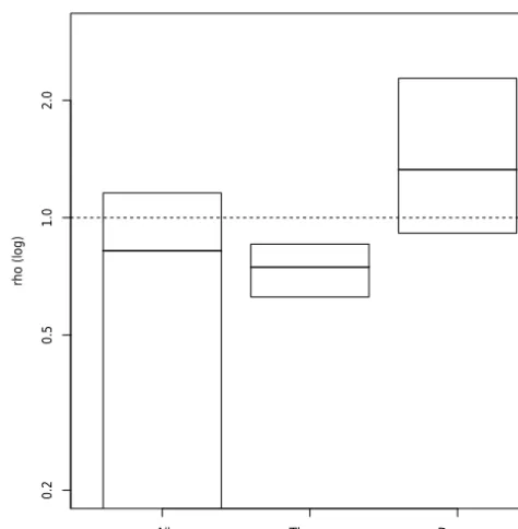
The ratio distributions with the analysis of SLP analogues is shown in Fig. 11. The distribution ofρtheyields a smaller variance than with the weather regime description due to the tighter constraint on the shape of the atmospheric trajectory. The dynamical termρdynis barely above 1 (contrary to the ZO weather regime in the same worlds), although not signif-icantly.
This apparent contradiction is explained by the fact that the ZO weather regime becomes slightly more probable in
rho (log)
ZO cond.
0.2
0.5
1.0
2.0
All Thermo Dynam Circul Reciprocity
rho (log)
NAO − cond.
0.2
0.5
1.0
2.0
All Thermo Dynam Circul Reciprocity
Figure 10. Changes in probability ratios in 20CR/NCEP reanal-yses for the zonal and NAO− weather regimes. The probability ratios (vertical axes) are shown on a logarithmic scale. The hori-zonal dashed lines show the reference ρ=1 line. The dynamical contribution is the product of the circulation and reciprocity contri-butions. The upper panel is the conditional probability ratios for the zonal regime. The lower panel is for the NAO−regime. There are no thermodynamical or reciprocity terms in the decomposition be-cause high precipitation sums do not occur during persisting NAO−
episodes in 1900–1950. The boxes yield the same convention as in Fig. 7.
distance of SLP analogues of January 2014 slightly increases betweenW0andW1(Fig. 12). This reflects the fact that the
January 2014 pattern is not a typical zonal pattern (as seen in Fig. 3) and that the thermodynamical term outbalances the dynamical term in the interpretation ofρ <1.
The analogue method does not allow for an estimate of the circulation and reciprocity terms because we are only able to sample trajectories around January 2014, not all trajectories like in the Weather@Home experiments.
5 Discussion
We have performed analyses on two different world defini-tions (factual vs. counterfactual and new vs. old). There is no quantitative way of claiming that factual equals new and counterfactual equals old. It is only possible to argue qualita-tively that the anthropogenic forcings were weaker in the old world than in the new world.
One of the caveats of attribution studies (including this one) is the uncertainty in the W0 world, which affects
es-timates ofp0. This problem exists in the counterfactual
sim-ulations of Weather@Home, which required the subtraction
rho (log)
0.2
0.5
1.0
2.0
All Thermo Dynam
Figure 11. Changes in probabilities in 20CR/NCEP reanalyses conditional to the January 2014 SLP pattern, with circulation ana-logues. The boxes yield the same convention as in Fig. 7.
●
● ● ●
● ● ● ● ● ● ● ● ● ● ● ● ● ● ● ● ● ● ● ● ● ● ● ●
● ● ●
● ● ●
● ● ●
● ●
● ● ● ●
● ● ● ● ● ● ● ● ● ● ● ● ● ● ● ●
● ● ● ● ●
● ● ● ● ● ●
● ● ● ● ● ●
● ● ● ●
D
JF
d
is
t(
j,2
01
3/
20
14
)
[h
P
a]
● ● ● ● ● ● ● ● ● ● ● ● ●
● ● ●
5
6
7
8
9
10
11
20CR NCEP
Figure 12.Distribution of mean distances (in hPa) between winter 2013/2014 and the 20 best analogues in NCEP and 20CR. The black box plot are for the whole winter (DJF) and the red box plot are for January 2014 only.
of an SST signal from 11 available CMIP5 simulations. Each of the individual counterfactual simulations show different behavior, although the ensemble yields a significant, albeit small, change with respect toW1, as shown by Schaller et al.
that the old world is more uncertain that the new world. The distributions of distances between analogues in Fig. 12 do not show large systematic biases in 20CR (1900–1950) with respect to NCEP (1951–2014). Using the whole ensemble of 20CR could allow for better estimates of weather regime fre-quency distributions in theW0world, but the only
precipita-tion data we used come from observaprecipita-tions, which means that uncertainties in theρ ratio are always large. Another possi-bility is to consider subperiods of 1900–1950, but the confi-dence for individual subperiods is bound to be very poor.
The analysis does not consider internal temporal variabil-ity in each world. The Weather@Home simulations do not have decadal variability, but reanalyses do. This was not taken into account here, but could be included by further di-viding the two worlds (old vs. new) into subperiods (e.g., “high SST” vs. “low SST”) in order to evaluate the feedback of natural SST variability on atmospheric circulation. This poses the problem of the length of available data onto which the statistics are built. This difficulty could be overcome by investigating ensembles of available simulations such as CMIP5 (Taylor et al., 2012) or CORDEX (Jacob et al., 2013). The main assumption made in the Bayes decomposition is that the climate variable R is related to the atmospheric circulation fieldC, and that a storyline ofC can explain an observed extreme ofR. This ensures that the two conditional probabilities in Eq. (2) are non-zero so that the ratios are well defined.
In order to provide consistent results, it is necessary to have a correct representation of the atmospheric variability. This assumption is not trivial and required many verifications on the Hadley Center atmospheric model (Schaller et al., 2016). The circulation patterns that were simulated were val-idated over the North Atlantic region and Europe for theW1
factual world. The main difficulty is that there is no way to assess the validity ofCin theW0counterfactual world. This
is where the assumption thatW1 andW0are close to each
other is heuristically used in the estimate of the probability changes. Of course, this is not a strict proof of validation of the atmospheric circulation inW0.
When reanalysis data are used, the question of the atmo-spheric circulation validity and theR–Crelation is tied to the quality of the data that are used in the assimilation scheme, for both worldsW0andW1. The main caveat is that the early
period of reanalyses are constrained by only a few observa-tions (Compo et al., 2011). This means that the circulation reconstruction could yield wrong patterns (even for the mem-bers of the ensemble), with no possible validation test. The second caveat in this case is the length of datasets on which the probabilities are computed. Moreover, the observed cli-mate (or its reanalysis) is one occurrence of many possible realizations that could have happened for a given climatic state. Therefore, this analysis should also be understood as being conditional to a dataset (either Weather@Home or the earlier part of the 20CR reanalysis), which is an uncertain representation of the world.
Our paper outlined an apparent discrepancy between weather regime and analogues of circulation to describe thermodynamical changes (and dynamical ones). Weather regimes offer a rather rough description of the atmospheric flow and the range of possible flows within a weather regime classification can be fairly large. The recent win-ter of 2015/2016 demands a finer description of the atmo-spheric circulation. Indeed, December 2015 had a mostly zonal weather regime (such as January 2014), with very mild temperatures in Europe, but southern UK and northwestern France were very dry (such as the rest of continental Eu-rope), whereas northern UK experienced record precipitation and floods. The jet stream was slightly shifted (a few hun-dred kilometers) to the north, but the weather regime was still zonal, while having no resemblance to January 2014 (in terms of analogues). This questions the focus of extreme event attribution on regional climate precipitation alone, as already discussed by Trenberth et al. (2015), since the large-scale atmospheric circulation that drives the moisture trans-port can have shifts within the same weather regime and hit a region rather than its neighbors just by chance. This suggests an EEA analysis of the predictands ofR (such asC), rather thanRalone, with a focus on the dynamical terms.
Vautard et al. (2016) proposed an alternative method based on analogues to determine dynamical and thermodynamical components from the Weather@Home simulation data. It is interesting to notice that there is a consensus on the estimate of a thermodynamical term (i.e., with equal atmospheric cir-culation). Our finding emphasizes that a definition of a dy-namical contribution is potentially ambiguous. We also em-phasize that the approach of analogues can also be applied to daily Weather@Home data (Fig. 8). Vautard et al. (2016) investigated all possible patterns of atmospheric circulation on a monthly timescale, while this study focuses on Jan-uary 2014, with a daily timescale.
The persistence of events and hence the timescale to be considered are major components to be considered. For in-stance, the probabilities of having a persistent zonal weather regime during a month and having a circulation that is sim-ilar to January 2014 have different distributions, and such distributions change in different ways between the two re-analysis datasets. Such a consideration is crucial for regional climate studies; as mentioned above, the example we chose in this paper is about precipitation in southern UK (and ar-guably northwestern France, which also had records of pre-cipitation in January 2014). But case studies such as northern UK (in December 2015) or Wales in 2000 (Pall et al., 2011) would require separate analyses because the difference in at-mospheric flows is different in a subtle but crucial way.
(in terms of computing power and memory management), such as Weather@Home, in order to refine estimates.
6 Conclusions
We have argued that the use of relatively short datasets (re-analyses) provides qualitatively similar information in terms of probability decomposition of the occurrence of a winter flood event. Such an analysis cannot replace Weather@Home simulations in order to quantify precisely the contribution of all factors. Therefore, the exercise with reanalyses is a detec-tion rather than a thorough attribudetec-tion, as defined by Bindoff et al. (2013). The attribution comes if the forcing changes are clearly identified in both periods, which is not done in this paper.
The names of terms (thermodynamical and dynamical) of the decomposition can be debated. It is important to note that changes in the properties of the atmospheric circulation C and the coupling between the local climate variablesRandC play an important role in the definition of the extreme event. The conditional part of the analysis is the most impor-tant point as it helps to explore the tail of the distribution ofR. We emphasize that we analyze a high precipitation rate
(R > Rref) conditional to a given circulation patternCref. We
had to make the analysis of the two types of weather regimes leading to high precipitation rates. The thermodynamical and dynamical contributions differed from one weather regime to the other. We also showed that the dynamical contribution to ρ depends on the way the neighborhood of the circulation trajectory is approximated (qualitative with weather regimes or quantitative with analogues). This points to the necessity of an a priori definition of the class events to be investigated, in order to obtain consistent results when following a story-line approach to extreme event attribution.
We emphasize that the paradigm of attribution of extreme events that we have explored can also be applied to other con-texts, in particular extreme events of the last millennium as a response to solar and volcanic forcings (Schmidt et al., 2011, 2014; PAGES 2k-PMIP3 group, 2015). This can be done by exploring analogues of circulation of a given extreme event in remote periods (in model simulations) where natural forc-ings are well documented.
Data availability. NCEP reanalysis data can be obtained from the NOAA web site (https://www.esrl.noaa.gov/psd/data/gridded/ data.ncep.reanalysis.html). Weather@Home data can be obtained upon request ([email protected]). Southern UK precipitation data were obtained from the UK Met Office (Tim Legg, tim.legg @ metoffice.gov.uk).
Competing interests. The authors declare that they have no con-flict of interest.
Acknowledgements. It is a pleasure to thank Ted Shepherd (U Reading) for useful discussions on the Bayesian decomposition. The manuscript benefited from the constructive comments of three anonymous referees. P. Yiou is supported by the ERC grant no. 338965-A2C2. This work is also supported by the Copernicus EUCLEIA project no. 607085.
Edited by: M. Wehner
Reviewed by: three anonymous referees
References
Allen, M.: Liability for climate change, Nature, 421, 891–892, 2003.
Bindoff, N., Stott, P., AchutaRao, K., Allen, M., Gillett, N., Gutzler, D., Hansingo, K., Hegerl, G., Hu, Y., Jain, S., Mokhov, I., Over-land, J., Perlwitz, J., Sebbari, R., and Zhang, X.: Detection and Attribution of Climate Change: from Global to Regional, Cam-bridge University Press, CamCam-bridge, United Kingdom and New York, NY, USA, 867–952, 2013.
Cattiaux, J., Vautard, R., Cassou, C., Yiou, P., Masson-Delmotte, V., and Codron, F.: Winter 2010 in Europe: A cold ex-treme in a warming climate, Geophys. Res. Lett., 37, L20704, doi:10.1029/2010gl044613, 2010.
Christidis, N. and Stott, P.: Extreme rainfall in the United King-dom during winter 2013/14: The role of atmospheric circula-tion and climate change, B. Am. Meteorol. Soc., 96, S46–S50, doi:10.1175/BAMS-D-15-00094.1, 2015.
Compo, G., Whitaker, J., Sardeshmukh, P., Matsui, N., Allan, R., Yin, X., Gleason, B., Vose, R., Rutledge, G., Bessemoulin, P., Brünnimann, S., Brunet, M., Crouthamel, R., Grant, A., Grois-man, P., Jones, P., Kruk, M., Kruger, A., Marshall, G., Maugeri, M., Mok, H., Nordli, O., Ross, T., Trigo, R., Wang, X., Woodruff, S., and Worley, S.: The Twentieth Century Reanalysis Project, Q. J. Roy. Meteorol. Soc., 137, 1–28, doi:10.1002/qj.776, 2011. Hannart, A., Pearl, J., Otto, F., Naveau, P., and Ghil, M.: Causal
counterfactual theory for the attribution of weather and climate-related events, B. Am. Meteorol. Soc., 97, 99–110, 2016. Hoskins, B. J. and James, I. N.: Fluid Dynamics of the Mid-Latitude
Atmosphere, J. Wiley & Sons, 2014.
Huntingford, C., Marsh, T., Scaife, A. A., Kendon, E. J., Hannaford, J., Kay, A. L., Lockwood, M., Prudhomme, C., Reynard, N. S., Parry, S., Lowe, J. A., Screen, J. A., Ward, H. C., Roberts, M., Stott, P. A., Bell, V. A., Bailey, M., Jenkins, A., Legg, T., Otto, F. E. L., Massey, N., Schaller, N., Slingo, J., and Allen, M. R.: Potential influences on the United Kingdom’s floods of winter 2013/14, Nature Clim. Change, 4, 769–777, 2014.
Kalnay, E., Kanamitsu, M., Kistler, R., Collins, W., Deaven, D., Gandin, L., Iredell, M., Saha, S., White, G., Woollen, J., Zhu, Y., Chelliah, M., Ebisuzaki, W., Higgins, W., Janowiak, J., Mo, K., Ropelewski, C., Wang, J., Leetmaa, A., Reynolds, R., Jenne, R., and Joseph, D.: The NCEP/NCAR 40-year reanalysis project, B. Am. Meteorol. Soc., 77, 437–471, 1996.
Kimoto, M. and Ghil, M.: Multiple flow regimes in the Northern-hemisphere winter. 1. Methodology and hemispheric regimes, J. Atmos. Sci., 50, 2625–2643, 1993.
Massey, N., Jones, R., Otto, F. E. L., Aina, T., Wilson, S., Mur-phy, J. M., Hassell, D., Yamazaki, Y. H., and Allen, M. R.: weather@home development and validation of a very large en-semble modelling system for probabilistic event attribution, Q. J. Roy. Meteor. Soc., 141, 1528–1545, doi:10.1002/qj.2455, 2015. Matthews, T., Murphy, C., Wilby, R. L., and Harrigan, S.: Stormiest
winter on record for Ireland and UK, Nature Clim. Change, 4, 738–740, doi:10.1038/nclimate2336, 2014.
Michelangeli, P., Vautard, R., and Legras, B.: Weather regimes: Re-currence and quasi-stationarity, J. Atmos. Sci., 52, 1237–1256, 1995.
National Academies of Sciences Engineering and Medicine: At-tribution of Extreme Weather Events in the Context of Cli-mate Change, The National Academies Press, Washington, DC, doi:10.17226/21852, 2016.
PAGES 2k-PMIP3 group: Continental-scale temperature variabil-ity in PMIP3 simulations and PAGES 2k regional temperature reconstructions over the past millennium, Clim. Past, 11, 1673– 1699, doi:10.5194/cp-11-1673-2015, 2015.
Pall, P., Aina, T., Stone, D. A., Stott, P. A., Nozawa, T., Hilberts, A. G. J., Lohmann, D., and Allen, M. R.: Anthropogenic greenhouse gas contribution to flood risk in England and Wales in autumn 2000, Nature, 470, 382–385, doi:10.1038/Nature09762, 2011. Pearl, J.: Causality, Cambridge Univ. Press, 2009.
Peixoto, J. P. and Oort, A. H.: Physics of climate, American Institute of Physics, New York, 1992.
Schaller, N., Kay, A. L., Lamb, R., Massey, N. R., van Oldenborgh, G. J., Otto, F. E. L., Sparrow, S. N., Vautard, R., Yiou, P., Ash-pole, I., Bowery, A., Crooks, S. M., Haustein, K., Huntingford, C., Ingram, W. J., Jones, R. G., Legg, T., Miller, J., Skeggs, J., Wallom, D., Weisheimer, A., Wilson, S., Stott, P. A., and Allen, M. R.: Human influence on climate in the 2014 southern Eng-land winter floods and their impacts, Nature Clim. Change, 6, 627–634, doi:10.1038/nclimate2927, 2016.
Schmidt, G. A., Jungclaus, J. H., Ammann, C. M., Bard, E., Bra-connot, P., Crowley, T. J., Delaygue, G., Joos, F., Krivova, N. A., Muscheler, R., Otto-Bliesner, B. L., Pongratz, J., Shindell, D. T., Solanki, S. K., Steinhilber, F., and Vieira, L. E. A.: Climate forc-ing reconstructions for use in PMIP simulations of the last mil-lennium (v1.0), Geosci. Model Dev., 4, 33–45, doi:10.5194/gmd-4-33-2011, 2011.
Schmidt, G. A., Annan, J. D., Bartlein, P. J., Cook, B. I., Guilyardi, E., Hargreaves, J. C., Harrison, S. P., Kageyama, M., LeGrande, A. N., Konecky, B., Lovejoy, S., Mann, M. E., Masson-Delmotte, V., Risi, C., Thompson, D., Timmermann, A., Tremblay, L.-B., and Yiou, P.: Using palaeo-climate comparisons to con-strain future projections in CMIP5, Clim. Past, 10, 221–250, doi:10.5194/cp-10-221-2014, 2014.
Shepherd, T. G.: A Common Framework for Approaches to Ex-treme Event Attribution, Current Climate Change Reports, 2, 28– 38, doi:10.1007/s40641-016-0033-y, 2016.
Stott, P. A., Stone, D. A., and Allen, M. R.: Human contribu-tion to the European heatwave of 2003, Nature, 432, 610–614, doi:10.1038/Nature03089, 2004.
Taylor, K. E., Stouffer, R. J., and Meehl, G. A.: An Overview of CMIP5 and the Experiment Design, B. Am. Meteorol. Soc., 93, 485–498, 2012.
Trenberth, K. E., Fasullo, J. T., and Shepherd, T. G.: Attribution of climate extreme events, Nature Clim. Change, 5, 725–730, doi:10.1038/nclimate2657, 2015.
van Haren, R., van Oldenborgh, G. J., Lenderink, G., and Hazeleger, W.: Evaluation of modeled changes in extreme precipitation in Europe and the Rhine basin, Envir. Res. Lett., 8, 014053, doi:10.1088/1748-9326/8/1/014053, 2013.
van Oldenborgh, G. J., Stephenson, D. B., Sterl, A., Vautard, R., Yiou, P., Drijfhout, S. S., von Storch, H., and van den Dool, H.: Drivers of the 2013/14 winter floods in the UK, Nature Clim. Change, 5, 490–491, doi:10.1038/nclimate2612, 2015.
Vautard, R., Legras, B., and Déqué, M.: On the source of midlati-tude low-frequency variability. 1. A Statistical approach to per-sistence, J. Atmos. Sci., 45, 2811–2843, 1988.
Vautard, R., Yiou, P., Otto, F., Stott, P., Christidis, N., van Olden-borgh, G. J., and Schaller, N.: Attribution of human-induced dy-namical and thermodydy-namical contributions in extreme weather events, Environ. Res. Lett., 11, 114009, doi:10.1088/1748-9326/11/11/114009, 2016.
von Storch, H. and Zwiers, F. W.: Statistical Analysis in Climate Research, Cambridge University Press, Cambridge, 2001. Yiou, P.: AnaWEGE: a weather generator based on analogues
of atmospheric circulation, Geosci. Model Dev., 7, 531–543, doi:10.5194/gmd-7-531-2014, 2014.
Yiou, P. and Nogaj, M.: Extreme climatic events and weather regimes over the North Atlantic: When and where?, Geophys. Res. Lett., 31, L07202, doi:10.1029/2003GL019119, 2004. Yiou, P., Goubanova, K., Li, Z. X., and Nogaj, M.: Weather regime
dependence of extreme value statistics for summer tempera-ture and precipitation, Nonlin. Processes Geophys., 15, 365–378, doi:10.5194/npg-15-365-2008, 2008.