Evolution of the DeNOC-based dynamic modelling for multibody systems

Mech. Sci., 4, 1–20, 2013 www.mech-sci.net/4/1/2013/ doi:10.5194/ms-4-1-2013

©Author(s) 2013. CC Attribution 3.0 License.

Mechanical

Sciences

Open Access

Evolution of the DeNOC-based dynamic modelling for

multibody systems

S. K. Saha1_{, S. V. Shah}2_{, and P. V. Nandihal}1

1_{Department of Mechanical Engineering, Indian Institute of Technology Delhi, Hauz Khas,} New Delhi 110 016, India

2_{Department of Mechanical Engineering, McGill University, Montreal, Canada}

Correspondence to: S. K. Saha ([email protected])

Received: 28 November 2012 – Accepted: 13 January 2013 – Published: 31 January 2013

Abstract. Dynamic modelling of a multibody system plays very essential role in its analyses. As a result, sev-eral methods for dynamic modelling have evolved over the years that allow one to analyse multibody systems in a very efficient manner. One such method of dynamic modelling is based on the concept of the Decoupled Nat-ural Orthogonal Complement (DeNOC) matrices. The DeNOC-based methodology for dynamics modelling, since its introduction in 1995, has been applied to a variety of multibody systems such as serial, parallel, gen-eral closed-loop, flexible, legged, cam-follower, and space robots. The methodology has also proven useful for modelling of proteins and hyper-degree-of-freedom systems like ropes, chains, etc. This paper captures the evolution of the DeNOC-based dynamic modelling applied to different type of systems, and its benefits over other existing methodologies. It is shown that the DeNOC-based modelling provides deeper understanding of the dynamics of a multibody system. The power of the DeNOC-based modelling has been illustrated using several numerical examples.

1 Introduction

Over the last two decades, applications of multibody dynam-ics have expanded over the fields of robotdynam-ics, automobile, aerospace, bio-mechanics, and many others. With continuous development in the above mentioned fields, many complex multibody systems have evolved whose dynamics play a piv-otal role in their behaviour. Hence, computer-aided dynamic analysis of multibody systems has been a prime motive to the engineers, as high speed computing facilities are readily available. In order to perform computer-aided dynamic anal-ysis, the actual system is represented with its dynamic model which has the information of its link parameters, joint vari-ables and constraints. The dynamic model is nothing but the equations of motion of the multibody system at hand derived from the physical laws of motions. For a system with fewer links, it is easier to obtain explicit expressions for the equa-tions of motion. However, finding equaequa-tions of motion for complex systems with many links is not an easy task. Some-times even with 4 or 5 links, say, a 4-bar mechanism, it is

difficult to find an explicit expression for the system’s inertia in terms of its link lengths, masses, and joint angles. Hence, development of the equations of motion is an essential step for the dynamic analysis.

related through the constraint forces acting at their interface. The constraint forces arise due to the presence of a kine-matic pair, e.g., a revolute or a priskine-matic, between the two neighbouring bodies. For an open-loop multibody system, these constraints along with other unknowns, i.e., the actu-ating forces can be easily solved recursively. However, for a closed-loop system, the NE equations generally need to be solved simultaneously in order to obtain the driving and con-straint forces together. Hence, the use of the NE equations of motion for closed-loop systems is not as efficient as those for open-loop systems.

Euler-Lagrange (EL) formulation is another classical ap-proach which is widely used for dynamic modelling. The EL formulation uses the concept of generalized coordinates in-stead of Cartesian coordinates. It is based on the minimiza-tion of a funcminimiza-tional called “Lagrangian” which is nothing but the difference between kinetic energy and potential energy of the system at hand. For open-loop multibody systems, where typically the number of generalized coordinates equals the degree-of-freedom of a system, the constraint forces do not appear in the equations of motion. For closed-loop multi-body systems, however, the forces of constraints appear as Lagrange’s multipliers.

Kane’s formulation (Kane and Levinson, 1983), which is same as the Lagrange’s form of D’Alembert’s principle, has also been used by many researchers for the development of equations of motion. It is found to be more beneficial than other formulations when used for systems with nonholo-nomic constraints. Several other methods of dynamic for-mulations were also proposed in the literature. For exam-ple, Khatib (1987) presented the operational-space formu-lation, whereas Angeles and Lee (1988) presented the nat-ural orthogonal complement (NOC) based approach. Blajer et al. (1994) have also presented an orthogonal complement based formulation for the constrained multibody systems. Park et al. (1995) presented robot dynamics using a Lie group formulation, while Stokes and Brockett (1996) derived the equations of the motion of a kinematic chain using concepts associated with the special Euclidean group. McPhee (1996) showed how to use linear graph theory in multibody sys-tem dynamics. Cameron and Book (1997) described a tech-nique based on Boltzmann-Hamel equations to derive dy-namic equations of motion. Comprehensive discussion on dynamic formalisms can be found in the seminal text by Roberson and Schwertassek (1988), Schiehlen (1990, 1997), Shabana (2001), and Wittenburg (2008). Recent trends in dy-namic formalisms can also be found in the work by Eberhard and Schiehlen (2006).

1.1 Natural Orthogonal Complement (NOC)

It is pointed out here that the Newton-Euler (NE) equations of motion are still found to be popular in the literature of dynamic modelling and analyses. However, it requires so-lution of the constraint forces which do not play any role

in the motion of a system. Hence, extra calculations are re-quired in motion studies. To avoid such extra calculations, there are formulations proposed in the literature where the equations of motion in the Euler-Lagrange (EL) form are ob-tained from the NE equations. Huston and Passerello (1974) were first to introduce a computer oriented method to re-duce the dimension of the unconstrained NE equations by eliminating the constraint forces. Later, Kim and Vander-ploeg (1986) derived the equations of motion in terms of rela-tive joint coordinates from Cartesian coordinates through the use of velocity transformation matrix. Velocity transforma-tion matrix relates linear and angular velocities of the links with joint velocities. It is worth noting here that the vector of constraint forces is orthogonal to the columns of the ve-locity transformation matrix. More precisely, the columns of the velocity transformation matrix span the nullspace of the matrix of velocity constraints. Hence, the said velocity trans-formation matrix is also referred to as an “orthogonal com-plement matrix”. The phrase “orthogonal comcom-plement” was first coined by Hemami and Weimer (1981) for the modelling of nonholonomic systems. Orthogonal complements are not unique. In some approaches, it was obtained numerically, e.g., using singular value decomposition or treating it as an eigen value problem (Wehage and Haug, 1982; Kamman and Huston, 1984, Mani et al., 1985), which are computationally inefficient.

Alternatively, Angeles and Lee (1988) presented a methodology where they derived an orthogonal complement naturally from the velocity constraints. Hence, the name Nat-ural Orthogonal Complement (NOC) was attached to their methodology. The NOC matrix, when combined with the NE equations of motion, leads to the minimal-order constrained dynamic equations of motion by eliminating the constraint forces. This facilitates the representation of the equations of motion in Kane’s form that is suitable for recursive computa-tion in inverse dynamics or in the EL form that is suitable for forward dynamics and integration. Later, Angeles and Ma (1988), Cyril (1988), Angeles et al. (1989), and Saha and Angeles (1991) showed the effectiveness of the use of the NOC matrix while applied to systems with holonomic and nonholonomic constraints.

1.2 The Decoupled NOC (DeNOC)

S. K. Saha et al.: Evolution of the DeNOC-based dynamic modelling 3 GIM (Saha, 1999b) and a recursive algorithm for forward

dynamics (Saha, 2003). Later, Saha and Schiehlen (2001) showed the power of the DeNOC matrices in obtaining re-cursive algorithms for the dynamics analyses of closed-loop parallel systems. Subsequently, Khan et al. (2005) illustrated the effectiveness of the DeNOC-based methodology in mod-elling parallel manipulators. Inspired by the concept of the DeNOC matrices, Dimitrov (2005) used a similar method for dynamic analysis, trajectory planning, and control of space robots. Garcia de Jalon et al. (2005) have also derived ma-trices which they have pointed out to be similar to the De-NOC matrices of Saha (1995, 1997). The DeDe-NOC matri-ces have also found an application in the architecture de-sign of a manipulator through its dynamic model simplifi-cations (Saha et al., 2006). More recently, Chaudhary and Saha (2007) have applied the concept of the DeNOC ma-trices for the dynamic analyses of general closed-loop sys-tems. They have also introduced the concepts like “deter-minate” and “indeter“deter-minate” subsystems which helped to achieve subsystem-level recursions for the inverse dynam-ics of a general loop system. Systems with closed-loops which are used in automobile steering systems were analyzed by Hanzaki et al. (2009), whereas fuel injection pumps of diesel engines with rolling contacts were ana-lyzed by Sundarranan et al. (2012). Extending the concept of the DeNOC matrices to other type of systems, Mohan and Saha (2007) showed how to derive the DeNOC ma-trices for a rigid-flexible multibody system. The methodol-ogy not only provided efficient dynamic algorithms but also produced numerically stable results. Very recently, Shah et al. (2012a) introduced a concept of “kinematic module” to a tree-type multibody system and derived module-level De-NOC matrices, which provided macroscopic purview of the multibody systems. Moreover, intra- and inter-modular re-cursive algorithms were derived for the analyses and con-trol of legged robots (Shah, 2011; Shah et al., 2013). It was shown that the concept of Euler-angle-joints (EAJs) (Shah et al., 2012b) coupled with the module-level DeNOC matri-ces provided very efficient dynamic algorithms for the multi-body system consisting of multiple branches and multiple-degrees-of-freedom joints. The algorithms have been imple-mented in a free software called ReDySim (acronym for Recursive Dynamic Simulator), which can be downloaded free from http://www.redysim.co.nr. ReDySim can be eas-ily used by the students and researchers of multibody dy-namics. Note here that the DeNOC-based algorithm was also used by the researchers from other domain, e.g., Patriciu et al. (2004) have adopted the concept for the analysis of con-formational dependence of mass-metric tensor determinants in serial polymers with constraints.

The main motivation behind this paper is to bring forth the developments of the DeNOC-based dynamic modelling for multibody systems, which have taken place over more than one and half decades. The paper explains the fundamental principles of the DeNOC-based formulation, their benefits

and applications. Rest of the paper is organized as follows: Sect. 2 presents the DeNOC-based dynamic modelling for serial-chain systems, which forms the basis for the dynamic modelling of other type of systems, e.g., tree-type systems explained in Sect. 3. Application to closed-loop systems is explained in Sect. 4, whereas two software, namely, Robo-Analyzer and ReDySim, developed for the use by the stu-dents and researchers of multibody dynamics are explained in Sect. 5. The computational aspects are provided in Sect. 6. Finally, conclusions are given in Sect. 7.

2 DeNOC-based dynamic modelling for serial-chain

systems

The Natural Orthogonal Complement (NOC) matrix pro-posed by Angeles and Lee (1988) relates the angular and linear velocities of the rigid bodies in a mechanical system to its associated joint-rates. It is used to develop a set of in-dependent equations of motion from the unconstrained or un-coupled Newton-Euler (NE) equations using free-body dia-grams. These independent set of equations was referred by the authors as the Euler-Lagrange equations of motion. Un-like the NOC, its decoupled form, i.e., the DeNOC, proposed by Saha (1995, 1997), allows one to write the expressions of each element of the matrices and vectors associated with the dynamic equations of motion in analytical recursive form.

2.1 Preliminaries and notation

An open-loop serial-chain system, e.g., a robotic manipula-tor shown in Fig. 1, has a fixed-base, denoted by #0, and n moving rigid bodies or links, indicated with #1, ..., #n, cou-pled by n single degree-of-freedom (DOF) kinematic pairs or joints numbered as 1, ..., n. The joints are generally revo-lute or prismatic. In presence of higher-DOF joints, they are modelled as combinations of single-DOF joints. For exam-ple, a spherical joint can be modelled as three intersecting revolute joints, whereas a cylindrical joint is modelled as a combination of revolute and prismatic joints. Few terms are defined below which will be used throughout the paper for the derivation of the dynamic models.

The 6-dimensional vectors, twist (ti) of the i-th rigid link

undergoing motion in the 3-dimensional Cartesian space and wrench (wi), acting on the i-th link are defined by:

ti≡

" _ω

i

vi

#

and wi≡

" ni

f_i #

(1)

where ωi is the 3-dimensional vector of angular velocity,

and vi is the 3-dimensional vector of linear velocity of the

mass center (Ci) of the i-th link, whereas niand fiare the

3-dimensional vectors of the moment and force applied about and at Ci, respectively. The 6×6 matrices of mass Mi, and

angular velocity Wi, of the i-th body are represented by:

Mi≡

"

Ii O

O mi1

#

and Wi≡

" _ω

i×1 O

O O

#

4 S. K. Saha et al.: Evolution of the DeNOC-based dynamic modelling

33 1

Figure 1. A robot manipulator 2

3

4

5

Figure 2: A coupled link system 6

7

ωi

Oj Cj

aij (- aj)

dj

rj

Oi

vi

#j

#i

ej

ei

X Z

Y Fixed frame

O





Ok

#k

d_i

C i

c i c_j

c ij

Base, #0

ak

#1

#2

2

1 3

Composite

Body i

#i

#n

i

n i+1

End-effector

Base, #0

Figure 1.A robot manipulator.

whereωi×1 is the 3×3 cross-product tensor associated with

the angular velocity vectorωi which when operates on any

3-dimensional Cartesian vector x leads to the cross-product vector between ωi and x, i.e., (ωi×1) x≡ωi×x. Also, 1

and O are the 3×3 identity and zero matrices, respectively, whereas Ii and mi are the 3×3 inertia tensor about Ci, and

the mass of the i-th link, respectively. For the serial-chain mechanical system shown in Fig. l, the method to obtain the dynamic equations of motion using the DeNOC matrices is as follows:

– Derive the DeNOC matrices.

– Obtain the unconstrained NE equations of motion from

the free-body diagrams of each link, and

– Couple the DeNOC matrices with the unconstrained NE

equations to obtain a set of constrained independent equations of motion which are same as the system’s EL equations of motion.

The above steps are explained next in the following subsec-tions.

2.2 Kinematic constraints

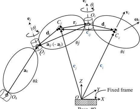
The kinematic constraints in terms of the velocities of two neighbouring links, say, #i and #j, coupled by a revolute joint, as shown in Fig. 2, are given by

ωi=ωj+θ˙iei (3a)

vi=vj+ωj×rj+ωi×di (3b)

whereωjand vjare the angular velocity and velocity of the

mass of link j, i.e., Cj, respectively. Similarly,ωiand viare

defined for the neighbouring link i, whereas ˙θiis the

joint-rate of the i-th joint. The above six scalar equations can be

33 1

Figure 1. A robot manipulator 2

3

4

5

Figure 2: A coupled link system 6

7

ωi

Oj

Cj

aij (- aj)

dj

rj

Oi vi

#j

#i

ej

ei

X Z

Y Fixed frame

O

j

i

Ok

#k

d_i

C_i

c_i c_j

c_ij

Base, #0

ak

#1

#2

2

1 3

Composite Body i

#i

#n n i+1

End-effector

Base, #0

Figure 2.A coupled link system.

written in a compact form as

ti=Bi jtj+piθ˙i (4)

where Bi jis the 6×6 matrix and piis the 6-dimensional

vec-tor which are given by

Bi j≡

"

1 O

ci j×1 1

#

and pi≡

" ei

ei×di

#

(5)

Here, ci jis the 3-dimensional position vector from Cito Cj

given by ci j≡ −di−rj, and ci j×1 is the cross-product tensor

associated with vector ci j. It is defined similar toωi×1 of

Eq. (2). Moreover, ei is the unit vector parallel to the axis

of rotation of the i-th revolute joint. Interestingly, matrix Bi j

and vector pihave the following interpretations:

– If links #i and # j are rigidly attached, Bi j propagates

twist or velocities of # j to #i. Hence, Bi j is termed in

Saha (1999a) as the twist-propagation matrix, which satisfies

Bi jBjk=Bik and Bii=1 (6)

– On the other hand the vector pi takes into account the

motion of the i-th joint. Hence, vector piis termed as the

joint-rate-propagation vector. The vector pi in Eq. (5)

is defined for a revolute joint. For a prismatic joint, it is given by

p_i≡ "

0

ei

#

(7)

Equation (4) can be written for i=1, ..., n, as

S. K. Saha et al.: Evolution of the DeNOC-based dynamic modelling 5 where 1 is the 6n×6n identity matrix, and the 6n×6n matrix

B has the following representation:

B=

                

O O · · · O

B21 O · · · O

..

. ... ... ...

O · · · Bn,n−1 O                 

(8b)

It is now simple matter to invert the 6n×6n matrix, (1−B),

and hence, Eq. (8a) can be rewritten as

t=N ˙θ, where N≡NlNd (9a)

In Eq. (9a), the matrix N is the 6n×n Natural Orthogo-nal Complement (NOC) matrix, as introduced by Angeles and Lee (1988), whereas Nland Nd are the decoupled form of the NOC or the DeNOC matrices proposed first time in Saha (1995). The 6n×6n matrix Nland the 6n×n matrix Nd are given by

Nl=                 

1 O · · · O

B21 1 · · · O

..

. ... ... ...

Bn1 Bn2 · · · 1

                

and

Nd=                 

p₁ 0 · · · 0 0 p₂ · · · 0

..

. ... ... ...

0 0 · · · p_n                 

(9b)

Note that in Eq. (9b), Nl is a lower block-triangular matrix, whereas Ndis a block-diagonal matrix, as indicated through their subscripts “l” and “d”, respectively. Moreover, O and 0 are the 6×6 matrix of zeros and the 6-dimensional vector of zeros, respectively. The n-dimensional vector ˙θis defined as

˙

θ≡hθ1˙ ,· · ·,θ˙n

iT

(10)

which contains the joint-rates of all the joints in the serial-chain system shown in Fig. 1.

2.3 Unconstrained Newton-Euler (NE) equations The unconstrained or uncoupled Newton-Euler (NE) equa-tions of motion for the i-th rigid-link (Saha, 1999a) can be written from its free-body diagram, Fig. 3, as

Iiω˙i+ωi×Iiωi=ni (11a)

mi˙vi=fi (11b)

where ˙ωiand ˙viare the angular acceleration and acceleration

of the mass center Ci, respectively. Moreover, Iiis the 3×3

inertia tensor of i-th link about its mass center Ci, and miis its

mass. Other variables were defined after Eq. (1). The above six scalar equations can be put in a compact form as

34

1

Figure 3. Free-body diagram of the ith link

2

3

4

Figure 4. The Stanford arm

5

ω

O

C

a

d

r

O

v

#

i

X

Z

Y

Inertial frame

O

f

n

c

Revolute

Joint 1

Revolute

Joint 2

Prismatic

Joint 3

Revolute

Joint 4

Revolute

Joint 5

Revolute

Joint 6

Gravity

Figure 3.Free-body diagram of the i-th link.

Mi˙ti+WiMiti=wi (12)

where ti, wiand Wi, Mi are defined in Eqs. (1) and (2),

re-spectively. Moreover, ˙tiis the time derivative of the twist ti

of the i-th link. For the whole system of n rigid links, the 6n scalar equations (for i=1, ..., n, where n is the number of moving rigid links in the serial chain system) can be written as

M ˙t+WMt=w (13)

In Eq. (13), ˙t is the time derivative of the generalized twist, t. Moreover, M and W are the 6n×6n generalized mass matrix and generalized matrix of angular velocities, respectively, i.e.,

M≡diag.[M1,· · ·,Mn] and W≡diag.[W1,· · ·,Wn] (14)

Moreover, w and t are the 6n-dimensional vectors of gener-alized wrench and twist, respectively. They are defined as

w≡hwT₁,· · ·,wT_niT and t≡htT₁,· · ·,tT_niT (15)

2.4 Constrained equations using the DeNOC matrices The kinematic constraints in velocities, i.e., Eq. (9a), then can be incorporated into the unconstrained NE equations of motion, Eq. (13). This is done by pre-multiplying NT _with

the 6n unconstrained NE equations of motions of Eq. (13), i.e.,

NTM ˙t+WMt=NTwE+wC (16)

not do any work, NT_wC_{vanishes (Angeles and Lee, 1988).} Hence, NT_wC_{=0. Substituting the expression of t from} Eq. (9a) and its time derivative, ˙t=NT_{θ¨+N˙˙θinto Eq. (16),}

one can get the n independent scalar dynamic equations of motion, namely,

I ¨θ+C ˙θ=τ (17)

where, I≡NT_{MN: the n×n generalized inertia matrix}

(GIM); C≡NT_{(MN+WMN): the n×n matrix of}

convec-tive inertia terms (MCI); andτ≡NTwE: the n-dimensional vector of generalized forces of driving, and those resulting from gravity, dissipation, and other external forces like foot-ground interaction of a walking robot, etc., if any.

2.5 Analytical expression of the GIM

The analytical expression of the generalized inertia matrix (GIM) appearing in Eq. (17) plays an important role in simplifying, mainly, the forward dynamics agorithm (Saha, 1999a, 2003). In this section, the GIM I is derived using the expressions of the DeNOC matrices (Saha, 1995, 1997, 1999a, b, 2003). Substituting the expressions of the DeNOC matrices given by Eq. (9b) into the expression of the GIM appearing after Eq. (17), one gets

I=NT_dMN˜ d, where ˜M≡NTlMNl (18)

The 6n×6n symmetric matrix ˜M can be written as

˜

M≡

                 

˜

M1 BT₂₁M˜2 · · · BT_n1M˜n ˜

M2B21 M˜2 · · · BT_n2M˜n ..

. ... ... ...

˜

MnBn1 M˜nBn2 · · · M˜n

                 

(19)

where the 6×6 matrix, ˜Mi, for i=1,· · ·, n, can be obtained

recursively, i.e.,

˜

Mi=Mi+BTi₊1,iM˜i₊1Bi₊1,i (20)

in which ˜Mi+1≡O, because there is no (n+1)st link in the serial-chain. Hence, ˜Mn≡Mn. The matrix, ˜Mi, is interpreted

as the mass matrix of the Composite Body, i, that consists of rigidly connected links #i, ..., #n, as indicated in Fig. 1. Finally, the n×n GIM I can be expressed as

I≡

           

i11 sym

.. . ... in1 · · · inn

           

, where ii j≡pTiM˜iBi jpj (21)

for i=1, ..., n; j=1, ..., i. The term ii jis a scalar and “sym”

denotes symmetric elements of the GIM I.

2.6 Recursive inverse dynamics algorithm

The inverse dynamics of a serial-chain system is defined as the process of determining the joint forces/torques when the joint motions of the system are known. The inverse dynamics algorithm calculates the joint torque,τi, for i=1, ..., n, in two

recursive steps, namely, forward and backward recursions. They are given below.

2.6.1 Step 1: forward recursion

First, the 6-dimensional twist and twist-rate vectors of each link, i.e., tiand ˙ti, respectively, are calculated, for i=1, ..., n,

using the following relations:

ti=Bi,i−1ti−1+piθ˙i (22) ˙ti=Bi,i−1˙ti−1+B˙i,i−1ti−1+piθ¨i+˙piθ˙i (23)

wi=Mi˙ti+WiMiti (24)

In the above equations, t0=0 and ˙t0=0, as link #0 is fixed without any motion.

2.6.2 Step 2: backward recursion

The 6-dimensional vector, ˜wi, and the scalar,τi, for i=n, ...,

1, are calculated using the following relations:

˜

wi=BTi₊1,iw˜i₊1, and τi=pTiw˜i (25)

where for i=n, ˜wn+1=0, as there is no (n+1)st link in the system. Hence, ˜wn=wn. The effect of gravity can also be

taken into account by providing negative acceleration due to gravity, g, to the twist-rate of the first link as an additional term (Kane and Levinson, 1983), i.e.,

˙t1=p1θ1¨ +˙p1θ1˙ +ρ, where ρ≡ h

0T,−gTi (26)

Note that Eqs. (22)–(26) were reported in Saha (1999a) with different notations, which actually have the same interpreta-tions as given above, i.e., twist (ti), twist-rate ( ˙ti), wrench

of composite body ( ˜wi), etc. Based on the above mentioned

S. K. Saha et al.: Evolution of the DeNOC-based dynamic modelling 7 2.7 Recursive forward dynamics algorithm

Forward dynamics of a serial-chain system is defined as the process of determining the joint accelerations when the joint-actuator torques/forces of the system are known. In order to compute the joint accelerations ¨θrecursively, the GIM, I of Eq. (17), is decomposed as I≡UDUT (Saha, 1995, 1997, 1999b) based on the Reverse Gaussian Elimination (RGE) method, where U and D are upper triangular and diagonal matrices, respectively. The UDUT decomposition results in an efficient order n, i.e., O(n), computational algorithm in contrast to O(n3_{) computations required by the Cholesky} de-composition of the GIM (Strang, 1998).

For the development of recursive O(n) forward dynam-ics algorithm, the constrained dynamdynam-ics equations of motion, Eq. (17), are rewritten as

UDUTθ¨=ϕ (27)

whereϕ≡τ−C ˙θ. Then, three recursive steps are used to cal-culate the joint accelerations, which are given below.

2.7.1 Step 1

Solution for ˆτ, where ˆτ≡DUTθ¨≡U−1ϕ. It is found as fol-lows: For i=n−1, ..., 1, calculate

ˆ

τi=ϕi−pTiηi,i+1 (28) whereη_i,i+1is the 6-dimensional vector obtained recursively as

ηi,i₊1≡BTi₊1,iηi₊1 and ηi+1≡τˆi₊1ψi+1+ηi+1,i+2 (29) in which η_n,n+1=0, and the 6-dimensional vector ψi₊1 is evaluated using the following relations:

ψ_i= ψˆi

ˆ mi

, where ˆψi≡Mˆipi and ˆmi≡pTiψˆi (30)

In Eq. (30), the 6×6 matrix, ˆMiis obtained recursively as ˆ

Mi=Mi+BTi+1,iMi+1Bi+1,i,

where Mi+1≡Mˆi+1−ψˆi+1ψTi+1and ˆMn=Mn (31)

The 6×6 symmetric matrix ˆMiis the mass matrix of Artic-ulated Body, i, defined as the links #i, ..., #n, coupled by the joints i+1, ..., n. This is in contrast to the definition of the Composite Body, i, given after Eq. (20), where the links are rigidly connected, i.e., the joints are locked. Note that the mass matrix of the i-th Articulate Body ˆMiis nothing but the

Articulated-Body-Inertia (ABI) of Featherstone (1987).

2.7.2 Step 2

Solution for ˜τ, where, ˜τ≡UT_θ¨≡D−1_{τˆ. It is found as follows:} for i=1, ..., n,

˜ τi=

ˆ τi

ˆ mi

(32)

34 1

Figure 3. Free-body diagram of the ith link 2

3

4

Figure 4. The Stanford arm 5

ωi

Oi

Ci ai

di

ri

Oi+1

vi

# i

X Z

Y

Inertial frame

O

fi ni

c

i

Revolute Joint 1 Revolute

Joint 2

Prismatic Joint 3

Revolute Joint 4

Revolute Joint 5

Revolute Joint 6 Gravity

Figure 4.The Stanford arm.

2.7.3 Step 3

Solution for ¨θ, where, ¨θ≡U−Tτ˜. It is found as follows: For i=2, ..., n,

¨

θi=τ˜i−ψTiµi,i−1 (33)

whereµ_i,i−1≡Bi,i−1µi−1,µi−1≡pi−1θ¨i−1+µi−1,i−2, and for i= 1,µ₁₀≡0.

Based on the above mentioned forward dynamics algo-rithm, another C++program RFDSIM (Recursive Forward Dynamic and Simulation of Industrial Manipulators) was written which was reported in Saha (1999a). A similar al-gorithm was rewritten in Visual C# and implemented in the “FDyn” module of RoboAnalyzer software (Rajeevlochana et al., 2012; http://www.roboanalyzer.com) with which one can see animation of the systems under study. The numerical integrator used in RoboAnalyzer for the simulation purposes is based on the Runge-Kutta 4th order method (Bathe and Wilson, 1976).

2.8 Numerical example: a 6-DOF Stanford arm

The dynamic analyses of the 6-link 6-DOF serial-chain sys-tem with both revolute and prismatic joints, namely, the Stan-ford arm as shown in Fig. 4, were carried out using RoboAn-alyzer. The Denavit and Hartenberg (DH) paramters, which were proposed by Denavit and Hartenberg (1955), and the mass and inertia propoerties are taken from Saha (1999a) as per the notations explained there and in Saha (2008). The numerical values are not reproduced here since the focus of this paper is to review the DeNOC-based formulations and their applicability. However, the joint torques (Joints 1–2, 4– 6) and force (Joint 3) obtained from the “IDyn” module of RoboAnalyzer software for the following joint input motions are plotted in Fig. 5:

θi=θi(0)+

θi(T )−θi(0) T

"

t− T

2πsin 2π

T t

!#

35 1

Figure 5. Joint torques (1-2, 4-6) and force (3) for the Stanford arm 2

0 0.5

0 0.2 0.4 0.6 0.8

time(s) 1

(

d

e

g

)

0 0.5

-100 -80 -60 -40

time(s) 2

(

d

e

g

)

0 0.5

600 800 1000 1200

time(s)

b3

(

m

m

)

0 0.5

-6 -4 -2 0 2

time(s) 4

(

d

e

g

)

0 0.5

179 179.5 180

time(s) 5

(

d

e

g

)

0 0.5

180 182 184 186

time(s) 6

(

d

e

g

)

3

4

Figure 6. Simulated joint motions for the free-fall of the Stanford arm 5

6

7

b3

Figure 5.Joint torques (1–2, 4–6) and force (3) for the Stanford

arm.

35 1

Figure 5. Joint torques (1-2, 4-6) and force (3) for the Stanford arm 2

0 0.5

0 0.2 0.4 0.6 0.8

time(s)

1

(

d

e

g

)

0 0.5

-100 -80 -60 -40

time(s)

2

(

d

e

g

)

0 0.5

600 800 1000 1200

time(s) b3

(

m

m

)

0 0.5

-6 -4 -2 0 2

time(s)

4

(

d

e

g

)

0 0.5

179 179.5 180

time(s)

5

(

d

e

g

)

0 0.5

180 182 184 186

time(s)

6

(

d

e

g

)

3

4

Figure 6. Simulated joint motions for the free-fall of the Stanford arm 5

6

7

b3

Figure 6.Simulated joint motions for the free-fall of the Stanford

arm.

b3=b3(0)+

b3(T )−b3(0)

T

"

t− T

2πsin 2π

T t

!#

(35)

whereθi(0)=0, for i=1–2, 4–6 and b3(0)=0 are the vari-able DH parameters (Saha, 2008) or the joint varivari-ables at time T=0, whereas the total time of motion is, T=10 s. Gravity was acting in the negative Z1-direction. The variable,

τi, for i=1–2, 4–6, and f3in Fig. 5 are the joint torques and force, respectively. The results were verified with those re-ported in Saha (2008).

The forward dynamics and simulation of the Stanford arm was also performed using “FDyn” module of RoboAnalyzer. The Stanford manipulator was assumed to fall freely under gravity without any external torques and force at the actu-ating joints. The initial positions were taken same as in the inverse dynamics analysis given after Eq. (35). The results are plotted in Fig. 6, where the variations of the joint mo-tions with respect to time are shown. The results were also verified with those reported in Saha (2008).

36

0 Base

A link or body

Figure 7. A tree-type system

0

M1

Base

Ms

Mβ

A kinematic module

M0

Mi

Figure 8. The multi-modular tree-type system

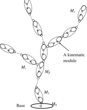
Figure 7.A tree-type system.

3 Tree-type systems

A tree-type system has a set of links connected by kinematic pairs, typically, a revolute or a prismatic joint, as shown in Fig. 7. Other type of joints, say, a universal or spherical, and a cylindrical, can be modelled as a combination of two or three intersecting revolute joints, and a pair of revolute-prismatic joints, respectively, as mentioned in the beginning of Sect. 2.1. Based on the modelling of serial-chain systems, Shah et al. (2011, 2013) extended the methodology to model a tree-type system. For this, the tree-type system was as-sumed to be a combination of several serial-chain systems called “kinematic modules”. Consequently, multi-modular recursive algorithms for the tree-type systems were presented against “full-body-level” recursive dynamics algorithms of Featherstone (1987) and Rodriguez (1992). Each “module” of the tree-type architecture was defined as a set of serially connected links emerges from the last link of its parent mod-ule. For example, as indicated in Fig. 8, the parent module of Miis module Mβ.

For the analyses purposes, the tree-type system was first kinematically modularized before its kinematic constraints were derived. The modules are denoted with M0, M1, M2, etc., where a child module bears a number higher than its parent module. Moreover, the links inside any module, say, Mi, are denoted as #1i, ..., #ki, ..., #ηi, where the

super-script i signifies the module number. Considering the tree-type system, there are s number of modules in the system, and there areηinumber of links in the i-th module. The to-tal number of links in the whole system is then obtained by

n=

s

P

i

ηi_{. The kinematic constraints were next derived at the}

S. K. Saha et al.: Evolution of the DeNOC-based dynamic modelling 9

36 0

Base

A link or body

Figure 7. A tree-type system

0

M1

Base

Ms

Mβ

A kinematic module

M0

Mi

Figure 8. The multi-modular tree-type system

Figure 8.The multi-modular tree-type system.

and inter-modular (between the modules) recursions, as pre-sented in Fig. 9.

3.1 Intra-modular kinematic constraints

Intra-modular kinematic constraints are effectively the veloc-ity constraints between the links of a serial-chain system de-rived in Eqs. (3–10). Here, however, a little modification is proposed in the definition of each link’s linear velocity vi. In

contrast to the definition of the velocity of the mass center of the i-th link, Ci, as viof Eq. (1), it is defined in this section as

the velocity of point Oiwhere the i-th joint couples the j-th

link with the i-th one, as indicated in Fig. 2. Such definition of viin twist expression of Eq. (1) was necessitated mainly to

take care of the branching issue of the serial-modules in the tree-type system, as shown in Fig. 8. The velocity of the i-th link defined here with respect to Oi (sometimes referred to

as the origin of the i-th link). It is actually the velocity of the previous link at its connection point, namely, the last link of the parent module where the first link of the child module is coupled. Hence, where branching occurs no additional com-putations are required for the calculation of the velocity of the first link belonging to the child module. This was not the case with the definition of the velocity of the i-th link with respect to its mass center Ci in which additional

computa-tions would be required to calculate the velocity of the mass center Ci from the origin Oi. Moreover, as the main

objec-tive of dynamic analyses is to calculate either joint torques or joint motions, selection of Oias a reference point, instead

of the Ci, can lead to efficient recursive inverse and forward

dynamics algorithms, as shown by Shah et al. (2011, 2013). In fact, for the serial-chain systems considered in Sect. 2, the same definition with respect to Oicould have been adopted.

This was done with the “IDyn” and “FDyn” modules of the RoboAnalyzer software. In Sect. 2, however, it was shown

how the simplest form of the NE equations of motion given by Eq. (1) can be used with the definition of the DeNOC ma-trices, as demonstrated in the original work of Saha (1995, 1997, 1999a, b, 2003).

Now, with the new definitions of vi with respect to Oi,

Eq. (4) is rewritten as

ti=Ai jtj+piθ˙i (36a)

where tiand tjare the 6-dimensional twist vectors defined in

Eq. (1) but with respect to (w.r.t.) the new definition of vi, i.e.,

w.r.t. point Oi. Accordingly, the 6×6 matrix Ai j is the new

twist-propagation matrix. A different notation is used here to distinguish it from Bi jwhich was defined after Eq. (4) w.r.t.

the definition of the velocity of Ci. The 6×6 matrix Ai j, and

the 6-dimensional joint-rate-propagation vector, pi, are given

by

Ai j=

"

1 O

ai j×1 1

#

, and

p_i= "

ei 0

#

for revolute; p_i=

"

0

ei

#

for prismatic (36b)

where the 3-dimensional vector ai jis shown in Fig. 2. Notice

the change in the expression of piin Eq. (36b) in comparison

to the same in Eq. (5) where viwas defined w.r.t. Ci. For

seri-ally connected rigid links in the i-th serial-chain module, one can write the expression for the generalized twist, ti, similar

to Eq. (9a), as

ti=Ni ˙

θi, where Ni≡[NlNd]i (37)

In Eq. (37), the 6ηi_{-dimensional generalized twist vector t} i

and theηi_{-dimensional generalized joint-rates vector θ}˙

i are

defined as follows:

ti≡

                        

t1

.. .

tk .. .

tη

                        

i

and θ˙i≡

                         

˙

θ1

.. .

˙

θk .. .

˙

θη

                         

i

(38)

where a bar (“−”) over an entity in Eqs. (37) and (38) sig-nifies that the quantity is related to a module and the super-script, i, outside the brackets identifies the module. As a con-sequence, the generic notation tk (or tki) in Eq. (38) is the 6-dimensional twist vector for the kth_{link in the i-th module.} The 6ηi_×6ηi_{and 6η}i_×ηi_{DeNOC matrices for the serial-chain}

a. Inverse dynamics b. Forward dynamics

Figure 9. Recursive dynamics algorithms (Shah, 2011; Shah et al., 2013)

( ) ( ) , ( ) N w

w w A w

T i i i

T i i i i i

,

, ,

t A t N θ

t A t +A t +N θ N θ

w =M t Ω M E t

i

i i

i i i i

i i i i i i i

i i i i i i i i = 1:s

i = s:1

Joint torques ( ) τi

Joint motions ( , , )θ θ θi i i , inertia

parameters (Mi), twist and motion propagations (Ai, and Ni)

Fo

rwar

d

rec

u

rs

io

n

B

ac

k

war

d

rec

u

rs

io

n

1

1

,

( ) ( ) ,, (( )) , , ( )

( ) ( ) , ( )

ˆ ˆ _; ˆ ˆ _; ˆ ˆ

ˆ ˆ ˆ

ˆ

ˆ ˆ _; ˆ

ˆ ˆ ˆ

i i i T

i i i i i i T

i i i i

i i i T

i i i i i i i i i T

i i ii ii i i i i T

i i i i i

Ψ M N I N Ψ Ψ Ψ I

φ φ N η

φ I φ

M M Ψ Ψ η Ψ φ η

M M A M A

η η A η

,

, ,

*

i

i i

i i i i

i i i i i

i i i i i i i

t A t N θ

t A t +A t +N θ

w =M t Ω M E t

i = 1:s

i = s:1

, ( )

( ) ( ) ( )

( )

,

i i

i i i i

T i i i i

μ A N q μ

θ φ Ψ μ

i = 1:s

Independent accelerations θ

Joint torques( )τi , inertia parameters(Mi), twist

and motion propagations (A i j_, and Ni), and

initial conditions θi, and θi

Fo

rwar

d

rec

u

rs

io

n

B

ac

k

war

d

rec

u

rs

io

n

Fo

rwar

d

rec

u

rs

io

n

Figure 9.Recursive dynamics algorithms (Shah, 2011; Shah et al., 2013).

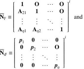
Nli≡                 

1 O · · · O

A21 1 · · · O

..

. ... ... ...

Aη1 Aη2 · · · 1                 

i

and

Ndi≡                 

p₁ 0 · · · 0 0 p₂ · · · O

..

. ... ... ...

0 0 · · · p_η                 

i

(39)

3.2 Inter-modular kinematic constraints

Having obtained the intra-modular kinematic constraints in the velocity-level, it is now possible to derive the inter-modular kinematic (velocity) constraints, i.e., between two neighbouring serial-chain modules. In a way, each module has been treated similar to a link in a serial-chain module presented in Sect. 2 or Sect. 3.1. For this, module Mβis

con-sidered as the parent of module Mi, as shown in Fig. 8. This

is similar to link j of Fig. 2 which is the parent of link i. The 6ηi_{-dimensional generalized twist t}

i is then obtained from

the 6ηβ-dimensional generalized twist tβas

ti=Ai,βtβ+Ni ˙

θi (40)

where Ai,β is the 6ηi×6ηβ module-twist-propagation matrix which propagates the generalized twist of the parent module (β) to the child module (i) and Niis the 6ηi×ηi

module-joint-rate propagation matrix, which are given by

Ai,β≡

           

O · · · O A1i_,ηβ

..

. ... ... ...

O · · · O Aηi_,ηβ            

S. K. Saha et al.: Evolution of the DeNOC-based dynamic modelling 11 and

Ni=[NlNd]i≡                 

p1 0 · · · 0

A21p1 p2 · · · 0

..

. ... ... ...

Aη1p1 Aη2p2 · · · pη                  i (41b)

The vectors ti and ˙

θi are defined in Eq. (38). Next,

the 6dimensional generalized twist vector t, and the n-dimensional generalized joint-rate vector ˙θ, for the whole tree-type system which comprises of s modules and n links are defined as

t≡h _tT

0 t

T

1 · · · t

T

i · · · t T s iT and ˙ θ≡ ˙ θT 0 ˙ θT

1 · · ·

˙

θT i · · ·

˙

θT s

T

(42)

where t0 and

˙

θ0 correspond to the base module M0 which may not be fixed. For example, in the case of a spacecraft carrying a manipulator, the spacecraft floats with motion of 6-degrees-of-freedom (DOF). For the analysis purposes, its motion need to be specified for further motion analyses of other modules, e.g., the manipulator of the above system.

Upon substitution of the expressions of Nifrom Eq. (41b),

for i=1,..., s, in Eq. (40), and manipulating the expres-sions like Eqs. (8)–(9), one obtains the expression of the 6n-dimensioanl generalized twist t for the whole tree-type sys-tem as

t=NlNdθ˙ (43)

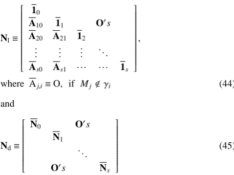
in which, Nland Ndare the 6(n+1)×6(n+1) and 6(n+1)× (n+n0) matrices, respectively, as the tree-type system was assumed to have module M0with one-link with n0DOF. Ma-trices Nland Ndfor the tree-type system are given by

Nl≡                          10

A10 11 O0s

A20 A21 12

..

. ... ... ...

As0 As1 · · · 1s

                         ,

where Aj,i≡O, if Mj<γi (44)

and

Nd≡                   

N0 O0s

N1

...

O0_{s N}

s                    (45)

In Eq. (44), 1i is the 6ηi×6ηi identity matrix, whereas γi

stands for the array of all modules including module Miand

outward to it, as shown within dashed line of Fig. 10. The

38

M

i

j

Figure 10. Definition of i

3 4 5 Spherical joints at hips Revote joints at knees Universal joints at ankles 0 #11 #2 31 11 21 #31 M1 #12 #22 #32 12 22 32 M2 M0

Y (Sidewise)

Z (Vertical)

X (Forward)

(a) Biped architecture (b) Modules of the biped

Figure 11. A 7-link spatial biped

Trunk

Serial chain

inside ith module

Figure 10.Definition ofγi.

matrices Nl and Nd are the desired Decoupled Natural Or-thogonal Compliment (DeNOC) matrices for the whole tree-type system at hand. Note here that the matrices, Nland Nd of Eq. (9b), and Nliand N_di of Eq. (39), are the special cases of the DeNOC matrices derived in Eqs. (44) and (45), where each module has only one link without any branching.

3.3 Newton-Euler (NE) equations for tree-type systems In contrast to the expressions for the Newton-Euler (NE) equations of the i-th link given by Eq. (11) or (12), a de-viation in their expressions will be observed. This is due to the modified definition of the velocity of the i-th link, i.e., vi,

with respect to point Oi. This was mentioned in Sect. 3.1. The

NE equations of motion of the k-th link (as the letter “i” will be used to denote module) of the i-th module with respect to point Okcan be expressed as (Shah et al., 2011, 2013)

Ikω˙k+mkdk×˙vk+ωk×Ikωk=nk (46a)

mkvk−mkdk×ω˙k−ωk×(mkdk×ωk)= fk (46b)

Combining Eqs. (46a)–(46b), one can obtain an expression equivalent to Eq. (12) as

Mk˙tk+ ΩkMkEktk=wk (47a)

where the 6×6 matrices Mk,Ωk, and Ekare defined as

Mk≡

"

Ik mkdk×1

−mkdk×1 mk1

#

, Ωk≡

" _ω

k×1 O

O ωk×1

#

,

and Ek≡

"

1 O

O O

#

(47b)

Note in Eq. (47b), that Ikis the 3×3 mass moment of inertia

tensor of the k-th link about Ok. Combining Eq. (47a) for all ηi _{links of the i-th module and for all s modules, one can}

write a compact expression equivalent to Eq. (13) as (Shah et al., 2011, 2013)

12 S. K. Saha et al.: Evolution of the DeNOC-based dynamic modelling

38

M

i

Detail inside

the module

j

1

2

Figure 10. Definition of

i

3

4

5

Spherical joints at hips

Revote joints at knees

Universal joints at ankles

0

#11

#2

31

11

21

#31

M1

#12

#22

#32

12

22

32

M2

M0

Y (Sidewise) Z (Vertical)

X (Forward)

(a) Biped architecture

(b) Modules of the biped

Figure 11. A 7-link spatial biped

Serial chain

inside

i

th module

Figure 11.A 7-link spatial biped.

where matrices M,Ω, and E are the 6(n+1)×6(n+1) block-diagonal matrices defined similar to Eq. (14). For details, readers are referred to the Ph.D. thesis of Shah (2011) or the book by Shah et al. (2013).

3.4 Constrained equations for tree-type systems using the DeNOC matrices

The constrained equations of motion for the tree-type sys-tems are derived in this subsection in a similar manner to that of the serial-chain system of Sect. 2, i.e., pre-multiply NT_dNT_l

of Eq. (43) to the unconstrained NE equations given by Eq. (48) to obtain a set of constrained independent equations of motion by eliminating the constraint wrenches. These con-strained equations are also referred to as the Euler-Lagrange equations of motion of the tree-type system at hand. They are given by

I ¨θ+C ˙θ=τ (49)

where I is generalized inertia matrix (GIM), C is the matrix of convective inertia terms (MCI), andτis the vector of gen-eralized driving forces, and due to gravity, dissipation, exter-nal forces, etc., which have expressions similar to those after Eq. (17).

Note that the expression of Eq. (49) is same as Eq. (17) but the sizes of the corresponding matrices and vectors are different because they represent two different architectures of the multibody systems. Based on Eq. (49), recursive inverse and forward dynamics algorithms for tree-type systems were developed by Shah (2011) and implemented in a software called ReDySim (Recursieve Dynamics Simulator) (Shah et al., 2012c). ReDySim was written in MATLAB environment and available free from http://www.redysim.co.nr.

1 2

Figure 12 Designed trajectories of the trunk’s center of mass (COM) and ankle (Shah, 2011; 3

Shah et al., 2013) 4

5

0 0.5

-0.2 0 0.2

x0

time (sec)

0 0.5

0 0.01 0.02

y0

time (sec)

0 0.5

-1 0 1 2

z0

time (sec)

0 0.5

-0.5 0 0.5

xa

time (sec)

0 0.5

-0.06 -0.04 -0.02 0

ya

time (sec)

0 0.5

-0.1 0 0.1

za

time (sec) (a) Trunk‘s COM

0 0.5

-0.2 0 0.2

x0

time (sec)

0 0.5

0 0.01 0.02

y0

time (sec)

0 0.5

-1 0 1 2

z0

time (sec)

0 0.5

-0.5 0 0.5

xa

time (sec)

0 0.5

-0.06 -0.04 -0.02 0

ya

time (sec)

0 0.5

-0.1 0 0.1

za

time (sec)

(b) Ankle of the swing foot

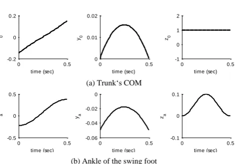
Figure 12. Designed trajectories of the trunk’s center of mass

(COM) and ankle (Shah, 2011; Shah et al., 2013).

3.5 Numerical example: a spatial biped

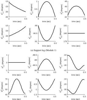
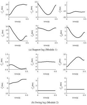
In order to illustrate the recursive dynamics algorithms pre-sented in this section, ReDySim was used to analyze a spatial biped shown in Fig. 11. The model parameters were taken from Shah (2011) which will appear in the book by Shah et al. (2013) also. They are not reproduced here due to the reasons cited in Sect. 2.8. However, the designed input mo-tions of the trunk’s centre-of-mass (COM) and ankle for sta-ble walking (Shah, 2011) are shown in Figs. 12 and 13, re-spectively. Based on the inputs of Figs. 12 and 13, the inverse dynamics results were obtained which are shown in Fig. 14.

Forced simulation was performed next, as reported in Shah (2011), where the motion of the biped was studied un-der the application of joint torques calculated above, i.e.,

S. K. Saha et al.: Evolution of the DeNOC-based dynamic modelling 13

40 1

2

0 0.5

-40 -30 -20 -10

1,1

1

(

d

e

g

re

e

)

time (sec)

0 0.5

0 0.5 1

1,2

1

(

d

e

g

re

e

)

time (sec)

0 0.5

42 44 46 48

2

1 (

d

e

g

re

e

)

time (sec)

0 0.5

-40 -30 -20 -10

time (sec)

3,1

1

(

d

e

g

re

e

)

0 0.5

-91 -90.5 -90

3,2

1

(

d

e

g

re

e

)

time (sec)

0 0.5

179 180 181

time (sec)

3,3

1

(

d

e

g

re

e

)

(a) Support leg (Module 1)

0 0.5

-1 0 1

1,1

2

(

d

e

g

re

e

)

time (sec)

0 0.5

-90 -89.5 -89 -88.5

time (sec)

1,2

2

(

d

e

g

re

e

)

0 0.5

-40 -30 -20 -10

1,3

2

(

d

e

g

re

e

)

time (sec)

0 0.5

40 50 60 70

2 2 (

d

e

g

re

e

)

time (sec)

0 0.5

-1.5 -1 -0.5 0

3,1

2

(

d

e

g

re

e

)

time (sec)

0 0.5

-40 -30 -20 -10

3,2

2

(

d

e

g

re

e

)

time (sec)

(b) Swing leg (Module 2)

Figure 13. Joint trajectories of the biped obtained from the trajectories of trunk and ankle (Shah, 2011; Shah et al., 2013)

Figure 13.Joint trajectories of the biped obtained from the trajectories of trunk and ankle (Shah, 2011; Shah et al., 2013).

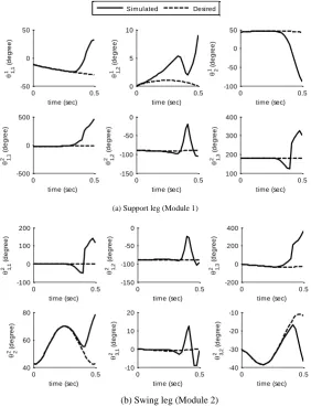
those shown in Fig. 14. The joint motions were calculated using the forward dynamics module of ReDySim. The plots for the simulated joint angles are shown in Fig. 15, along with the desired one. It can be seen that the simulated joint angles match with the desired joint angles up to 0.1 s, i.e., until 0.1 s movement of the biped. After this, the system behaves unex-pectedly as evident from the divergent plots of the simulated angles in Fig. 15a. The deviation in the simulated angles is mainly attributed to what is known as zero eigen-value ef-fect (Saha and Schiehlen, 2001). The physical system may also not behave as expected due to disturbances caused by unmodelled parameters like friction, backlash, etc., and non-exact geometrical and inertia parameters. Hence, a control scheme must be considered, as this forms a part and parcel of achieving proper walking. These aspects were explained in detail in Shah (2011) and Shah et al. (2013), and not elab-orated further due to space limitation of the paper.

Note several advantages of the concept of the kinematic modules in the dynamics modelling of tree-type systems con-sisting of serially connected links (Shah, 2011; Shah et al., 2013), which are as follows:

– Extension of the body-to-body velocity transformation

relationship to module-to-module velocity transforma-tion relatransforma-tionship.

– Compact representation of the system’s kinematic and

dynamic models.

– Uniform development of the inverse and forward

dy-namics algorithms with inter- and intra-modular recur-sions.

– Module-level analytical expressions of the matrices and

vectors appearing in the equations of motion.

– Ease of investigation of any inconsistency in the results

of modules without the need to investigate the whole system.

– Possibility of hybrid recursive-parallel algorithms,

41 1

2

3

0 0.5

-10 0 10

time(s)



1 1,1

(

N

m

)

0 0.5

4 6 8 10

time(s)



1 1,2

(

N

m

)

0 0.5

-20 -10 0

time(s)



1 (2

N

m

)

0 0.5

-5 0 5 10 15

time(s)



1 3,1

(

N

m

)

0 0.5

-4 -2 0 2 4 6

time(s)



1 3,2

(N

m

)

0 0.5

-1 0 1 2

time(s)



1 3,3

(N

m

)

(a) Support leg (Module 1)

0 0.5

-0.5 0 0.5 1 1.5

time(s)



2 1,1

(

N

m

)

0 0.5

-6 -4 -2 0 2 4

time(s)



2 1,2

(

N

m

)

0 0.5

-20 -10 0 10

time(s)



2 1,3

(N

m

)

0 0.5

-10 -5 0 5

time(s)



2 (2

N

m

)

0 0.5

0 2 4

time(s)



2 2,1

(N

m

)

0 0.5

-2 0 2 4 6

time(s)



2 2,2

(

N

m

)

(b) Swing leg (Module 2)

Figure 14. Torques at different joints of the biped (Shah, 2011; Shah et al., 2013)

Figure 14.Torques at different joints of the biped (Shah, 2011; Shah et al., 2013).

4 Closed-loop systems

The DeNOC-based dynamic modelling of serial-chain and tree-type open-loop systems presented in Sects. 2 and 3, respectively, can be extended to closed-loop systems pro-vided one cuts the closed-loops of a system at suitable lo-cations to make it open. Note that, one needs to use suit-able constraint forces at the cut-joints to represent the actual presence of the joints. Such constraint forces are known in the literature as Lagrange multipliers (Chaudhary and Saha, 2007, 2009, and others). The multipliers need to be evalu-ated from the loop-closure constraints before they can be used as external forces to the resulting open-loop systems. In this section, a planar 4-bar mechanism shown in Fig. 16 is considered to illustrate the concept. However, the methodol-ogy is applicable to any general multi closed-loop systems, as shown in Chaudhary and Saha (2007), Shah (2011), and Shah et al. (2013).

Note that to model an open-loop system resulting from a closed-loop system, one needs to re-write Eqs. (13) or (48) as

NT(M ˙t+ΩMEt)=NT(wE+wλ+wC) (50)

where wλis the 6n-dimensional vector of generalized wrench due to Lagrange multipliers acting at the cut joints. For the 4-bar mechanism shown in Fig. 16a, the two cut-open serial-chain subsystems are shown in Fig. 16b. The resulting open-loop tree-type subsystems have one and two links, respec-tively, connected by one and two one-DOF revolute joints. Other terms have same meaning as in Sects. 2 and 3. In Eq. (50), NTwC=0 for the reason given after Eq. (16), but

NTwλ,0. These terms are now the new unknowns to the inverse and forward dynamics problems that need to be eval-uated with the help of loop-closure constraints.

For the closed-loop 1-2-3-4 of the 4-bar mechanism shown in Fig. 16a, one can write

a0+a1=a2+a3 (51)

where 2-dimensional vectors of the planar system, aifor i=

0, 1, 2, 3, represent the relative position vectors of the joints in the 4-bar mechanism, Fig. 16a. Differentiating Eq. (51) with respect to time, one obtains

S. K. Saha et al.: Evolution of the DeNOC-based dynamic modelling 15

42 t 1

2

3

4

0 0.1 0.2 0.3 0.4 0.5 0.6 0.7 0.8 0.9 1

-0.2 0 0.2

time(s) X0

(m

)

0 0.1 0.2 0.3 0.4 0.5 0.6 0.7 0.8 0.9 1

time(s) X0

(m

)

0 0.1 0.2 0.3 0.4 0.5 0.6 0.7 0.8 0.9 1

time(s) X0

(m

)

Actual Designed

Simulated Desired

Simulated Desired

0 0.5

-50 0 50

1,1

1

(

d

e

g

re

e

)

time (sec)

0 0.5

0 5 10

1,2

1

(

d

e

g

re

e

)

time (sec)

0 0.5

-100 -50 0 50

2 1 (

d

e

g

re

e

)

time (sec)

0 0.5

-500 0 500

time (sec) 1,1

2

(

d

e

g

re

e

)

0 0.5

-150 -100 -50 0

1,2

2

(

d

e

g

re

e

)

time (sec)

0 0.5

100 200 300 400

time (sec) 1,3

2

(

d

e

g

re

e

)

(a) Support leg (Module 1)

0 0.5

-100 0 100 200

1,1

2

(

d

e

g

re

e

)

time (sec)

0 0.5

-150 -100 -50 0

time (sec) 1,2

2

(

d

e

g

re

e

)

0 0.5

-200 0 200 400

1,3

2

(

d

e

g

re

e

)

time (sec)

0 0.5

40 60 80

2 2 (

d

e

g

re

e

)

time (sec)

0 0.5

-10 0 10 20

3,1

2

(

d

e

g

re

e

)

time (sec)

0 0.5

-40 -30 -20 -10

3,2

2

(

d

e

g

re

e

)

time (sec)

(b) Swing leg (Module 2)

Figure 15. Simulated joint angles for the biped (Shah, 2011; Shah et al., 2013)

Figure 15.Simulated joint angles for the biped (Shah, 2011; Shah et al., 2013).

and the 2×3 Jacobian matrix for the 4-bar mechanism at hand can be given by

J≡

"

−a1s1−a2s12+a3s123 −a2s