http://www.sciencepublishinggroup.com/j/ijamtp doi: 10.11648/j.ijamtp.20190503.16
ISSN: 2575-5919 (Print); ISSN: 2575-5927 (Online)
Forced Nutation for Rigid Earth Model with Different
Theories
Mohamed Soliman
1, Hadia Hassan Selim
1, *, Inal Adham Hassan
21
Department of Astronomy, National Research Institute of Astronomy and Geophysics, Helwan, Egypt
2
Department of Astronomy and Metrology, Al-Azhar University, Cairo, Egpyt
Email address:
*
Corresponding author
To cite this article:
Mohamed Soliman, Hadia Hassan Selim, Inal Adham Hassan. Forced Nutation for Rigid Earth Model with Different Theories. International Journal of Applied Mathematics and Theoretical Physics. Special Issue: Theory and Applications for Rotational Earth and Space Dynamics. Vol. 5, No. 3, 2019, pp. 85-96. doi: 10.11648/j.ijamtp.20190503.16
Received: August 13, 2019; Accepted: September 10, 2019; Published: September 23, 2019
Abstract:
Where Earth is not strictly rigid body but can responds to any effects that tend to its rotation and shape, we will explain, in the present paper, the goal which is to define the forced nutation for a rigid Earth model using two different theories. We will formulate a first order Hamiltonian of a deformable Earth for its rotational motion around the Sun through the contribution of triaxial symmetry of the Earth. The formulation of the theory will be formed twice times. Firstly, deduce the tidal affect’s forces by Luni - Solar attraction coupling with the Earth’s geopotential force. Secondly, through the formulation, we will neglect the coupling between the different effects (the geopotential Earth force effect and the Luni - Solar attraction force), so, we will find the transform of the Hamiltonian for each force separately. The analytical solution for the formulated Hamiltonian will be derived for the two cases by using perturbation technique of Lie - Hori series. Once can get the analytical solution by getting the generation function, we will derive the nutation series analytically and numerically for each case and conclude over the results.Keywords: Rotation of the Earth, Forced Nutation, Celestial Mechanics
1. Introduction
Because of Earth is responds to any effect to be as a deformable body and not as a strictly rigid, it is possesses some sort of elastic properties [1]. Many papers concerned with the study of a rotation for a deformable Earth through different theories of Earth’s model as the series of papers [2-6] and another series [7-13]. So, its shape changes through the rotational motion about its axis, this change affects on the periodic rotation and its uniformity, which intern affects on its shape, also, the same done due to the tidal effects of Sun and Moon.
The present work is concerned with these affects which have been studied twice times, firstly as a coupling effects of rotational Earth including its geopotential and the tidal effects produced with its motion around the Sun through its orbit including the Moon’s gravitational effects, secondly, we will concern with neglecting the coupling between the
different effects. Short periodic nutation terms will be treated in Hamiltonian form through the contributions of triaxial symmetry of the Earth in each theory and the comparison of results will be done.
2. Canonical Transformation
Andoyer and Euler system’s variables will be obtained through a canonical transformation [2].
In the case of the body assuming rigid, by taking into account its elasticity such as responds to effects produced by its rotation and by other external tidal effects, we taking into account the Andoyer and Euler angles variables.
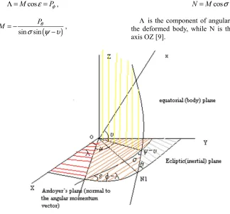
As shown in figure 1, the angles λ, µ and ν are correspond to Andoyer’s variables while ℓm s, ,gm s, and hm s, corresponding Delaunay’s variables for Moon and Sun respectively.
cos
M
ε
PφΛ = = ,
(
)
sin sin
P
M θ
σ ψ υ
= −
− ,
cos
N=M
σ
=Pψ (1)Λ is the component of angular momentum of rotation of the deformed body, while N is the component on the body axis OZ [9].
Figure 1. Euler and Andoyer Angles.
3. The Hamiltonian
The Hamiltonian H describing deformable Earth under tidal effects written as [2-4]
2
r t E r r
H = + + +T T T R +E + +V V (2)
Where
T: is the K. E. for the torque free rigid Earth rotation.
r
T : is the increase in the K. E. due to the rotational deformation.
t
T: The increase in the K. E due to the tidal deformation.
E
R : The contribution from the motion of the ecliptic of
date.
r
E : The elastic strain energy stored by the rotational deformation.
2
V : The potential energy due to motion of the disturbing bodies, with assumed triaxial solid.
r
V : The increase of potential energy due to the effect of these quantities.
Which defined as:
2 2 sin2 cos2 2
2 2
M N N
T
A B c
υ
υ
−
= − +
(3)
2 2 2
2
1 1 1 3
3 sin sin 2 cos cos sin sin 2 sin 2
2 4
r r r r r r r
M M N
T D D
c A B A AB
σ
σ
υ
υ
−σ
υ
υ
= + − +
(4)
(
)
2(
)
2 2 2 2
1 1 1 2
sin 2
t t
N
T D M N P
A B c δ
∗
= − − + +
(
2 2)
(
(
)
2(
)
)
2 2
2 2
1 1 1
2 sin cos 2 sin cos 2
4 M N A B P δ υ P δ α
∗ ∗ ∗
+ − − +
]
2 2 2 2
2 2
2 2
1 1 1 2
( )[( ) (sin ) cos 2 cos 2 (sin )sin 2 sin 2
4 M N A B P
δ
α
ν
ABPδ
α
ν
∗ ∗ ∗ ∗
(
)
(
)
2
1 1
2 2
1 1
sin 2 sin cos sin sin sin cos
M
P P
C σ A δ α ν B α α ν
∗ ∗ ∗
+ +
(5)
1 2
sin
E E E
R =M′
ε
′R + Λ′RWhere
(
)
(
)
1 sin cos sin
E
d d
R
dt dt
π
π
λ
′ Πλ π
′= − Π − − ;
(
)
2 1 cos
E
d R
dt
π
Π= − (6)
The ecliptic of date is defined by longitude of its node and its inclination (Π, π) with respect to the ecliptic of epoch, (These two angles being functions of time). The primed variables rotate the ecliptic frame of date to that of the principal axis.
(
)
2
2 2
2 3 5
r
E =Ω
π
Iλ+Iµ (7)
Where: I2 I2 5.813114 1049g c s. .
λ+ µ = ×
(
)
2(
)
2 3 2 2
2
sin sin cos 2
2 4
Gm c A B A B
V P P
r δ δ α
∗
∗ ∗ ∗
∗
− − −
= +
(8)
(
)
(
)
2 5
2 3 2 2
1 1
sin 3sin sin sin
3 2
r r r
m R
V k P P
r δ σ σ δ
∗
∗ ∗
⊕ ∗
Ω
= − + −
(
)
(
)
1 2
1
cos sin sin 3
σ
rPδ
α ν
r∗
+ +
(
) (
)
2 2
1
sin sin cos 2 2 12 σrP δ α νr
∗ ∗
− +
(9)
Where:
2
k is the love number,
α δ
∗, ∗ andα δ
, are spherical coordinates of the perturbing and perturbed body respectively, the spherical functions can be simplified after neglecting the second order terms to(
)
3
2 sin 3 icos i i
a
P B
r δ θ
∗
∗
≅
∑
( )
(
)
1
3sin i cos i
i
C
τ
σ
τ
µ τθ
=±
−
∑ ∑
− (10)(
)
( )
(
)
3 1 2
1
sin cos 3 i sin i
i
a
P C
r δ α τ τ µ ν τθ
∗
∗
=±
≅ + −
∑ ∑
(11)
(
)
( )
(
)
3 2 2
1
sin sin 3 i cos i
i a
P C
r δ α τ τ µ ν τθ
∗ ∗
=±
≅ + −
∑ ∑
(12)
After some modification, we write
θ
i as below(
1 2 3)
(
2 4)
(
3 4)
i m m m m m m s m m gm
θ = + + ℓ + + ℓ + +
(
)
4 m 4 s s 5
m h m g h m
+ + + + Ω (13)
where
m
h
λ
Ω = − ,
m m
F=ℓ +g ,
1 2 3 4 5
( , , , , )
i= m m m m m ,
s m m s s
D= +ℓ g +h +g +h (14)
So,
1 2( ) 3 4 5
i m m m m s m F m D m
θ
= ℓ + ℓ +ℓ + + + Ω (15), ,
s g hs s
ℓ are the Delaunay variables for Sun,
, ,
m gm hm
ℓ are the Delaunay variables for Moon,
Ω is the mean longitude of the node of Moon. And
τ
= ±1, the functions of B C Di, i, i are:(
2)
) 1) 2 2)1 1 1
3cos 1 sin 2 sin
6 2 4
i i i i
B = − I− A − I A − I A (16)
( )
1sin 2 ) 1(
1 cos)(
1 2 cos)
1)4 2
i i i
C
τ
= − I A + +τ
I − +τ
I A sin(
1 cos)
2)4 I I Ai
τ
τ
+ + (17)
( )
1 2 )(
)
1)sin sin 1 cos 2
i i i
D
τ
= − I A +τ
I +τ
I A(
)
2 2)1
1 cos 4
τ
I Ai− + (18)
8 2 6 10
V T
−
≅ × , Vr 3 10 9
T
−
≅ ×
The perturbation technique used base on the line series method [14].
The Hamiltonian (1) shows that
υ µ
, ,ℓm,gm,hm and s ℓare fast variables, while the remaining variables are slow ones.
In this we shall deal with the fast variables with a first transformation to obtain the generating function for first order terms.
4. Tidal Effects of Rotational Earth
Canonical transformation as based as the perturbation’s technique Lie series method [14]
( , ),
H=H u U′ ′
2
1
!
n n n
H H H
n
ε
=
= +
∑
(19)Where H written by ordering as
1 2
H=H +H +H (20)
4.1. Zero Order
Since
2 1 1 2 2 1 1
4 4 s s m m gm gm hm hm
M N
H n P n P n P n P
A B c A B
= + + − − + + + +
ℓ ℓ ℓ ℓ (21)
Transformation of zero order:
H =H∗ (22)
For simplicity, we will dropping the primes so,
2 2
1 1 2 1 1
4 4 s s m m gm gm hm hm
M N
H n P n P n P n P
A B c A B
∗= + + − − + + + +
ℓ ℓ ℓ ℓ (23)
4.2. First Order
2 2 2
1
1 sin 2 1 1
3 sin cos cos 2
2 4
E r r r r
M M N
H R E D
Ac A B
σ
σ
σ
υ
ε
−
= + + + −
(
2)
2 21 2 3
1 3
3cos 1 3 sin sin 2
2 2
U χ σ χ σ χ σ
+ − + +
(
2)
1 1 2 3
1
sin 2 sin 2 sin 2 1 cos 2
U χ σ χ σ χ σ σ
+ − + − −
(
)
2 2 2
2 2 3
1 1 1
sin 1 cos sin 2
4 2 4
U
σ
χ
σ
χ
σ
+ + + −
(24)
Where
[
(
( )
( )
)
2
4 2
2 2
4
2 5
3 15
r
r
D = −Ω
π
∫
ρ
r F r +r G r( )
( )
(
)
]
5 2
2 2
2
d
r F r r G r dr
dr
ρ
− + (25)
[
4(
( )
2( )
)
2 2 3
2
2 5
15
t
r
Gm
D r F r r G r
r
π
ρ
∗ ∗
=
∫
+ 5(
( )
2( )
)
]
2 2
2
d
r F r r G r dr
dr
ρ
− + (26)
The function
ρ
, F2 and G2depend on the model used.36 36
6.95339 10 . .
3.185508 10 . .
t
g c s for Moon
D
g c s for Sun
×
=
×
we rewrite eqns. (5) in a simplest form as
(
)
1 2 1 1
0 0 1
cos 2
np i i
n p i
H τ n p
τ
ξ υ µ τθ
= = =−
=
∑∑ ∑ ∑
+ + (27)Where
{
2}
0000 E r r r r
1
ξ = R + E + 3D (M sin 2σ / 2Ac)sin σ cos σ
ε (28)
2 2 1000
1 1 1
cos 2 4
M N
A B
ξ
υ
ε
−
= −
(29)
(
2)
2 201 0 1 2 3
1 3
3cos 1 3 sin sin 2
2 2
i i
B
ξ χ σ χ σ χ σ
ε
= − + +
(30)
00, 1i 0
ξ
− = (31)(
2)
( )
01, 1 1 2 3 011
( 1) 1 (1)
sin 2 sin 2 sin 2 1 2 cos 2
2 1)
i i
i i
i
c C
C
ξ
χ
σ χ
σ χ
σ
σ
ξ
ε
−
−
= − + − − =
−
(32)
( )
(
)
( )
( )
2 2 2
02, 1 1 2 3 021
1 1 1 1 1
sin 1 cos sin 2
4 2 4 1
i i
i i
i
D D
D
ξ
χ
σ
χ
σ
χ
σ
ξ
ε
− = − + + − = − (33)
( )
0( )
0 0i i
C =D = (34)
Transformation of first order: We have
(
)
` 1 , 1
H∗=Hɶ + H W (35)
From (27)
(
)
1 2 1 1
0 0 1
cos 2
np i i
n p i
H τ n p
τ
ξ υ µ τθ
= = =−
=
∑∑ ∑ ∑
+ +ɶ
(36)
We choose
1 1 1 2
1 1 , , .g h, ,
H H
µ υ
∗ =
ℓ ℓ
ɶ
(37)
Then
1 0000 0010
H∗ =ξ +ξ
Since
1p 1 1
H =Hɶ −H∗
Then from eqns. (36) and (37)
(
)
1 2 1 1
0 0 1 0
cos 2
p np i i
n p i
H τ n p
τ
ξ υ µ τθ
= = =− ≠
′
=
∑∑ ∑ ∑
+ + (38)0000 0
ξ
′ = (39)001i 100i
ξ
′ =ξ
(40)01, 1i 01, 1i
ζ
′ − =ζ
− (41)02, 1i 02, 1i
ζ
′ − =ζ
− (42)Since
(
)
1p 1,
2
1 1 1 1 1 1
1
m m m
m m g h s
W H W H W H W H W H W H
M N P g p h p p
µ υ
∂ ∂ ∂ ∂ ∂ ∂ ∂ ∂ ∂ ∂ ∂ ∂
= + + + + +
∂ ∂ ∂ ∂ ∂ℓ ∂ ℓ ∂ ∂ ∂ ∂ ∂ℓ ∂ ℓ
(43)
from eqns. (38) and (43)
(
)
1 2 1 1
0 0 1 0
sin 2
np i
i
n p i
W n p
Q
τ
τ
ξ
υ µ τθ
= = =− =
′
=
∑∑ ∑ ∑
+ + (44)Where
2 i
Q= nυ+pµ+
τ
n,2 1 1 2
H N
n
N c A B
µ =∂∂ = − −
,
1 1 2
H M
n
M A B
υ =∂∂ = +
,
i i
n t
θ
∂ =
∂ (45)
Since the angle between the angular momentum vector and the figure axis of Earth is about 10-6 rad, we could take the approximation cos
σ
≅1 [5].4.3. Forced Nutation
Once the generating function has been developed, the periodic perturbation of the fundamental plane, which includes the Andoyer plane (the plane perpendicular to the angular momentum vector) and the equatorial plane (the
plane perpendicular to figure axis of Earth) can be obtained.
4.3.1. Nutation of the Andoyer Plane
The longitude of the node and the inclination of this plane
are given respectively by λ and I, I cos 1
M
− Λ
=
. The
nutation corresponding to the variables, known as poisson terms, are obtained through the equation [15-16].
1 sin
W
M I I
λ
∂∆ = −
∂ ,
1
cos sin
W W
I I
M I λ µ
∂ ∂
∆ = −
∂ ∂
(46)
From eqns. (44) and (46) we have
(
)
1 2 1
, 0 1 0
1
cos 2 sin
np i I
i
n p o i
n p
M I Q
τ
τ
ξ
λ υ µ τθ
= = =− ≠
′
∆ =
∑∑ ∑ ∑
+ + (47)(
) (
)
1 2 1
5 0 0 1 0
1
cos cos 2 sin
np i
i
n p i
I m p I n p
M I Q
τ
τ
ξ
υ µ τθ
= = =− ≠
′
∆ =
∑∑ ∑ ∑
− + + (48)4.3.2. Nutation of Equatorial Plane
The longitude of the node, ψf = −λ and the inclination εf = −If (in-phase) are given up to the first order by [15]
sin sin
f
I
σ
λ
= +λ
µ
and If = +I σcosµ following Kinoshita, the periodic perturbation of the increment λf −λ andf
I −I called oppolzer terms, are given up to the first order by
(
)
1sin cos
sin sin
f
W W W
M I
λ
λ
µ
σ
µ
σ
υ
µ
σ
∂ ∂ ∂
∆ − = − +
∂ ∂ ∂
,
(
)
1cos sin
sin sin
f
W W W
I I
M
σ
Iµ
υ
µ
σ
µ
σ
∂ ∂ ∂
∆ − = − −
∂ ∂ ∂
(49)
From eqns. (44) and (49)
(
)
1 2 1{
(
)
(
)
0 0 1 0
1
sin 2 cos 2 sin sin
np i
f i
n p i
n p n p
M I Q
τ
τ
ξ
λ
λ
µ
υ
µ τθ
σ
= = =− ≠ ′
∆ − = − + +
(
)
}
,
cos np i sin 2n p i Q
τ σ
ξ
σ µ ′ υ µ τθ
+ + +
(50)
(
)
1 2 1(
)
(
)
0 0 1 0
1
cos 2 cos 2 sin sin
np i
f i
n p i
I I n p n p
M I Q
τ
τ
ξ
µ
υ
µ τθ
σ
= = =− ≠ ′
∆ − = − + +
∑∑ ∑ ∑
(
)
}
,
sin np i sin 2n p i Q
τ σ
ξ
σ µ ′ υ µ τθ
+ + +
(51)
4.4. Final Expressions
Bu using eqns. (47), (48), (50) and (51) we can find
(
)
(
)
1 2 1
0 0 1 0
1
sin 2 cos 2
sin sin
np i
f i
n p i
p n n p
MQ I
τ
τ
ξ
ψ µ σ υ µ τθ
= = =− ≠
′
∆ = − − + +
∑∑ ∑ ∑
(
)
(
)
,
,
cos sin 2 sin 2
sin
np i
i np i I
p n p
τ σ
τ
ξ
σ µ υ µ τθ ξ υ υ τθ
σ
′
′
− + + + + +
(52)
(
)
(
)
1 2 1
0 0 1 0
1
cos 2 cos 2
sin
np i
f i
n p i
I n p n p
MQ
τ
τ
ξ
µ υ µ τθ
σ
= = =− ≠
′
∆ = − − + +
∑∑ ∑ ∑
(
) (
)
(
)
, ,
5
cos sin 2 cos cos 2 2
sin sin
np i np i I
i
n p m p I n p
I
τ σ τ
ξ ξ
σ µ υ µ τθ υ υ τθ
σ
′ ′
+ + + + − + +
(53)
5. Forced Nutation and the Free Earth
Rotation
In the following, we shall focus on two affects on the rigid Earth, the centrifugal perturbation and the tidal perturbation forces by neglect the coupling between them.
5.1. Free Rigid Earth
Let the Hamiltonian forced as
1 2
fr fr fr fr
H =H +H +H (54)
Where
0 fr
H =T (55)
1 1 1fr 2 E
H =T +V +R (56)
2 2fr 2
H =V (57)
Where;
0 1 r
T =T +T , (58)
2 2
0 1 1 2 1 1
4 4
M N
T
A B c A B
= + + − −
,
2 2
1 1 1
cos 2 4
M N
T
B A υ
− = −
.
(
)
1
2 3 2
2
sin 2
Gm c A B
V P
r δ
∗
∗
∗ = =
= (59)
Zero order transformation:
2 1 1 2 2 1 1
4 4
fr
M N
H
A B c A B
= + + − −
(60)
2 2
1 1 2 1 1
4 4
fr
M N
H
A B c A B
∗ = + + − −
(61)
The primes are dropped for simplicity of writing. First order transformation:
2 2 1
1 1
cos 2 4
fr E
M N
H R
B A ν
− = + −
(
2)
1
3cos 1 cos
2k′ σ i Bi θi
+ −
∑
(62)Where
3
3 2
2
Gm c A B
k a
∗ ∗
− −
G is the gravitational constant, m a∗, ∗ are the mass and the semi-major axis of the perturbing body (Moon, Sun) and A, B, c are the moments of inertia in the absence of deformation
(we will use triaxial symmetry case A B). So
(
)
3
3Gm
k c A
r ∗ ∗
′ = − (64)
(
2)
1
1
3cos 1 2
fr E
H∗ =R + k′
σ
− B∗ (65)2 2 1 ,
1 1
cos 2 4
fr periodic
M N
H
B A ν
− = −
(
2)
0
1
3cos 1 cos
2 i i
i
k σ B θ
≠
′
+ −
∑
(66)In which
* periocic
H =Hɶ−H
(
W H1,)
= (67)
The generating function of this transformation will be
1fr 1 ,fr periodic
w =
∫
H dtWe take the approximation cos
σ
≅1 [5](
)
2 2
2 1
0
1 1 sin 2 1
3cos 1 sin
4 2 2
i
fr i
i i
B
M N
w k
B A nν n
ν
σ
θ
≠
− ′
= − + −
∑
(68)5.2. Tidal Perturbation Force
We will study the effects of tidal forces, rotational and deformation so, let the Hamiltonian formed as
1 2
t t t t
H =H +H +H (69)
0
t
H = (70)
1 1 1 1t r r t r
H =E +T +T +V (71)
2 1
sin 2
3 sin cos
2
t r r r r
M
H E D
Ac
σ σ σ
= +
(
2)
2 21 2 3
1 3
3cos 1 3 sin sin 2
2 2
U
χ
σ
χ
σ
χ
σ
+ − + +
(
2)
1 1 2 3
1
sin 2 sin 2 sin 2 1 2 cos 2
U
χ
σ χ
σ χ
σ
σ
+ − + − −
(
)
2 2 2
2 1 3
1 1 1
sin 1 cos sin 2
4 2 4
U
χ
σ
σ
χ
σ
+ + + −
(72)
We do not need to H2t, since we calculate the first order transformation First order transformation:
2 1
3 sin 2
sin cos 2
r
t r r r
D M
H E
Ac
σ σ σ
∗ = +
(
2)
2 21 2 3
1 3
3cos 1 3 sin sin 2
2 2
B χ σ χ σ χ σ
+ − + +
(73)
and the periodic terms are:
(
2)
(
2)
2 21 , 0 1 2 3
1 1 3
3cos 1 3cos 1 3 sin sin 2 cos
2 2 2
t per i i
H =B≠ χ σ− − k′ σ− + χ σ+ χ σ θ
(
2)
(
)
1 2 3
1
( ) sin 2 sin 2 sin 2 1 2 cos cos 2
i i
C τ χ σ χ σ χ σ σ µ τθ
+ − + − − −
( )
2(
2)
2(
)
1 2 3
1 1 1
sin 1 cos sin 2 cos 2
4 2 4
i i
D τ χ σ χ σ χ σ µ τθ
+ + + − −
(74)
where
* periocic
H =Hɶ−H
And
(
1,)
periodic
H = W H
after transformation eqn. (74), we can get the generating function as follows for simplification
1t 1 ,t periodic
W =
∫
H dt10t 11t 12t
W W W
= + + (75)
Where
(
2) (
2)
2 210 1 2 3
0
1 1 3
3cos 1 3cos 1 3 sin sin 2 sin
2 2 2
i
t i
i i
B
W k
n
χ
σ
χ
σ
χ
σ
θ
≠
′
= − − − + +
∑
(76)(
)
1( )
2
11 1 2 3
1 0
1
sin 2 sin 2 1 2 cos sin 2 ( )
2
i
t i
i i
C
W sin
nµ n
τ
τ
χ
σ χ
σ χ
σ
σ
µ τθ
τ
=− ≠
= − + − − −
−
∑ ∑
(77)(
)
1( )
2 2 2
12 1 2 3
1 0
1 1 1
sin 1 cos sin 2 (2 )
4 2 4 2
i
t i
i i
D
W sin
nµ n
τ
τ
χ
σ
χ
σ
χ
σ
µ τθ
τ
=− ≠
= + + − −
−
∑ ∑
(78)5.3. Forced Nutation
5.3.1. Nutation of Andoyer Plane
By using eqns. (68) and (75) in eqn. (46) respectively, where we can take the approximation by neglecting terms in σ2, can get
, 0
1
sin sin
i I
fr i
i i
B k
M I n
λ
θ
≠
′
∆ = −
∑
,(
)
,( )
(
)
1 2
0 1 0
1
sin sin 2
sin 2
i I i
t i i
i i
i i i
B D
k
M I n nµ n
τ
λ χ θ χ µ τθ
τ
≠ =± ≠
′
∆ = − − + −
−
∑
∑∑
(79)5 0
cos sin
i
fr i
i i
B k
I m
M I ≠ n θ
′
∆ = −
∑
,(
)
51 0
1
cos sin
i
t i
i i
m B
I k
M I χ ≠ n θ
′ ∆ = −
∑
(
5)
2 1 0(
)
2 cos sin 2 i
i
m I
τ
χ
µ τθ
=± ≠
− − −
∑ ∑
(80)Where
, i i I
B B
I
∂ =
∂ , ,
( )
i i ID D
I
τ
∂ =
5.3.2. Nutation of Equatorial Plane
By using eqns. (49) throughout (68) and (75) respectively we can get
(
f)
0fr
λ
λ
∆ − ≅ ,
(
f)
0fr
I I
∆ − ≅ (82)
(
)
2 1( )
(
)
1 0
1 1 1
sin 2
sin 2 2
i
f t i
i i
C
M I τ nµ n
τ λ λ χ χ µ τθ τ =± ≠ ∆ − = − − −
∑ ∑
( )
(
)
1 2 1 0 3 1 sin 2 2 2 i i i i C nµ nτ
τ
χ χ
µ τθ
τ
=± ≠ + − − − ∑ ∑
(
1 2 3)
( )
(
(
)
(
)
)
1
1
4 sin 3 sin
4 i i i i i D
nµ n
τ
τ
χ
χ
χ
µ τθ
µ τθ
τ
−± − + − − − + − ∑ ∑
,(
)
2 1( )
(
)
1 0
1 1 1
cos 2
2 2
i
f t i
i i
C
I I
M τ nµ n
τ χ χ µ τθ τ =± ≠ ∆ − = − − −
∑ ∑
( )
1 2 1 0 3 1 cos 2 2 i i i i Cnµ n
τ
τ
χ χ
τθ
τ
=± ≠ + − − ∑ ∑
(
1 2 3)
( )
(
(
)
(
)
)
1 0
1
4 cos 3 cos
4 2
i
i i
i
D
nµ n
τ
τ
χ
χ
χ
µ τθ
µ τθ
τ
=± ≠ − + − − + − − ∑ ∑
(83)5.3.3. Final Expression
By using eqns. (79), (80), (82) and (83), we can calculate the nutation series in longitude ∆ψf and obliquity ∆If of the
figure plane: , 0 1 sin sin fr i I f i i i B k
M I n
ψ
θ
≠
′
∆ = −
∑
(84)(
)
,( )
1 1 2
` 1 0
1 3 1
sin
sin 2 2
t
i I i
f i
i i
i o i
C B
k
M I τ n τ nµ n
τ ψ χ χ χ τθ τ =± ≠ =± ≠ ′ ∆ = − − − − −
∑∑
∑ ∑
( )
( )
(
)
,2 2 1
1 0 1 0
1 1
sin 2
2 2 2
i I i
i
i i
i i
D C
nµ n nµ n
τ τ
τ
τ
χ
χ
χ
µ τθ
τ
τ
=± ≠ =± ≠ + − − − − − ∑ ∑
∑ ∑
(
1 2 3)
( )
(
(
)
(
)
)
1 0
1
4 sin 3 sin
4 2 i i i i i D
nµ n
τ
τ
χ
χ
χ
µ τθ
µ τθ
τ
=± ≠ + + − − + − − ∑ ∑
(85)5 0 cos sin fr i f i i i B k I m
M I ≠ n θ
′
∆ = −
∑
(86)(
)
5( )
1 1 2
1 0 1 0
1 3 1
cos sin 2 2
t i i f i i i i i C m B I k
M τ I n τ nµ n
(
5)
( )
( )
(
)
2 1 2
1 0 1 0
2 cos 1 1
cos 2
sin 2 2 2
i i
i
i i
i i
m I D C
I τ nµ τ nµ m
τ τ
χ χ χ µ τθ
τθ τ
=± ≠ =± ≠
+
− + − −
− −
∑ ∑
∑ ∑
(
1 2 3)
( )
(
(
)
(
)
)
1 0
1
4 cos 3 cos
4 2
i
i i
i
D
nµ n
τ
τ
φ χ χ µ τθ µ τθ
τ
=± ≠
− + − − + −
−
∑ ∑
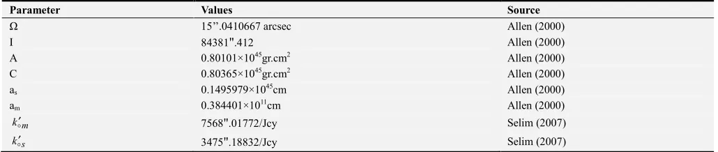
(87)6. Numerical Representation of Nutation Series
The numerical computations of the forced nutation for angular momentum axis eqns. (47), (48), (50), (51), (52), (53), (79), (80), (82), (83), (84), (85), (86) and (87) will be carried out by using the numerical coefficient in table 1 [10, 17].
Table 1. Numerical coefficients.
Parameter Values Source
Ω 15’’.0410667 arcsec Allen (2000)
I 84381".412 Allen (2000)
A 0.80101×1045gr.cm2 Allen (2000)
C 0.80365×1045gr.cm2 Allen (2000)
as 0.1495979×1045cm Allen (2000)
am 0.384401×1011cm Allen (2000)
m
k′ 7568".01772/Jcy Selim (2007)
s
k′ 3475".18832/Jcy Selim (2007)
Table 2. Coupling between affecting forces (Nutation in Longitude and Obliquity); Unit=0.001 mas.
Period (days) Nutation of Andoyer plane Longitude Nutation of equatorial plane Obliquity
andoyer oppolzer figlon andoyer Oppolzer figobli
-6798.36 0.00095 0.00029 0.00123 -0.00020 -0.00028 -0.00048
-3399.18 0.00000 0.00002 0.00003 0.00002 -0.00002 -0.00000
1305.47 -0.00000 0.00000 -0.00000 0.00000 -0.00000 -0.00000
409.23 0.00000 0.00000 0.00000 0.00000 -0.00000 0.00000
365.26 0.00000 -0.00000 0.00000 0.00000 0.00000 0.00000
212.32 -0.00000 0.00000 -0.00000 0.00000 -0.00000 -0.00000
182.62 -0.00003 -0.00014 -0.00016 -0.00014 0.00014 -0.00000
121.75 -0.00000 -0.00001 -0.00001 -0.00001 0.00001 -0.00000
117.54 -0.00000 0.00000 -0.00000 0.00000 -0.00000 -0.00000
-32.61 0.00000 -0.00000 0.00000 -0.00000 0.00000 -0.00000
29.53 -0.00000 0.00000 -0.00000 0.00000 -0.00000 -0.00000
-27.33 0.00000 0.00000 0.00000 0.00000 -0.00000 -0.00000
Table 3. Affecting forces separately (Nutation in Longitude and Obliquity); Unit=0.001 mas.
Period (days)
Free Rigid
Nutation of Andoyer plane longitude Nutation of equatorial plane Obliquity
andoyerlonr figlonr andoyeroblir figoblir
-6798.36 0.00000 0.00000 0.00000 0.00000
-3399.18 0.00000 0.00000 -0.00000 -0.00000
1305.47 -0.00000 -0.00000 -0.00000 -0.00000
409.23 0.00000 0.00000 -0.00000 -0.00000
365.26 0.00000 0.00000 0.00000 0.00000
212.32 -0.00000 -0.00000 -0.00000 -0.00000
182.62 -0.00000 -0.00000 0.00000 0.00000
121.75 -0.00000 -0.00000 0.00000 0.00000
117.54 -0.00000 -0.00000 0.00000 0.00000
-32.61 0.00000 0.00000 0.00000 0.00000
29.53 -0.00000 -0.00000 0.00000 0.00000
Table 3. Continued.
Period (days)
Tidal Forces
Nutation of Andoyer plane longitude Nutation of equatorial plane Obliquity
andoyerlont oplont figlont andoyeroblit opoblit figoblit
-6798.36 0.00096 0.00000 0.00096 0.00000 0.00028 0.00028
-3399.18 0.00000 0.00000 0.00000 0.00000 0.00002 0.00002
1305.47 -0.00000 0.00000 -0.00000 0.00000 0.00000 0.00000
409.23 0.00000 0.00000 0.00000 0.00000 0.00000 0.00000
365.26 0.00000 -0.00000 0.00000 0.00000 -0.00000 -0.00000
212.32 -0.00000 0.00000 -0.00000 0.000000 0.00000 0.00000
182.62 -0.00000 -0.00000 -0.00000 0.00043 -0.00027 0.00016
121.75 -0.00000 -0.00000 -0.00000 0.00002 -0.00001 0.00001
117.54 -0.00000 0.00000 -0.00000 0.00000 0.00000 0.00000
-32.61 0.00000 -0.00000 0.00000 0.00000 -0.00000 -0.00000
29.53 -0.00000 0.00000 -0.00000 0.00000 0.00000 0.00000
-27.33 0.00000 0.00000 0.00000 0.00000 0.00000 0.00000
7. Conclusion
Numerical of nutation series for the plane perpendicular to angular momentum vector and the plane perpendicular to figure axis of Earth will be carried out for the two cases of the present theories, tidal effect’s forces coupling with the geopotential and the other by neglect the coupling between affecting forces. As mention before, we taking the approximation triaxial symmetry of Earth and using the other numerical coefficient listed in table 1 (Numerical coefficients) [10, 17].
As we saw in Part 1 and 2
Tides are generated by the same forces, which cause nutation, but with the basic difference that the tidal effects depend on the elastic responses of the Earth, and in turn on the Earth’s internal structure.
In part 1, tidal disturbances cause vertical deformation not exceeding 0``. 009. The tidal distortion of the Earth’s figure appears as a displacement of the plane by a few centimeters. These changes are reflected as variations in the astronomical latitude (defined as the complement of the angle between the rotation axis and the local vertical). The geocentric latitude is also affected but to a lesser extent not exceeding 0.``003.
In part 2, we notes that tidal disturbance nearly neglected in case of free rotation of Earth, but the effected forces are that forces caused by gravitation of Moon and Sun which clear at the same periods as part 1 (periods -6798.36 and 182, 62) although the precession and nutation are less than in the case of coupling effects but they are clear.
Acknowledgements
Authors are grateful to the anonymous referee for helpful comments.
References
[1] Munck, W, H. and Macdonald, G. J. “The Rotation of the Earth’’. Cambridge (1960).
[2] Getino, J. and ferrandiz, J. M., A Hamiltonian theory for an
elastic earth: Canonical variables and kinetic energy, Celest. Mech. 49, 303 (1990).
[3] Getino, J. and ferrandiz, J. M., A Hamiltonian theory for an elastic earth: Elastic energy of deformation, Celest. Mech. 51, 17 (1991a). [4] Getino, J. and ferrandiz, J. M., A Hamiltonian theory for an
elastic earth: First order analytical integration, Celest. Mech. 51, 35 (1991b).
[5] Getino, J. and ferrandiz, J. M., A Hamiltonian theory for an elastic earth: Secular rotational acceleration, Celest. Mech. 52, 381 (1991c).
[6] Getino, J. and ferrandiz, J. M., On the effect of the mantle elasticity on the earth's rotation, Celest. Mech. 61, 117 (1995). [7] Sauchay, J. and Kinoshita, H., Comparison of new nutation
series with numerical integration, Celest. Mech. 52, 45 (1991). [8] Ferrandiz, J. M.; Navarro, J. F., Escapa, A.; and Getino, J., Earth’s Rotation: A Challenging Problem in Mathematics and Physics, Pure Appl. Geophys. 172, 57–74 (2015).
[9] Selim, H. H., Forced Nutation for The Rigid Earth Model At The First Order, NRIAG Journal of Astronomy and Geophysics, Special Issue, PP. 275-290 (2004).
[10] Selim, H. H., Hamiltonian of A Second Order Two- Layer Earth Model, Journal of The Korean Astronomical Society, 40, 49 (2007). [11] Capitaine, N.; Mathews, P. M.; Dehant, V.; Wallace, P. T.; Lambert, S. B., On the IAU 2000/2006 precession–nutation and comparison with other models and VLBI observations, Celest Mech Dyn Astronomy, 103 (2), 179 (2009).
[12] Malkin, Z., Joint analysis of celestial pole offset and free core nutation series , J. Geodesy, Volume 91, (7), 839 (2017). [13] Schindelegger M.; Einšpigel, D.; Salstein, D.; Böhm, J., The Global
S1 Tide in Earth’s Nutation, Surv Geophys, 37 (3), pp. 643 (2016). [14] Hori, G., Theory of General Perturbation with Unspecified
Canonical Variable, pub1. Astr. Soc. Japan, 18 (4), 287. (1966). [15] Kinoshita, H., Theory of the rotation of the rigid earth, Celest.
Mec, h. 15, 2. (1977).
[16] Getino, J., Forced nutations of a rigid mantle-liquid core Earth model, Geophysics J. Int., 122, 803-814, (2007).