Adv. Stat. Clim. Meteorol. Oceanogr., 2, 63–78, 2016 https://doi.org/10.5194/ascmo-2-63-2016
© Author(s) 2016. This work is distributed under the Creative Commons Attribution 3.0 License.
A comparison of two methods for detecting abrupt
changes in the variance of climatic time series
Sergei N. Rodionov
Climate Logic LLC, Superior, CO 80027, USA
Correspondence to:Sergei N. Rodionov ([email protected])
Received: 19 February 2016 – Revised: 7 May 2016 – Accepted: 2 June 2016 – Published: 24 June 2016
Abstract. Two methods for detecting abrupt shifts in the variance – Integrated Cumulative Sum of Squares
(ICSS) and Sequential Regime Shift Detector (SRSD) – have been compared on both synthetic and observed time series. In Monte Carlo experiments, SRSD outperformed ICSS in the overwhelming majority of the modeled scenarios with different sequences of variance regimes. The SRSD advantage was particularly apparent in the case of outliers in the series. On the other hand, SRSD has more parameters to adjust than ICSS, which requires more experience from the user in order to select those parameters properly. Therefore, ICSS can serve as a good starting point of a regime shift analysis. When tested on climatic time series, in most cases both methods detected the same change points in the longer series (252–787 monthly values). The only exception was the Arctic Ocean sea surface temperature (SST) series, when ICSS found one extra change point that appeared to be spurious. As for the shorter time series (66–136 yearly values), ICSS failed to detect any change points even when the variance doubled or tripled from one regime to another. For these time series, SRSD is recommended. Interestingly, all the climatic time series tested, from the Arctic to the tropics, had one thing in common: the last shift detected in each of these series was toward a high-variance regime. This is consistent with other findings of increased climate variability in recent decades.
1 Introduction
A concept of regime shifts, i.e., abrupt structural changes in climatic time series, has gained popularity in recent decades. Literature reviews (Beaulieu et al., 2012; Liu et al., 2016; Rodionov, 2005a) show that most of the effort in this area is directed towards changes in the mean, where numerous methods of shift (or change point) detection have been devel-oped. Changes in climate variability, and more specifically in variance, as a direct measure of variability, have received less attention, both in documenting those changes and devel-oping of methods for their detection. Thus, a comprehensive review of change point detection techniques for climate data by Reeves et al. (2007) has no mentioning of any methods for shifts in variance. It is known, however, that the potential impact of changes in climate variability may be as great or greater than the impact of changes in climate means (Hansen et al., 2012; Katz, 1988). There are indications that an in-crease in variance may signal impending shifts in ecosystems
(Carpenter and Brock, 2006) and regional climates (Wu et al., 2015).
Patterns of climate variability in the first half of the twen-tieth century were investigated by Schuurmans (1984), who showed that the minimum interannual variability of surface air temperature in western Europe occurred during the 1890– 1920 period. In central Europe, this minimum was less pro-nounced and shifted to a later period. For the Northern Hemi-sphere as a whole, the minimum frequency of temperature extremes occurred in the decade of 1920–1929.
were observed in Japan, East Coast (USA), Pacific North-west (USA), North-western Canada, northNorth-western Russia, and east-ern Australia. Huntingford et al. (2013) demonstrated that al-though fluctuations in annual temperature showed substantial geographical variation over the past few decades, the time-evolving standard deviation of globally averaged tempera-ture anomalies was stable. In contrast, Hansen et al. (2012) showed a widening of temperature probability density func-tions in the past 3 decades, especially in summer.
Summer extreme events, such as the heat waves of 2003 in western Europe (Chase et al., 2006) and of 2010 in east-ern Europe (Barriopedro et al., 2011), sparked debates about whether or not these were signs of global warming, the great-est impact of which could be due to changes in frequency of extreme events, and not just because of a simple increase in the mean. Although the probability of extreme events may be affected by changes in the mean state of the atmosphere (Rhines and Huybers, 2013), changes in the variance may be just as important. According to Katz and Brown (1992), the more extreme the event, the more important a change in the variability is relative to the mean. Indeed, Schär et al. (2004) calculated that the 2003 heat wave would be extremely un-likely given a change in the mean only. They showed that a recent increase in variability would be able to explain the heat wave.
Still, individual extreme events by themselves are not enough proof that the overall variance is on the rise. Those events may turn out to be just outliers that make the detection of regime shifts in the variance even more difficult. In fact, using very long and homogenized instrumental climatic time series Böhm (2012) found no change in variability during the past 250 years in Europe, not for pressure, not for tempera-ture, and not for precipitation. Interestingly, evidence from Greenland ice cores showed that an enhanced year-to-year temperature variability was probably more characteristic of past cold, rather than warm climates (Steffensen et al., 2008). Therefore, in spite of suggestions of higher variability in re-cent decades (Hansen et al., 2012), there is still considerable uncertainty as to whether it is actually occurring.
Conflicting reports and often statistically inconclusive re-sults underscore difficulties in detecting abrupt changes in the variance of climatic time series. As it will be shown in this paper, it is often hard to detect a regime shift even if the variance increases 2-fold from one period to another, partic-ularly for short time series, and even more so in the presence of outliers.
The most common statistical tool to study changes in cli-mate variability is the running standard deviation; however, this tool cannot be used in the case of abrupt transitions between variance regimes. Downton and Katz (1993) de-veloped a test to detect and adjust inhomogeneities in the variance of temperature time series. Their test uses a non-parametric bootstrap technique to compute confidence inter-vals for the discontinuity in variance. More recently, Killick et al. (2010) used a change point analysis to detect abrupt
changes in the variance of significant wave heights in the Gulf of Mexico. They adopted a penalized likelihood ap-proach using the Schwarz information criterion proposed by Yao (1988). Topál et al. (2016) examined the perfor-mance of three change point detection methods: (1) kink point (Matyasovszky, 2011), (2) modified cross-entropy (CE; Evans et al., 2011), and (3) change point model (CPM) framework (Hawkins and Zamba, 2005). The experiments were conducted with one white and one red noise series of sizen=200 with artificially modified last quarter of the se-ries to simulate a change point. When a detected change point was located within an “acceptance interval” (defined as±5 % ofnaround the true change point), it was considered as ac-curately found. The kink method tended to find not one, but two change points in variance within the acceptance interval, which was attributed to the fact that the method was origi-nally designed for abrupt changes in trend. The CE method was not able to recognize any changes in variance, regardless of the magnitude of a shift. The CPM method was the most accurate, but it turned out to be overly sensitive. When tested on 1000 normally distributed random white and red noise se-ries with no change point, the method found change points in more than 60 % of the series.
Currently, the most advanced methods of regime shift de-tection in the variance appear to exist in econometrics, espe-cially quantitative finance, where the concept of stock market volatility is very important. One of the most popular among those methods is the Iterated Cumulative Sum of Squares (ICSS) algorithm developed by Inclan and Tiao (1994). Whitcher et al. (2002) applied ICSS to test homogeneity of variance in time series of water levels in the Nile River. Using a version of the discrete wavelet transform, they confirmed that the point at which the test statistic in ICSS achieves its maximum value can be used to estimate the time of the un-known variance change.
The purpose of this paper is to compare ICSS with the Se-quential Regime Shift Detector (SRSD), a method developed by the author Rodionov (2005b). These two methods are de-scribed in Sect. 2. In Sect. 3, the methods are tested using Monte Carlo experiments with different sequences of vari-ance regimes, magnitudes of shifts and positions of change points. The effect of outliers is also evaluated. The real-world examples are presented in Sect. 4. The methods are ap-plied to climatic time series from different geographic zones, from the Arctic to the tropics. The results are summarized in Sect. 5.
2 Methods
2.1 Iterated cumulative sums of squares
Suppose{xi}, i=1, . . .nis a series of independent, normally
S. N. Rodionov: A comparison of two methods for detecting abrupt changes in climatic time series 65
Table 1. Percentages of total numbers of change points detected
by SRSD (p, 30, 2) in each series on average and hits of the true change pointc1=51. The regime variances areσj2=(1,2).
Change points detected
p 0 1 ≥2 Hits
0.05 57 41 2 4.5
0.1 41 54 5 5.9
0.3 13 65 22 7.7
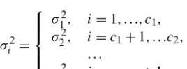
that experiences abrupt shifts at unknown time, i.e.,
σi2=
σ12, i=1, . . ., c1, σ22, i=c1+1, . . .c2,
. . .
σm2, i=cm−1+1, . . .n.
(1)
The task is to find the number of variance regimes mand locations of change pointscj, j=1, . . ., m−1. To solve this
task, Inclan and Tiao (1994) proposed to use the centered (and normalized) cumulative sum (CUSUM) of squares:
Dk=
CUSUMk
CUSUMn
−k
n, k=1, . . ., n, (2)
where CUSUMk=Pki=1xi2. The algorithm consists of
sev-eral steps, dividing time series{xi}into pieces and applying Dk to each of them iteratively.
Step 1. Calculate Dk(x[i1:i2]) for the entire time series,
i.e.,i1=1 andi2=n. Letk∗(x[i1:i2]) be the point at which maxk|Dk(x[i1:i2])|is obtained and let
M(i1:i2)=
p
(n−i1+1)/2|Dk(x[i1:i2])|. (3)
If M(i1:i2) is greater than the critical valueD∗ from Table 1 in Inclan and Tiao (1994), then there is a change point at k∗(x[i1:i2]) and proceed to step 2a. If M(i1:i2)< D∗, there is no evidence of variance changes in the series and the algorithm stops. For signif-icance levelp=0.05 (the level used in this paper) and 100 observations, the critical value D0∗.05=1.27. As the number of observation increases, the critical value also slightly increases. The asymptotic critical value is D0∗.05=1.358.
Step 2a. EvaluateDk(x[i1:i2]) for the first part of the se-ries from the beginning up to i2=k∗(x[i1:i2]). If M(i1:i2)> D∗, step 2a is repeated for a new (smaller) i2 until M(i1:i2)< D∗. When this occurs, the first point of change iskfirst=i2.
Step 2b. Now do a similar search for the second part of the series from the change point found in step 1 till the
end of the time series, i.e.,i1=k∗+1 and i2=n. If M(i1:i2)> D∗, step 2b is repeated using a new (larger) i1untilM(i1:i2)< D∗. When this occurs, the last point of change isklast=i1−1.
Step 2c. If kfirst=klast, there is just one change point. If kfirst< klast, keep both values as possible change points and repeat steps 1 and 2, but for the middle part of the series, i.e., i1=kfirst+1 and i1=klast. Each time steps 2a and 2b are repeated, the result can be one or two more change points. Callmthe number of variance regimes (m−1 change points) found so far.
Step 3. Check each possible change pointcj by calculating
Dk xcj−1+1:cj+1, j=1, . . ., m−1;c0=0,cm=
n. If M cj−1+1:cj+1> D∗, then keep the point; otherwise, eliminate it. Repeat step 3 until the number of change points does not change and the points found in each new pass are “close” (within two observations in our case) to those on the previous pass.
2.2 Sequential regime shift detector
The SRSD software package consists of three modules for detection of regime shifts in the mean, variance, and corre-lation coefficient (see www.climatelogic.com). The variance module, which is the focus here, was first described in Ro-dionov (2005b) and then, as part of a three-step procedure, in Rodionov (2015). Similar to ICSS, SRSD is a CUSUM-type method. An important difference is that ICSS is a retro-spective algorithm, whereas SRSD employs a sequential ap-proach. While ICSS can be applied only after all the data are collected, SRSD treats the data sequentially, one data point at a time. This allows for using SRSD for monitoring of regime shifts beyond the history period 1, . . ., n.
The SRSD algorithm is based on theF-test that compares the ratio of sample variance for the “current” regime,sj2to that for the “new” regime to be detected,sj2+1, with the criti-cal valueFcr:
F = s 2
j
sj2+1Fcr. (4)
HereFcris the value of theF-distribution withν1andν2 de-grees of freedom and a significance levelp(two-tailed test), Fcr=F(p/2, ν1, ν2). The degrees of freedom are calculated asν1=ν2=l−1, wherel is called the cutoff length, a pa-rameter that allows one to focus on certain timescales of vari-ance regimes. More about the effect ofpandlon regime shift detection in the next section.
For the new regime to be statistically significantly different from the current regime, variancesj2+1should be greater than
scr2↓, if the variance decreases, where
scr2 =
(
scr2↑=sj2Fcr,
scr2↓=sj2/Fcr.
(5)
When a new observation xi arrives at timei, it is checked
againstscr2. Ifxi2falls outside the interval[scr2↓s2
↑
cr ], this point in time is marked as a potential change pointc∗, and the sub-sequentl−1 data points are used to test the null hypothesis of no regime shift. The decision rule is based on the residual sum of squares index (RSSI):
RSSI=1 l
k
X
i=c∗
(xi2−scr2), k=c∗, c∗+1, . . ., c∗+l−1. (6)
If during this testing period RSSI remains positive in the case of increasing variance, or negative in the case of decreasing variance, the null hypothesis of a constant variance is re-jected, and c∗ becomes a true change pointcj+1. If RSSI changes its sign, the test for c∗ stops, because the null hy-pothesis cannot be rejected. The observation xi is included
in the current regimej, and the regime variancesj2is recal-culated incrementally as in Finch (2009):
snew2 =njs 2 old+x
2
i
nj+1
, (7)
wherenj is the length of regimej before adding a new
ob-servation.
Handling outliers
An outlier is a data point, whose value is substantially differ-ent from the other data points in a sample. The presence of outliers can lead to large errors in estimates of regime statis-tics and greatly affect the timing of regime shifts. This is par-ticularly true for the variance, because the data values are squared.
When dealing with outliers, it is desirable to leave an ob-servation intact if it falls within a “normal” range of varia-tion, and assign it a small weight if it is outside that range (Huber, 1981). In SRSD, each observationxi in the current
regime j is assigned a Huber-type weightwi, which is
de-fined as
wi =min
1, hscale |xi|
, (8)
wherehis a tuning constant and “scale” is first estimated as the median absolute deviation (MAD):
MAD=median (|xi|), i=cj, cj+1, . . ., c∗−1. (9)
After the weights are estimated, the regime variance is cal-culated as
sj2=
Pc∗−1
i=cjw 2
ix
2
i
V1−(V2/V1)
, (10)
where
V1=
c∗−1
X
i=cj
wi2, V2=
c∗−1
X
i=cj
w4i. (11)
To improve accuracy of the estimates, the weights are recal-culated, this time using the weighted standard deviation as scale. Then the regime variance is recalculated one more time as in Eq. (10) using more accurate weights.
When a potential regime shift is tested by calculating RSSI, the weights for data pointsi=c∗, c∗+1, . . ., c∗+l−1, are assigned as
wi=min
1, hsj±scr |xi|
. (12)
If the test cannot reject the null hypothesis andxi is added to
the current regime, the weight for this observation is recalcu-lated using Eq. (8) with scale=sj. The weighted version of
Eq. (7) for incremental recalculation of the regime variance is
snew2 =V1s 2
old+wi2x2i
V1+wi2
. (13)
3 Monte Carlo experiments
Both the ICSS and SRSD algorithms were implemented by the author as VBA (visual basic for applications) macros for Microsoft Excel. The majority of experiments were per-formed using samples of size n=100, which is a typical length (in years) of instrumental climatic time series. For each test, 10 000 samples of random normally distributed numbers are generated with zero mean and one or two change points in the variance. A change points is defined as in SRSD, i.e., as the first point of a regime. Since ICSS defines a change point as the last point of a regime, all the change points de-tected by ICSS are shifted one step forward. A total of four groups of experiments were conducted: (1) with one change point located in the middle and closer to the ends of time se-ries, (2) with two change points and different combinations of variance regimes, (3) with outliers, and (4) with autocor-relation. Before starting comparing the two methods, it is important to clarify the role of the significance levelp and cutoff lengthlon regime shift detection by SRSD.
3.1 The effect of tuning parameterspandl
As shown above, the performance of SRSD can be controlled by three parameters: the significance levelp, cutoff lengthl, and Huber’s tuning constanth. This will be denoted as SRSD (p,l,h). Let us clarify the role of the first two parameters. The Huber’s tuning constant becomes really important only in the presence of outliers.
S. N. Rodionov: A comparison of two methods for detecting abrupt changes in climatic time series 67
0 1 2 3 4 5 6 7 8 9
1 6 11 16 21 26 31 36 41 46 51 56 61 66 71 76 81 86 91 96
Fr
eq
u
en
cy
(
%
)
Data point
0.05 0.1 0.3
Figure 1. Frequency distribution of change points detected by
SRSD (p, 30, 2) for three different values of p: 0.05, 0.1, and 0.3. The true change point is c1=51 and regime variances are
σj2=(1,2).
ofp, SRSD becomes sensitive to smaller and smaller shifts in the variance, thus reducing the probability of a type II error (false negative). On the other hand, the probability of a type I error (false positive) increases, leading to spurious shifts. This is demonstrated in Fig. 1 that shows the frequency of shift detection for different values of p. The true change point is located ati=51 and the variance doubles from the first regime to the second. At p=0.05, the percentage of hits (change points detected exactly ati=51) is 4.5. In 57 % of the time, SRSD fails to detect any shift in the series (Ta-ble 1). Aspincreases, the percentage of hits also increases, but the tails of the distribution in Fig. 1 become heavier. It is important to note, that since SRSD is a sequential algo-rithm, the frequency of change points found at the end of the series increases substantially, as illustrated forp=0.3. But these are only potentialchange points that may or may not pass the test. Therefore, when comparing SRSD and ICSS, only the fully resolved change points were considered. More specifically, the numbers of change points detected in each series (as presented in Tables 1–5) were counted for the pe-riod 1, . . ., n−lfor both methods.
The choice ofpdepends on the magnitude of shifts. Fig-ure 2 shows that as the magnitude of a shift increases, the accuracy of shift detection is increasing faster for smallerp. Thus, if the ratio of variances between two adjacent regimes is greater than 4, it is better to usep=0.05, which provides better accuracy of detection and fewer false positives, than p=0.1 orp=0.3. If the goal is to detect shifts of smaller magnitude, the choice ofp=0.1 or higher would be appro-priate. The target probability level p can be considered as the upper limit of the desired significance level of the shifts; thepvalues, calculated after all shifts in a series have been detected, are usually lower.
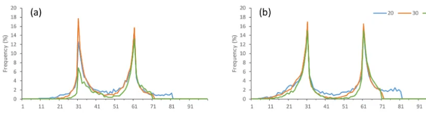
The cutoff lengthl controls the timescale of the detected regimes. As an example, Fig. 3a shows the results for time
0 5 10 15 20 25 30 35 40
2 3 4 5 6 7 8
Fr
eq
u
en
cy
(
%
)
Variance ratio
0.05 0.1 0.3
Figure 2.Percentage of hits as a function of the variance ratio be-tween two regimes (σ22/σ12) for different values ofpin SRSD (p, 30, 2).
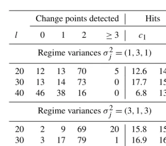
Table 2.Percentages of total numbers of change points detected by
SRSD (0.1,l, 2) in each series on average and hits of the true change pointscj=(31,61).
Change points detected Hits
l 0 1 2 ≥3 c1 c2
Regime variancesσj2=(1,3,1)
20 12 13 70 5 12.6 14.5
30 13 14 73 0 17.7 15.7
40 46 38 16 0 6.8 13.3
Regime variancesσj2=(3,1,3)
20 2 9 69 20 15.8 15.8
30 3 17 79 1 16.9 16.5
40 21 69 10 0 15.0 15.0
series with three variance regimes,σj2=(1,3,1), and two change points,cj =(31,61). The best results were obtained
Figure 3.Frequency distributions of change points detected by SRSD (0.1,l, 2) with three different values ofl: 20, 30, and 40. The true change points arecj=(31,61), and regime variances are(a)σj2=(1,3,1) and(b)σj2=(3,1,3).
Table 3.Percentages of total numbers of change points detected by SRSD (p,l, 2) and ICSS in each series on average in the case of one true change point. The corresponding frequency distributions of the detected change points are presented in Fig. 4.
SRSD ICSS
Fig. 4 c1 σj2 p l 0 1 ≥2 0 1 ≥2
a 51 (1, 2) 0.2 40 35 64 1 42 55 3
b 51 (2, 1) 0.2 40 20 79 1 41 57 2
c 25 (1, 3) 0.05 20 28 59 13 53 46 2
d 90 (1, 3) 0.1 20 67 19 14 51 47 2
e 21 (3, 1) 0.1 20 8 69 23 22 76 2
f 71 (3, 1) 0.1 25 15 71 14 28 69 3
both methods. The values ofl are used a bit smaller than a specified regime length, because in practice the exact length of regimes in a series is usually unknown. In some cases, the results for two or three different values ofl are shown to demonstrate the effect of this parameter. When working with real time series it is recommended to experiment with different values ofp andl, in the same way as it is always advised in spectral analysis to try different window shapes and sizes when smoothing a periodogram.
Before discussing the results of testing with any change points, it is important to show that the methods are not overly sensitive in finding change points when no such points are present in a series. For this purpose, 10 000 white noise time series of size n=100 were generated. With p set to 0.05, ICSS finds zero change points in 96 % of the series. The re-sults for SRSD with the samepvary depending onl, increas-ing from 83 % forl=20 to 98 % forl=50.
3.2 Series with one change point
The first two experiments were performed with a change point positioned in the middle of the series (c1=51), while the variance either increased from one to two (Fig. 4a) or decreased from two to one (Fig. 4b). In both cases, SRSD outperformed ICSS in terms of the correct number of change points detected and percentage of hits (Table 3). Note that ICSS found no shifts at all in about 40 % of the generated series. Some variations inldid not affect much the principal
results. For example, whenlwas reduced from 40 to 30, with all other parameters being equal, the percentages of hits and numbers of time series with one shift detected by SRSD, re-mained practically the same in both cases of increasing and decreasing variance. What changed was the percentages in two other categories in Table 3, that is, with zero and two or more points detected; the former decreased by about 7–10 %, while the latter increased by the same amount.
It is important that the modes of frequency distributions in Fig. 4a and b coincide exactly with the positions of true change points; however, the percentages of hits are only about 8 % for SRSD and 6 % for ICSS. These small num-bers underscore the difficulty of detecting a regime shift even when the variance doubles. This sentiment is echoed by Kil-lick et al. (2010), who tested the penalized likelihood method in a similar Monte Carlo experiment with sample sizes of 200 points. They concluded that satisfactory power of their method was obtained only for variance ratios greater than three.
S. N. Rodionov: A comparison of two methods for detecting abrupt changes in climatic time series 69
Figure 4.Results of Monte Carlo experiments with one change point. The parameters of SRSD used in each of the experiments are given in
Table 3.
relatively high, which delays a shift detection. In the case of SRSD, the frequency distribution is more symmetric, be-cause the probability of a potential change point passing the test increases toward the true change pointc1.
When the variance increases from one regime to another, ICSS performs particularly poor if the change point is located closer to the beginning of a time series. In an experiment with a change point atc1=25, and a regime shift from one to three, ICSS found one change point 46 % of the time, but these change points were all over the place, with only 1.1 % of hits of the true change pointc1(Fig. 4c). In contrast, ICSS performed better, being on par with SRSD, when a change point was shifted toward the end of a time series, unless it was too close to the end. Since SRSD is a sequential method, designed to work in a monitoring mode, it is not surprising that it outperformed ICSS when a change point was placed at c1=90 (Fig. 4d).
When the variance decreases from one regime to another, ICSS performs much better if a change point is shifted
to-ward the beginning of a time series than toto-ward the end. In an experiment when a change point was placed atc1=21, ICSS and SRSD showed similar results (Fig. 4e), but when a change point was moved toc1=71, the percentage of hits for SRSD was more than twice that of ICSS (Fig. 4f).
3.3 Series with two change points
In this group of experiments, the locations of change points remain constant atcj=(34,67). The main goal here is to test
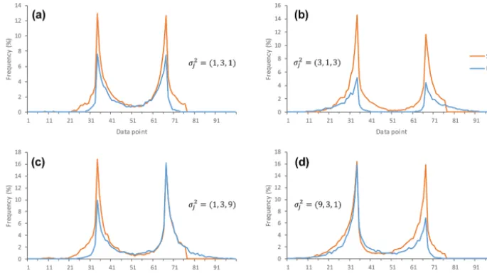
Figure 5.Results of Monte Carlo experiments with two change pointscj=(34,67). The parameters of SRSD used in each of the experiments
are given in Table 4.
Table 4.Percentages of total numbers of change points detected by SRSD (p, 25,h) and ICSS in each series on average in the case of two
true change pointscj=(34,67). The corresponding frequency distributions of the detected change points are presented in Fig. 5.
SRSD ICSS
Fig. 5 σj2 p h 0 1 2 ≥3 0 1 2 ≥3
a (1, 3, 1) 0.05 2 23 15 62 0 55 5 39 1
b (3, 1, 3) 0.05 2 17 27 56 0 62 16 21 1
c (1, 3, 9) 0.2 3 0 28 69 3 0 54 44 2
d (9, 3, 1) 0.2 3 0 9 84 7 0 64 34 2
The situation becomes even worse for ICSS, if the lower variance regime is in the middle; i.e.,σj2=(3,1,3) (Fig. 5b). In this case, ICSS correctly detected two change points in only 21 % of the series, and the accuracy of detection is about one-third of that for SRSD. This is consistent with the results of Inclan and Tiao (1994), who found that ICSS performs best when the larger variance is in the middle, and its perfor-mance deteriorates in the opposite situation.
The most difficult situation, according to Inclan and Tiao (1994), is when the variances change in a monotone way, i.e., the variance increases at the first change point and increases again at the second change point. They estimate that, if this is the case, then it is necessary to have 500 or more observations for ICSS to be able to detect two change points in more than half of the time. Indeed, for a sequence of variancesσj2=(1,3,9) (Fig. 5c), ICSS detected two change points in only 44 % of the series vs. 69 % for SRSD (Table 4). Especially problematic for ICSS was the detection of the first change point,c1, which was correctly detected in only 9.9 % of the series, compared to 16.8 % for SRSD. The detection statistics forc2is about the same for both methods.
When the variance decreased in a monotone way asσj2= (9,3,1), ICSS detected the first change point more often than the second one, while SRSD detected both change points with about the same accuracy (Fig. 5d). The difference in the frequency of detection of two change points simultane-ously between the two methods is quite substantial: 84 % for SRSD and only 34 % for ICSS (Table 5).
3.4 Series with outliers
S. N. Rodionov: A comparison of two methods for detecting abrupt changes in climatic time series 71
0 5 10 15 20 25 30 35
1 11 21 31 41 51 61 71 81 91
Fr
eque
nc
y (
%
)
Data point
𝑐𝑗= (34,68)
𝜎𝑗2= (6,1,6)
𝑥50∗ = 6
0 5 10 15 20 25 30 35
1 11 21 31 41 51 61 71 81 91
Fr
eque
nc
y (
%
)
Data point
𝑐𝑗= (34,68)
𝜎𝑗2= (6,1,6)
No outliers 0
5 10 15 20 25 30 35
1 11 21 31 41 51 61 71 81 91
Fr
eque
nc
y (
%
)
Data point
𝑐1= 34
𝜎𝑗2= (6,1)
𝑥65∗ = 6
0 10 20 30 40 50 60 70 80
1 11 21 31 41 51 61 71 81 91
Fr
eque
nc
y (
%
)
Data point
SRSD ICSS 𝑐1= 34
𝜎𝑗2= (6,1)
𝑥45∗ = 6
(a) (b)
(c) (d)
Figure 6.Results of Monte Carlo experiments with an outlierxi∗=6. The parameters of SRSD used in each of the experiments are given in
Table 5.
Table 5.Percentages of total numbers of change points detected by SRSD (0.05,l, 2) and ICSS in each series on average in the case of
experiments with an outlierxi∗=6. The corresponding frequency distributions of the detected change points are presented in Fig. 6.
SRSD ICSS
Fig. 6 cj σj2 Outlier l 0 1 2 ≥3 0 1 2 ≥3
a 34 (6, 1) 65 25 0 88 12 0 1 54 4 41
b 34 (6, 1) 45 25 0 83 17 0 0 94 3 3
c (34, 68) (6, 1, 6) N/A 20 0 4 90 6 31 4 61 4
d (34, 68) (6, 1, 6) 50 20 2 10 85 3 63 21 14 2
The effect of an outlier was even more dramatic when it was placed closer to the true change point (Fig. 6b). In this case, ICSS detected one change point in 94 % of the series, but the overwhelming majority of those change points were found ati=45 (position of the outlier), not ati=34 (true change point). Again, the results for SRSD were not affected, except for a small bump in the frequency distribution ati= 45 (Fig. 6b).
In some situations, an outlier may not cause a spuri-ous shift, but rather a drastic deterioration of ICSS perfor-mance. For example, Fig. 6c and d show the results for the same variance regimes, σj2=(6,1,6), and change points, cj=(34,68). The only difference is that, in the latter case,
there was an outlier at i=50. As a result, both the sensi-tivity and accuracy of ICSS was drastically reduced. In the majority of the series (63 %), ICSS found no change points at all, and the percentage of hits forc1andc2was reduced to 5.2 and 4.4, respectively. The performance of SRSD was not seriously affected by the outlier.
3.5 Series with autocorrelation
The majority of the methods for change point detection assume that the data are independent and identically dis-tributed. This is not always true for climatic time series that may contain autocorrelation that often exhibits itself in the form of red noise (Rudnick and Davis, 2003). Lund et al. (2007) investigated the effect of serial autocorrelation on change point detection in the case of shifts in mean. They found drastic performance degradation even in the presence of minor positive lag-1 autocorrelation coefficient (ρ). Thus, atρ=0.15, the rate of type I errors (too many false change points) was three times as large as that atρ=0.
Figure 7. Percentage of hits as a function of the autocorrelation coefficient in experiments with one change point atc1=51 between
two variance regimesσj2=(1,3). The parameters for SRSD were set asp=0.1,l=40, andh=2.
To examine the effect of autocorrelation on detection of regime shifts in variance, 10 000 first-order autoregressive series of lengthn=100 were generated. A change point was positioned in the middle of the series (c1=51), while the variance increased from 1 to 3. Under this settings, the hit rates for white noise series (ρ=0) were about the same for both SRSD (0.1, 40, 2) and ICSS (Fig. 7). With an increase of ρ, the hit rates start decreasing, but first quite slowly. At ρ=0.3, the decrease is only 8 % for SRSD and 11 % for ICSS. Asρincreases further, the decrease in hit rates accel-erates; atρ=0.7, it drops by 45 % for SRSD and by 57 % for ICSS. Also, forρ≥0.6, the mode of frequency distribution of change points detected by ICSS does not coincide with the position of the true change point atc1=51, being shifted 1– 2 points forward. It should be noted that while the sensitivity or detection power of the methods deteriorates with the in-crease ofρ, the rate of spurious change points, expressed by the tails of the frequency distribution around the true change point (not shown), remains about the same. Apparently, the effect of serial autocorrelation on detection of regime shifts in variance is less dramatic than in mean.
4 Examples of climatic time series
4.1 Arctic Ocean sea surface temperature
In recent decades, the Arctic has been warming faster than other parts of the globe, a phenomenon known as Arctic amplification. Some observational analyses found evidence for a “wavier” jet stream in response to rapid Arctic warm-ing (Francis and Vavrus, 2015), which, in turn, may lead to greater temperature variability in the Arctic. Figure 8a shows monthly sea surface temperature (SST) anomalies for the Arctic Ocean (65–90◦N), based on the NOAA optimum interpolation SST data set. This data set (a.k.a. Reynolds OI.v2) is compiled using observations from ship inlets, buoys (both moored and drifting), and from satellites covering the
Figure 8. Arctic Ocean SST, November 1981–December 2015:
(a)SST anomalies (deviations from the period mean values for each month) and the LOWESS curve with a smoothing parameter of 0.1; (b)residuals (after removing the LOWESS curve and prewhitening) with two change points, December 1996 and July 2007, detected by SRSD (0.05, 120, 3). ICSS detected the same change points plus a third change point in September 2009 with a shift toward lower variance.
period from late 1981 to the present. It is available from the National Centers for Environmental Information (NCEI) web site at https://www.ncdc.noaa.gov/oisst.
Apart from an obvious warming trend in Fig. 8a, one can notice that SST fluctuations in recent years have become more intense. The exact cause of increased SST variabil-ity are beyond the scope of this paper, but this time series is a good example to test the regime shift detection algo-rithms. First, it is necessary to detrend the SST series that can be done in a number of ways, depending on the re-searcher’s view on what constitutes a trend. For this example, the LOWESS (local-weighted regression) technique (Cleve-land and Devlin, 1988) was used with a smoothing parame-ter of 0.1. When the LOWESS curve was subtracted from the SST anomalies, the residuals still contained a strong autocor-relation (red noise); therefore, a prewhitening was needed. Given the ordinary least squares estimate ofρ=0.72, the prewhitening was performed asei=xi−0.72xi−1.
The result of the application of SRSD (0.05, 120, 3) to time series{ei}is presented in Fig. 8b. Three variance regimes
sig-S. N. Rodionov: A comparison of two methods for detecting abrupt changes in climatic time series 73
nificant, especially the second one, with the observedp val-ues of 1.2×10⁻⁴and 5.5×10⁻⁹, respectively.
The ICSS algorithm found three change points, two of which coincided with those found by SRSD, and the third one was in September 2009. Formally, based on theF test, the difference in the variances for two regimes, July 2007– August 2009 (0.021) and September 2009–November 2015 (0.007), is statistically significant at p=3.2×10⁻⁴. The change point in September 2009 was not selected by SRSD for two reasons. First, the period July 2007–August 2009 is only 27 months, i.e., much shorter than the used cutoff length of 120 months. Second, given the Huber’s tuning constant of 2, the weighted variance for this short regime is only 0.012, which makes the difference between the two regimes, statis-tically insignificant.
4.2 Arctic oscillation
The Arctic oscillation (AO) is defined as the first empiri-cal orthogonal function (EOF) of sea level pressure (SLP) in the Northern Hemisphere (20–90◦N; Thompson and Wal-lace, 1998). Instead of SLP, the EOF analysis is often per-formed using monthly mean 1000 hPa height anomaly data to obtain the AO loading pattern (first EOF). The AO index is then calculated by projecting the AO loading pattern to the daily anomaly 1000 hPa height field over 20–90◦N. The monthly index values from January 1950 to the present are available from the NCEI website at https://www.ncdc.noaa. gov/teleconnections/ao/.
Broadly speaking, positive values of the AO index indi-cate zonal atmospheric flow, while negative values suggest increased meridional circulation with ties to cold air advec-tion into the midlatitudes (Thompson and Wallace, 2000). Analyzing variability of the winter (DJF) AO index, Feld-stein (2002) calculated that the ratio of its variance for the 1967–1997 time period to that for the 1899–1967 period was 2.02 and concluded that it was well in excess of what was to be expected if all of the interannual variability was due to atmospheric intraseasonal stochastic processes. Other stud-ies (Hanna et al., 2015; Woollings et al., 2010) argue that AO variability is most likely a result of atmospheric internal vari-ability, although it can be an early sign of destabilization of the polar jet stream and an increased susceptibility to exter-nal sources (Overland and Wang, 2015). Firm attribution of recent increased circulation variance is currently not possible (Trenberth et al., 2015).
Using the data since 1950, Overland and Wang (2015) no-ticed that the past decade showed the most variability in AO extremes for the month of December. Since they used the 9-year-running standard deviations, the timing of the transition to a high-variance regime was rather vague. Figure 9a shows the result of the application of SRSD (0.1, 25, 2) to the time series of December AO index, 1950–2015. Note that the lag-1 autocorrelation coefficient for this series is close to zero; therefore, no prewhitening is needed. The same is true for all
-3.0 -2.0
-1.0 0.0 1.0 2.0
3.0
1950 1960 1970 1980 1990 2000 2010
In
d
ex
v
a
lu
es
Arctic oscillation
-4.0 -3.0 -2.0 -1.0 0.0 1.0 2.0 3.0 4.0
Jan-95 Jan-97 Jan-99 Jan-01 Jan-03 Jan-05 Jan-07 Jan-09 Jan-11 Jan-13 Jan-15
In
d
ex
v
a
lu
es
Time of observation
(b) Monthly (a) December
Figure 9.The Arctic oscillation index:(a)December values, 1950–
2015, with a change point in 2005 detected by SRSD (0.1, 25, 2); (b)monthly values, January 1995–December 2015, with a change point in April 2009 detected by SRSD (0.05, 120, 2) and ICSS.
other climatic time series analyzed below. The AO index con-tains one change point in 2005 that separates two regimes: (1) 1950–2004, with the variance of 0.91, and (2) 2005–2015, with the variance of 2.71. The latter includes the record and near-record high values in 2006 and 2011, respectively, as well as the record and near-record low values in 2009 and 2010, respectively. The difference in the variance for these two regimes is statistically significant atp=0.009, based on the two-tailedF test.
As noted in Sect. 3, if a change point is shifted toward the end of time series, ICSS performs better when the variance increases, then when it decreases. Nevertheless, ICSS failed to detect any change points in the December AO index, prob-ably because the time series was too short for that method and the change point was too close to the end.
Both methods, however, were able to detect exactly the same change point in the monthly series of the AO in-dex, January 1950–December 2015 (Fig. 9b). The change point in April 2009 marks the transition from a low-variance regime (s12=0.83) to a high-variance regime (s22=1.69). Thepvalue for this regime shift is 1.1×10⁻⁴.
4.3 Temperature in the midlatitudes
-1.5 -1.0 -0.5 0.0 0.5 1.0 1.5 2.0 -3.0 -2.0 -1.0 0.0 1.0 2.0 3.0 4.0
1897 1907 1917 1927 1937 1947 1957 1967 1977 1987 1997 2007
SD
SA
T
Winter (DJF) SAT in Minneapolis
SAT first differences SD
Figure 10.First differences of winter (DJF) SAT anomalies in
Min-neapolis, MN, along with the 13-year-running standard deviations and two change points (1946 and 1980) detected by SRSD (0.1, 35, 3).
this pattern of temperature variability was characteristic of not just eastern Minnesota. The period of low temperature variability in the late 1960s–early 1970s occurred more or less simultaneously over the contiguous United States. Us-ing more recent gridded temperature data, HuntUs-ingford et al. (2013) examined changes to standard deviations before and after 1980. Although this change point year was se-lected without explicit testing, their map showed prominent changes over the midlatitudes for both hemispheres, with large parts of Europe and North America experiencing in-creased variability in more recent decades.
To illustrate the temporal pattern of changes in tempera-ture variability noticed by Skaggs et al. (1995), a homog-enized monthly temperature data set for Minneapolis, MN, was obtained from the Goddard Institute for Space Stud-ies (GISS) at http://data.giss.nasa.gov/gistemp/station_data/. Figure 10 shows the first differences of mean winter (DJF) temperature for that station for the period 1897–2015, along with the 13-year-running standard deviations. Using the first differences is a simple way of eliminating a trend in the mean and focus on variability. The running standard deviations ex-hibit a general decline toward the middle of the series and an increase in more recent decades. Although running devi-ations are useful in depicting trends in variability, they make it hard to pinpoint the exact locations of regime shifts. Ap-plying SRSD (0.1, 35, 3) to this time series revealed three temperature regimes with two change points, 1946 and 1980. During the first regime shift the variance decreased about 50 %, from 1.59 to 0.74. The second regime shift was more prominent; the variance jumped 3-fold to 2.32. The p val-ues for the shifts were 0.02 and 0.001, respectively. Despite the high statistical significance of these shifts, ICSS failed to detect any of them.
A significant increase in summer temperature variability was also observed at numerous European stations (Della-Marta et al., 2007; Parey et al., 2009; Yiou et al., 2009). For example, Della-Marta et al. (2007) found that over the period from 1880 to 2005 the length of summer heat waves over
-5.0 -4.0 -3.0 -2.0 -1.0 0.0 1.0 2.0 3.0 4.0 5.0
Jan-50 Jan-60 Jan-70 Jan-80 Jan-90 Jan-00 Jan-10
N o rm a li ze d a n o m a li es
Monthly SAT in western Europe
-5.0 -4.0 -3.0 -2.0 -1.0 0.0 1.0 2.0 3.0 4.0 5.0
Jan-50 Jan-60 Jan-70 Jan-80 Jan-90 Jan-00 Jan-10
N o rm a li ze d a n o m a li es
Time of observation
(a) Shifts in mean
(b) Shifts in variance
Figure 11.(a)Normalized (by standard deviations) monthly
sur-face air temperature (SAT) anomalies in western Europe (45–50◦N, 0–10◦E) and regime shifts in the mean detected by SRSD (0.05, 120, 2). The change points are February 1962 and August 1987; (b)Residuals after removing the stepwise trend in the mean and regime shifts in the variance detected by SRSD (0.1, 120, 2) and ICSS. The change points are July 1971 and September 2001.
western Europe doubled and the frequency of hot days al-most tripled. This trend of increasing temperature variability is projected to continue and even intensify in the 21st century (Fischer et al., 2012).
S. N. Rodionov: A comparison of two methods for detecting abrupt changes in climatic time series 75
the change points between them in July 1971 and September 1981 (Fig. 11b). The pvalues for the shifts in variance are 0.007 and 7.6×10⁻⁵, respectively.
4.4 El Niño–Southern Oscillation
The magnitude of El Niño–Southern Oscillation (ENSO) events has varied significantly over time, with multidecadal periods of strong and weak variability. Trenberth and Hoar (1996) noted strong ENSO variations from 1880 to the 1920s, and after about 1950 and, except for a strong event during 1939–1942, weaker variations from the mid-1920s to 1950. Exceptional ENSO variability can also be found in long ENSO-proxy records (Dunbar et al., 1994). Those periods usually coincided with large pre-industrial cli-mate variations (Quinn and Neal, 1992). More recently, Hu et al. (2013) investigated an interdecadal shift in the variability and mean state of the tropical Pacific Ocean within the con-text of changes in ENSO. They concluded that, compared with 1979–1999, the interannual variability in the tropical Pacific was significantly weaker in 2000–2011.
The ability of SRSD and ICSS to detect periods of high and low variability of ENSO was tested on the cold tongue index (CTI), one of the longest ENSO indices. The index is defined as the average SST anomaly over the region 6◦N–
6◦S, 180–90◦W minus the global mean SST. The index val-ues are available from the University of Washington, Seattle, WA (http://research.jisao.washington.edu/enso/). According to the website, the global mean SST anomaly is subtracted from the CTI in order to remove a step shift upward at the onset of World War II when the composition of the marine observations largely changed from bucket to engine intake measurements and to lessen the secular trend in the time se-ries that has been associated with global warming. Appar-ently, this has led to overcorrection of the CTI, because now there is a statistically significant (p=0.03) step shift down-ward in 1943, as detected by SRSD (Fig. 12a).
Figure 12b shows the residuals (deviations from the regime means) and two change points detected by SRSD (0.05, 35, 3). These change points separate three variance regimes: (1) high-variance regime (s12=0.82) in 1876– 1919, (2) low-variance regime (s22=0.42) in 1920–1982, and (3) high-variance regime (s32=1.05) that started with a powerful El Niño event of 1982–1983. Thep values are p=0.01 for the differences in variances between regimes one and two, andp=0.002 between regimes two and three. Despite the statistical significance of the shifts, ICSS failed to detect any of them.
5 Summary and conclusions
Changes in the variance of climatic time series are starting to attract more attention, especially from the perspective of global warming, because changes in the variance may have greater impact on temperature extremes than changes in the
-2.0 -1.5 -1.0 -0.5 0.0 0.5 1.0 1.5 2.0 2.5 3.0
1876 1891 1906 1921 1936 1951 1966 1981 1996 2011
Cold tongue index
-2.0 -1.5 -1.0 -0.5 0.0 0.5 1.0 1.5 2.0 2.5 3.0
1876 1891 1906 1921 1936 1951 1966 1981 1996 2011
Time of observation
(b) Shifts in variance (a) Shift in mean
Figure 12.(a)Mean winter (DJF) cold tongue index, 1876–2011,
showing a step shift downward in 1943 as detected by SRSD (0.1, 35, 3);(b)Residuals after removing the stepwise trend in the mean and regime shifts in the variance detected by SRSD (0.05, 35, 3) with change points in 1920 and 1983.
mean. In these circumstances, statistical methods capable of detecting shifts in the variance regimes are needed. A review of climate literature reveals that there are just a few practical methods available for that purpose and their applications are very limited so far. The situation is much more advanced in the area of econometrics, but the methods developed there need to be tested on climatic time series, which have their own specifics, such as a relatively short length and smaller magnitudes of shifts.
a sense of timescales of the regimes and magnitudes of shifts between them. Using this information will help to tune up SRSD for further analysis.
An important difference between the methods is that SRSD has an internal mechanism for dealing with outliers. Due to the lack of such mechanism in ICSS, Inclan and Tiao (1994) suggested complementing their procedure with some other procedure for outlier detection. It is better, how-ever, to combine these procedures, rather than do them sep-arately, one at a time, because an outlier in a low-variance regime may not be considered as such in a high-variance regime.
A comparison of the two methods was first implemented using Monte Carlo simulations with series of 100 points, which is a typical length (in years) of instrumental climatic time series. An interesting feature of ICSS is that it performs poor if a change point is located in the first half of a time se-ries when the variance increases from the first regime to the second, or if a change point is in the second half of the series when the variance decreases. In contrast, ICSS performs bet-ter in the opposite types of situations, that is, when a change point is in the first half of a series in the case of decreasing variance, or it is in the second half in the case of increasing variance. With two change points, ICSS detects the second point much more often than the first one if the variance in-creases in a monotone way, that is, from the first regime to the second and then again to the third. If the variance de-creases in a monotone way, ICSS more often selects the first change point than the second one. As for SRSD, it detects both change points with about the same degree of accuracy, regardless of the way the variance changes. Overall, SRSD outperforms ICSS in the overwhelming majority of the mod-eled situations. The only case when the two methods showed similar results was when a change point was located off the center of the series toward the end, but not too close to the end. For time series longer than 100 points, ICSS performs better, but it takes 500 or more points before it starts showing the results on par with SRSD. The experiments with series of more than 100 points, however, were very limited.
Some applications of ICSS for econometric time series have shown that it tends to overstate the number of actual change points in the variance (Fernández, 2004). This is probably only true for relatively long time series. As shown here, for time series of 100 points, ICSS rather tends to un-derstate the actual number of change points, and in many cases fails to find any change points at all.
When time series contain outliers, SRSD has a clear ad-vantage over ICSS. The effect of outliers on ICSS is quite interesting and may vary depending on both the absolute po-sitions of outliers in the series and their popo-sitions in relation to the true change points. Most commonly, ICSS finds spu-rious change points at the positions of outliers, but just the presence of outliers can also make ICSS grossly overstate the total number of change points in the series. The closer an outlier to a true change point, the more often it is
mis-takenly selected instead of a true change point. If an outlier is positioned between two change points, it may not cause a spurious shift, but rather a drastic deterioration of ICSS per-formance, when it cannot detect any shifts. The weighting method employed by SRSD helps effectively minimize the negative effects of outliers.
The effect of serial autocorrelation on the detection power of the methods has been examined. As expected, the percent-age of hits of a true change point in variance decreases as the autocorrelation coefficient increases (the decrease in hit rate is a bit stronger for ICSS). This effect, however, is much less dramatic than in the case of regime shifts in mean (Lund et al., 2007). Thus, the loss of detection power at ρ=0.3 is on the order of 10 % only. Therefore, the methods can be applied directly to time series with a weak to moderate auto-correlation. For a stronger autocorrelation, a prewhitening is required.
The methods were also evaluated by their performance on real climatic time series of different length. For longer time series with a monthly resolution (252–787 observations), ICSS and SRSD detected exactly the same change points in most cases. The only exception was the Arctic Ocean SST se-ries, when ICSS found one extra change point that appeared to be spurious. For shorter time series with a yearly resolu-tion (66–136 observaresolu-tions), ICSS failed to detect any change points, even when the variance doubled or tripled from one regime to another and the shifts were highly statistically sig-nificant. For this type of time series, SRSD is recommended. It turned out that all the climatic time series considered in this paper, from the Arctic to the tropics, have one thing in common: the last shift detected in each of these series was toward a high-variance regime. The increase in climate variability in recent decades and associated increase in fre-quency of extreme events have tangible impacts on society (Diaz and Murnane, 2008). Therefore, from this perspective and regardless of whether or not these changes are associated with global warming, documenting and monitoring regimes shifts in the variance are of primary importance.
6 Data availability
S. N. Rodionov: A comparison of two methods for detecting abrupt changes in climatic time series 77
Acknowledgements. The author thanks R. Donner, I. G. Hatvani,
and one anonymous referee for their constructive comments and suggestions that helped improve this manuscript.
The author declares competing financial interests: the software used in this paper is a commercial product developed by the author.
Edited by: R. Donner
Reviewed by: I. G. Hatvani and one anonymous referee
References
Barriopedro, D., Fischer, E. M., Luterbacher, J., Trigo, R. M., and García-Herrera, R.: The hot summer of 2010: redrawing the temperature record map of Europe, Science, 332, 220–224, https://doi.org/10.1126/science.1201224, 2011.
Beaulieu, C., Chen, J., and Sarmiento, J. L.: Change-point analysis as a tool to detect abrupt climate variations, Philos. Trans. A. Math. Phys. Eng. Sci., 370, 1228–49, https://doi.org/10.1098/rsta.2011.0383, 2012.
Böhm, R.: Changes of regional climate variability in central Eu-rope during the past 250 years, Eur. Phys. J. Plus, 127, 54, https://doi.org/10.1140/epjp/i2012-12054-6, 2012.
Carpenter, S. R. and Brock, W. A.: Rising variance: a leading indi-cator of ecological transition, Ecol. Lett., 9, 311–318, 2006. Chase, T. N., Wolter, K., Pielke, R. A., and Rasool, I.:
Was the 2003 European summer heat wave unusual in a global context?, Geophys. Res. Lett., 33, L23709, https://doi.org/10.1029/2006GL027470, 2006.
Cleveland, W. S. and Devlin, S. J.: Locally Weighted Regression: An Approach to Regression Analysis by Local Fitting, J. Am. Stat. Assoc., 83, 596–610, 1988.
Della-Marta, P. M., Haylock, M. R., Luterbacher, J., and Wanner, H.: Doubled length of western European summer heat waves since 1880, J. Geophys. Res., 112, D15103, https://doi.org/10.1029/2007JD008510, 2007.
Diaz, H. F. and Murnane, R. J.: Climate Extremes and Society, Cam-bridge University Press, 2008.
Downton, M. W. and Katz, R. W.: A test for inhomogeneous vari-ance in time-averaged temperature data, J. Clim., 6, 2448–2464, 1993.
Dunbar, R. B., Wellington, G. M., Colgan, M. W., and Glynn, P. W.: Eastern Pacific sea surface temperature since 1600 A.D.: The δ18O record of climate variability in Galápagos Corals, Pale-oceanography, 9, 291–315, https://doi.org/10.1029/93PA03501, 1994.
Evans, G. E., Sofronov, G. Y., Keith, J. M., and Kroese, D. P.: Identi-fying change-points in biological sequences via the cross-entropy method, Ann. Oper. Res., 189, 155–165, 2011.
Feldstein, S. B.: The Recent Trend and Variance Increase of the Annular Mode, J. Clim., 15, 88–94, 2002.
Fernández, V.: Detection of breakpoints in volatility, Estud. Adm., 11, 1–38, 2004.
Finch, T.: Incremental calculation of weighted mean and variance, University of Cambridge Computing Service, 2009.
Fischer, E. M., Rajczak, J. and Schär, C.: Changes in European sum-mer temperature variability revisited, Geophys. Res. Lett., 39, L19702, https://doi.org/10.1029/2012GL052730, 2012.
Francis, J. A. and Vavrus, S. J.: Evidence for a wavier jet stream in response to rapid Arctic warming, Environ. Res. Lett., 10, 014005, https://doi.org/10.1088/1748-9326/10/1/014005, 2015. Hanna, E., Cropper, T. E., Jones, P. D., Scaife, A. A., and Allan,
R.: Recent seasonal asymmetric changes in the NAO (a marked summer decline and increased winter variability) and associated changes in the AO and Greenland Blocking Index, Int. J. Clima-tol., 35, 2540–2554, https://doi.org/10.1002/joc.4157, 2015. Hansen, J., Sato, M., and Ruedy, R.: Perception of
cli-mate change., P. Natl. Acad. Sci. USA, 109, E2415–E2423, https://doi.org/10.1073/pnas.1205276109, 2012.
Hawkins, D. M. and Zamba, K. D.: A change-point model for a shift in variance, J. Qual. Technol., 37, 21–31, 2005.
Hu, Z.-Z., Kumar, A., Ren, H.-L., Wang, H., L’Heureux, M., and Jin, F.-F.: Weakened Interannual Variability in the Trop-ical Pacific Ocean since 2000, J. Clim., 26, 2601–2613, https://doi.org/10.1175/JCLI-D-12-00265.1, 2013.
Huber, P. J.: Robust Statistics, John Wiley and Sons, New York, NY, 1981.
Huntingford, C., Jones, P. D., Livina, V. N., Lenton, T. M., and Cox, P. M.: No increase in global temperature variabil-ity despite changing regional patterns., Nature, 500, 327–30, https://doi.org/10.1038/nature12310, 2013.
Inclan, C. and Tiao, G. C.: Use of Cumulative Sums of Squares for Retrospective Detection of Changes of Variance, J. Am. Stat. Assoc., 89, 913–923, 1994.
Katz, R. W.: Statistical procedures for making inferences about cli-mate variability, J. Clim., 1, 1057–1064, 1988.
Katz, R. W. and Brown, B. G.: Extreme events in a changing cli-mate: Variability is more important than averages, Clim. Change, 21, 289–302, https://doi.org/10.1007/BF00139728, 1992. Killick, R., Eckley, I. A., Ewans, K. and Jonathan, P.:
De-tection of changes in variance of oceanographic time-series using changepoint analysis, Ocean Eng., 37, 1120–1126, https://doi.org/10.1016/j.oceaneng.2010.04.009, 2010.
Liu, Q., Wan, S., and Gu, B.: A Review of the Detection Meth-ods for Climate Regime Shifts,” Discrete Dynamics in Na-ture and Society, Discret. Dyn. Nat. Soc., 2016, 3536183, https://doi.org/10.1155/2016/3536183, 2016.
Lund, R., Wang, X. L., Lu, Q. Q., Reeves, J., Gallagher, C., and Feng, Y.: Changepoint Detection in Periodic and Autocorrelated Time Series, J. Clim., 20, 5178–5190, https://doi.org/10.1175/JCLI4291.1, 2007.
Matyasovszky, I.: Detecting abrupt climate changes on dif-ferent time scales, Theor. Appl. Climatol., 105, 445–454, https://doi.org/10.1007/s00704-011-0401-4, 2011.
Overland, J. E. and Wang, M.: Increased Variability in the Early Winter Subarctic North American Atmospheric Circulation, J. Clim., 28, 7297–7305, https://doi.org/10.1175/JCLI-D-15-0395.1, 2015.
Parey, S., Dacunha-Castelle, D., and Hoang, T. T. H.: Mean and variance evolutions of the hot and cold temperatures in Europe, Clim. Dynam., 34, 345–359, https://doi.org/10.1007/s00382-009-0557-0, 2009.
Quinn, W. H. and Neal, V. T.: The historical record of El Niño events, in: Climate Since 1500 AD, edited by: Bradley, R. S. and Jones, P. D., Routledge, London, 623–648, 1992.
Reeves, J., Chen, J., Wang, X. L., Lund, R., and Lu, Q. Q.: A Review and Comparison of Changepoint Detection Techniques for Climate Data, J. Appl. Meteorol. Climatol., 46, 900–915, https://doi.org/10.1175/JAM2493.1, 2007.
Rhines, A. and Huybers, P.: Frequent summer temperature extremes reflect changes in the mean, not the variance, P. Natl. Acad. Sci. USA, 110, E546, https://doi.org/10.1073/pnas.1218748110, 2013.
Rodionov, S.: A sequential algorithm for testing cli-mate regime shifts, Geophys. Res. Lett., 31, L09204, https://doi.org/10.1029/2004GL019448, 2004.
Rodionov, S.: A brief overview of the regime shift detection meth-ods, in: Large-Scale Disturbances (Regime Shifts) and Recov-ery in Aquatic Ecosystems: Challenges for Management Toward Sustainability, edited by: Velikova, V. and Chipev, N., UNESCO-ROSTE/BAS Workshop on Regime Shifts, Varna, Bulgaria, 14– 16 June 2005, 17–24, 2005a.
Rodionov, S.: A sequential method for detecting regime shifts in the mean and variance, in: Large-Scale Disturbances (Regime Shifts) and Recovery in Aquatic Ecosystems: Challenges for Manage-ment Toward Sustainability, edited by: Velikova, V. and Chipev, N., UNESCO-ROSTE/BAS Workshop on Regime Shifts, Varna, Bulgaria, 14–16 June 2005, 68–72, 2005b.
Rodionov, S.: Use of prewhitening in climate regime shift detection, Geophys. Res. Lett., 33, L12707, https://doi.org/10.1029/2006GL025904, 2006.
Rodionov, S.: A sequential method of detecting abrupt changes in the correlation coefficient and its application to Bering Sea cli-mate, Clicli-mate, 3, 474–491, 2015.
Rudnick, D. L. and Davis, R. E.: Red noise and regime shifts, Deep-Sea Res., 50, 691–699, 2003.
Schär, C., Vidale, P. L., Lüthi, D., Frei, C., Häberli, C., Liniger, M. A., and Appenzeller, C.: The role of increasing temperature variability in European summer heatwaves, Nature, 427, 332– 336, https://doi.org/10.1038/nature02300, 2004.
Scherrer, S. C., Appenzeller, C., Liniger, M. A. and Schär, C.: European temperature distribution changes in observations and climate change scenarios, Geophys. Res. Lett., 32, L19705, https://doi.org/10.1029/2005GL024108, 2005.
Schuurmans, C. J. E.: Climate variability and its time changes, in: The Climate of Europe: Past, Present and Future, edited by: Flohn, H. and Fantechi, R., D. Reidel Publishing Company, Dor-drecht, the Netherlands, 65–100, 1984.
Serinaldi, F. and Kilsby, C. G.: The importance of prewhitening in change point analysis under persistence, Stoch. Environ. Res. Risk Assess., 30, 763–777, https://doi.org/10.1007/s00477-015-1041-5, 2015.
Skaggs, R. H., Baker, D. G., and Ruschy, D. L.: Interannual vari-ability characteristics of the eastern Minnesota (USA) tempera-ture record: implications for climate change studies, Clim. Res., 5, 223–227, 1995.
Steffensen, J. P., Andersen, K. K., Bigler, M., Clausen, H. B., Dahl-Jensen, D., Fischer, H., Goto-Azuma, K., Hansson, M., Johnsen, S. J., Jouzel, J., Masson-Delmotte, V., Popp, T., Rasmussen, S. O., Röthlisberger, R., Ruth, U., Stauffer, B., Siggaard-Andersen, M.-L., Sveinbjörnsdóttir, A. E., Svensson, A., and White, J. W. C.: High-resolution Greenland ice core data show abrupt climate change happens in few years, Science, 321, 680–684, https://doi.org/10.1126/science.1157707, 2008.
Thompson, D. W. J. and Wallace, J. M.: The Arctic Oscillation signature in the wintertime geopotential height and temperature fields, Geophys. Res. Lett., 25, 1297–1300, 1998.
Thompson, D. W. J. and Wallace, J. M.: Annular modes in the extra-tropical circulation – Part I: Month-to-month variability, J. Clim., 13, 1000–1016, 2000.
Topál, D., Matyasovszkyt, I., Kern, Z., and Hatvani, I. G.: Detect-ing breakpoints in artificially modified- and real-life time series using three state-of-the-art methods, Open Geosci., 8, 78–98, https://doi.org/10.1515/geo-2016-0009, 2016.
Trenberth, K. E. and Hoar, T. J.: The 1990–1995 El Niño-Southern Oscillation event: Longest in the record, Geophys. Res. Lett., 23, 57–60, 1996.
Trenberth, K. E., Fasullo, J. T., and Shepherd, T. G.: Attribu-tion of climate extreme events, Nat. Clim. Change, 5, 725–730, https://doi.org/10.1038/nclimate2657, 2015.
Whitcher, B., Byers, S. D., Guttorp, P., and Percival, D. B.: Test-ing for homogeneity of variance in time series: Long memory, wavelets, and the Nile River, Water Resour. Res., 38, 12-1–12-16, https://doi.org/10.1029/2001WR000509, 2002
Woollings, T., Hannachi, A., and Hoskins, B.: Variability of the North Atlantic eddy-driven jet stream, Q. J. Roy. Meteor. Soc., 136, 856–868, https://doi.org/10.1002/qj.625, 2010.
Wu, H., Hou, W., Yan, P.-C., Zhang, Z.-S., and Wang, K.: A study of the early warning signals of abrupt change in the Pacific decadal oscillation, Chinese Phys. B, 24, 089201, https://doi.org/10.1088/1674-1056/24/8/089201, 2015.
Yao, Y.-C.: Estimating the number of change-points via Schwarz’ criterion, Stat. Probab. Lett., 6, 181–189, https://doi.org/10.1016/0167-7152(88)90118-6, 1988.