Multi-scale high order finite different reverse time migration imaging

(1)

R E S E A R C H

Open Access

Multi-scale high order finite different

reverse time migration imaging

Xiaodan Zhang

*

, Lei Zhu and Hua Guo

Abstract

At present, the main difficulties in oil and gas exploration are focused on the exploration of the deep region. How to improve the efficiency of imaging on the same accuracy of migration is an urgent problem. The paper puts forward the concept of multi-scale grid for the underground medium based on finite difference time domain (FDTD) of reverse time migration (RTM), which can avoid the oversampling to high speed and hold the sampling density to low-speed layer. The method can shorten the time of RTM with the same accuracy of the traditional RTM imaging. Firstly, devise the multi-scale grid model according to the velocity model; it uses the small-scale grid for the low-speed area and large-scale grid for high-speed area; secondly, calculate the value of each point of the wave field on multi-scale model, especially the points of transition zone; finally, image the underground media according to the RTM imaging condition. The experimental results show that under the condition of the same simulation order, the multi-scale RTM imaging computational efficiency can be promoted by 25.05% average within this paper.

Keywords:Multi-scale, FDTD, RTM imaging, Oversampling, Computational efficiency

1 Introduction

In recent years, along with the oil and gas, reservoirs of traditional and simple structure have been mined grad-ually; the discovery of mineral resources becomes more difficulty and it makes the resources which can be pro-tected and properly used without any way. The explor-ation is facing the problem of big tilt angle, buried deep, and the drastic change of the medium velocity in hori-zontal and vertical [1]. So, it is paid more and more at-tention on how to improve the efficiency and accuracy of migration imaging algorithm. On the one hand, the complexity of the algorithm is increased while the im-aging precision improves, which can increase the calcu-lation amount and decrease the computational efficiency. On the other hand, it will inevitably sacrifice migration accuracy while improving the algorithm; it seems to be irreconcilable contradictions of computa-tional efficiency and accuracy.

RTM is based on the exact wave equation rather than its approximation [2]; the time extrapolation is used instead of the depth extrapolation, so it has a good precision. It is not limited by the inclination of

the underground structure and the change of the lat-eral velocity of the medium, and even can the image of the rotary wave [3–6]. When the finite difference method is performed for RTM imaging, the selection of the difference order directly affects the imaging precision and the amount of calculation [7–9], and the higher the differential order, the more the imaging is accurate, but the amount of RTM is multiplied by the forward and reverse recursion of the wave field [10, 11]. It makes the computer time-consuming, and the storage demand of the full wave field is large. It seriously restricts RTM in the field. In order to solve the above problems, the predecessors have researched related topics. Reference [12] proposes graphics pro-cessing unit (GPU) parallel strategy is used to im-prove the computing efficiency for RTM; this method starts with the hardware and solves the problem of low computing efficiency. Reference [13] proposes the pseudo spectral method which is used to solve the problem of calculating the spatial derivative, thus im-proving the computational efficiency of the algorithm. Reference [14] combines the high-order finite differ-ence and boundary conditions to improve the accur-acy of the algorithm. Reference [15] used the combination of high calculation efficiency of

* Correspondence:[email protected]

College of Electronic and Information, Xi’an Polytechnic University, No. 19 Jinhua South Road, Xi’an 710048, China

(2)

Kirchhoff integral method of ray shift and reverse time migration to improve the efficiency and accur-acy. Reference [16–18] proposes an efficient boundary storage strategy of optimizing the random boundary condition and absorbing boundary condition, which can reduce the memory requirement. Reference [19] proposes a reverse time migration method based on the cloud computing to improve the computational efficiency of the algorithm. Reference [20] improves the efficiency of the algorithm from the view of cod-ing and low-order efficiency. The previous work has laid a solid foundation for the subsequent research. In this paper, the RTM algorithm is studied in order to achieve a balance between the improving comput-ing efficiency and the imagcomput-ing precision. In the discrete analysis of the underground medium, the grid of the same size for the whole model often causes oversampling in the high-speed layer area when the grid is suit for low velocity; if the large grid is used for the whole model, then it can make the low vel-ocity layer and thin layer imaging not clear. So, the paper starts from this problem and designs to use a small-scale mesh in the low velocity layer to make fine imaging, and the large-scale grids are used in the high-velocity layer to avoid oversampling and the amount of computation and memory occupancy also can be reduced. The method can improve the

comprehensive efficiency for RTM while the lateral resolution of the migration imaging results is not af-fected. The experimental results verify the effective-ness of the algorithm in the paper.

2 Method of multi-scale RTM imaging

The traditional RTM imaging is performed by a high-order FDTD scheme. The two-dimensional full wave equation is taken as an example, and it can be expressed in Eq.1as follows:

∂2_U

∂x2 þ

∂2_U

∂z2 ¼

1

v2

∂2_U

∂t2 þS ð1Þ

In which, U is the wave field function u(x,z,t), v is the medium velocity function v(x,z), S is the source function s(x,z,t), x, z are the space coordinate com-ponents, x is the horizontal direction, z is the vertical direction, t is the time direction. For the mathematical equation, ifu(x,z,t) is a solution of the wave in Eq.1, then theu(x,z,t−t0) is also the solution of the wave in Eq.1. It

is also said that everything in physics can only change with the increase of time, but in mathematics, the time is versible. Using this principle, the RTM imaging can be re-alized. The Taylor series is employed in Eq. 1, the 2N orders in space and 2 orders in time of the wave equation difference scheme is shown in Eq.2:

(3)

u ið;j;k‐1Þ ¼2u ið;j;kÞ−u ið;j;kþ1Þ

þΔt2V2 Δx2

XN

n¼1

Cn½u ið þn;j;kÞ−2u ið;j;kÞ

þu ið−n;j;kÞ þΔt

2_V2

Δz2 XN

n¼1

Cn½u ið;jþn;kÞ

−2u ið;j;kÞ þu ið;j−n;kÞ

¼2u ið;j;kÞ−u ið;j;kþ1Þ þAxBxþAzBz

ð2Þ

In which Cn is the difference coefficient and its value can be obtained by Taylor series expansion, andAx, Az,

Bx,Bzare shown as follows:

Ax¼V 2_Δ_t2

Δx2 ;Az¼ V2_Δ_t2

Δz2 ;

Bx¼X

2N

n¼1

Cn½u ið þn;j;kÞ−2u ið;j;kÞ þu ið−n;j;kÞ;

Bz¼X

2N

n¼1

Cn½u ið;jþn;kÞ−2u ið;j;kÞ þu ið;j−n;kÞ:

RTM is the convolution imaging of the forward and backward of the wave field; the forward and the

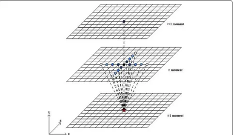
backward are reciprocal inverse process. Figure 1 is the 18-point (two orders in the time domain and eight orders in the space domain) format of RTM im-aging. The red pentagram on the t−1 moment plane

in Fig. 1 is the unsolved point which can be calcu-lated from the 17 points on the t moment plane and 1 point on the t+ 1 moment plane is needed as sup-port. The gradient color of the 17 points on the t

moment plane shows the degree of association for the unsolved point, and the darker the color, the greater the degree of association is; its value is determined by the difference coefficient.

(4)

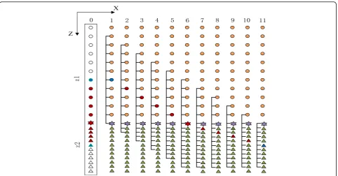
condition, it is found that the crux of the wave field value in the transitional zone is the number of the difference point of the 11 points on t time section of

Z direction. Figure 2 is the transitional zone of t time on (x,z) plane which is from high-velocity layer to low-velocity layer.

It can be seen from the Fig. 2 that the nine points of red color between Z1 and Z2 on zero line are the transitional zone, the small step length sampling in low-velocity layer which is represented by a triangle and two times of the small step in high-velocity layer which is represented by a circle, the hexagons are the velocity interface. It is supposed that each point in the X direction is at a consistent rate or a little change, so it takes sample with a fixed step length in the X direction, and it can use traditional RTM to compute the wave field values.

The multi-scale FDTD of forward wave field on transi-tional zone is shown as follows:

The first column has not entered the transition zone, the wave field value of the black point is shown in Eq. 3:

uki;‐j1¼2uki;jþuki;þj1 þV

2_Δ_t2

Δz2 fa5 u

k

i;jþ5þuki;j−5

h i

þa4 uki;jþ4þuki;j−4

h i

þa0uki;jg þ V2_Δ_t2

Δx2 X5

n¼1

g_k uk

iþn;jþuki−n;j−2uki;j

" #

ð3Þ

In which ai(i= 0, 1,⋯5) is the difference coefficient; the number of difference points on both sides of the der-ivation point is consistent.

The second column begins to enter the transition zone; the difference coefficient and the number of differ-ence point were changed because the step is unequal.Bz

in Eq.2which is at the position of the red point ont−1

time section is shown in Eq. 4, and bi(i= 0, 1,⋯, 5) is the difference coefficient:

Bz¼b5 uki;jþ6þuki;j−5

h i

þb4 uki;jþ4þuki;j−4

h i

þb1 uki;jþ1þu

k i;j−1

h i

þb0uki;j

ð4Þ

And then, the Bz of the red points in the transition zone from the third column to the fifth column are shown as follows:

Fig. 3The velocity model of the flat-layered model

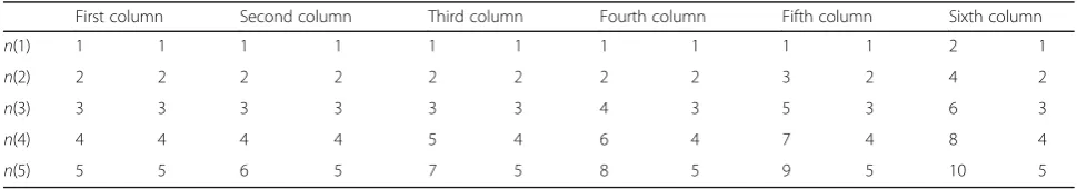
Table 1The value ofn(k) of 10 order FDTD

First column Second column Third column Fourth column Fifth column Sixth column

n(1) 1 1 1 1 1 1 1 1 1 1 2 1

n(2) 2 2 2 2 2 2 2 2 3 2 4 2

n(3) 3 3 3 3 3 3 4 3 5 3 6 3

n(4) 4 4 4 4 5 4 6 4 7 4 8 4

(5)

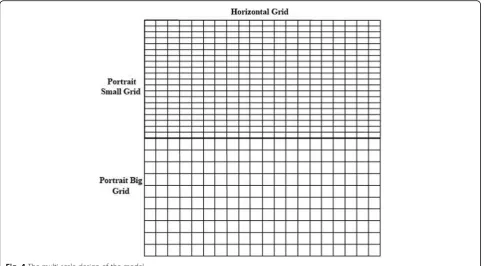
Fig. 4The multi-scale design of the model

(6)

Bz¼c5 uki;jþ7þuki;j−5

h i

þc4 uki;jþ5þuki;j−4

h i

þc3 uki;jþ3þu

k i;j−3

h i

þc2 uki;jþ2þu

k i;j−2

h i

þc0uki;j

ð5Þ

Bz¼d5 uki;jþ8þuki;j−5

h i

þd4 uki;jþ6þuki;j−4

h i

þd3 uki;jþ4þu

k i;j−3

h i

þd2 uki;jþ2þu

k i;j−2

h i

þd0uki;j

ð6Þ

Bz¼e5 uki;jþ9þuki;j−5

h i

þe4 uki;jþ7þuki;j−4

h i

þe0uki;j

ð7Þ

In which ci, di, ei(i= 0, 1,⋯, 5) are the difference coefficients.

The red hexagonal in the sixth column is on the vel-ocity interface, and Az is changed from this column. Based on the change of the grid step, theAzis shown in Eq.8andBzis shown in Eq.9.

Az¼ V 2_Δt

2 1 2Δz

2 ð8Þ

Fig. 6t= 30 ms snapshot of wave field of traditional method

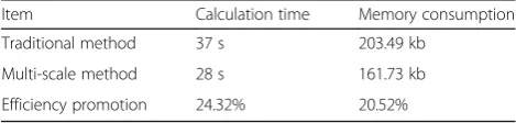
Table 2The comparison of calculation time and memory consumption between multi-scale method and traditional method

Item Calculation time Memory consumption

Traditional method 37 s 203.49 kb

Multi-scale method 28 s 161.73 kb

(7)

Bz¼a5 uki;jþ10þuki;j−5

h i

þa0uki;j

ð9Þ

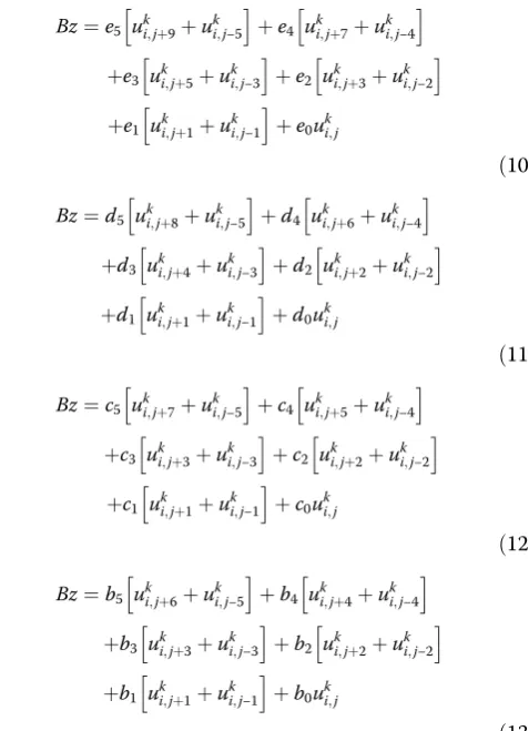
TheAzin Eq.8is employed from the seventh column to the tenth column, andBzare shown as follows:

Bz¼e5 uki;jþ9þuki;j−5

h i

þe3 uki;jþ5þu

k i;j−3

h i

þe2 uki;jþ3þu

k i;j−2

h i

þe0uki;j

ð10Þ

Bz¼d5 uki;jþ8þu

k i;j−5

h i

þd4 uki;jþ6þu

k i;j−4

h i

þd1 uki;jþ1þu

k i;j−1

h i

þd0uki;j

ð11Þ

Bz¼c5 uki;jþ7þu

k i;j−5

h i

þc4 uki;jþ5þu

k i;j−4

h i

þc1 uki;jþ1þu

k i;j−1

h i

þc0uki;j

ð12Þ

Bz¼b5 uki;jþ6þu

k i;j−5

h i

þb4 uki;jþ4þu

k i;j−4

h i

þb3 uki;jþ3þu

k i;j−3

h i

þb2 uki;jþ2þu

k i;j−2

h i

þb1 uki;jþ1þu

k i;j−1

h i

þb0uki;j

ð13Þ

It can be observed from the Eqs. 10–13 and Eqs.7–4 that the wave field formulas of points on the transition Fig. 8The multi-scale design of the model

(8)

zone are asymmetrical about the point of the velocity interface, and this law can be skillfully used in program-ming. At the same time, the variation of the difference points can be used as a new function for derivative for-mula ofZdirection; it is shown as follows:

∂2_U

∂z2 ¼

1

Δz2 XN

k¼1

mkUi;jþn kð Þ−2Ui;jþUi;j−n kð Þ ð14Þ

In which, mk is the difference coefficient which can be get from Taylor series, n(k) is the function of the differential point number. n(k) of the 10 order preci-sion finite difference is shown in Table 1. The differ-ence schemes of transition zone from low-velocity layer to high-velocity layer can be derived from the same reason and the difference scheme of X direction is as the same way.

3 Results and discussion

In general, it is too time-consuming to perform RTM imaging using a common personal computer (PC) and the efficiency is very low. In this paper, PC is used to

perform to demonstrate the feasibility and effectiveness of this method. The computer’s processor is Intel Core i5–7400, its memory is 8 GB, and the source is the rick wavelet of 30 Hz. The accuracy of the simulation is the 10 orders in space domain and 2 orders in time domain.

3.1 Flat-layered model

This is the two flat layers model; the size of the model is 100 m × 200 m, the velocity of the first layer is 1200 m/ s, the velocity of the second layer is 2400 m/s, and the velocity model is shown in Fig.3. The two scales of the grid are employed for this model, and the design idea is that thedx= 5manddz= 2.5mare used to the first layer which is the small step in Z direction, and the dx= 5m

and dz= 5m are used to the second layer which is the bigger step than the first layer inZdirection; the step of the X direction stays the same. The sketch map of the multi-scale design for this model is shown in Fig. 4. It should be noted that the grid of this model is from small to big, which velocity is from low to high, and the for-mula can be obtained by reverse recursion of Fig.2.

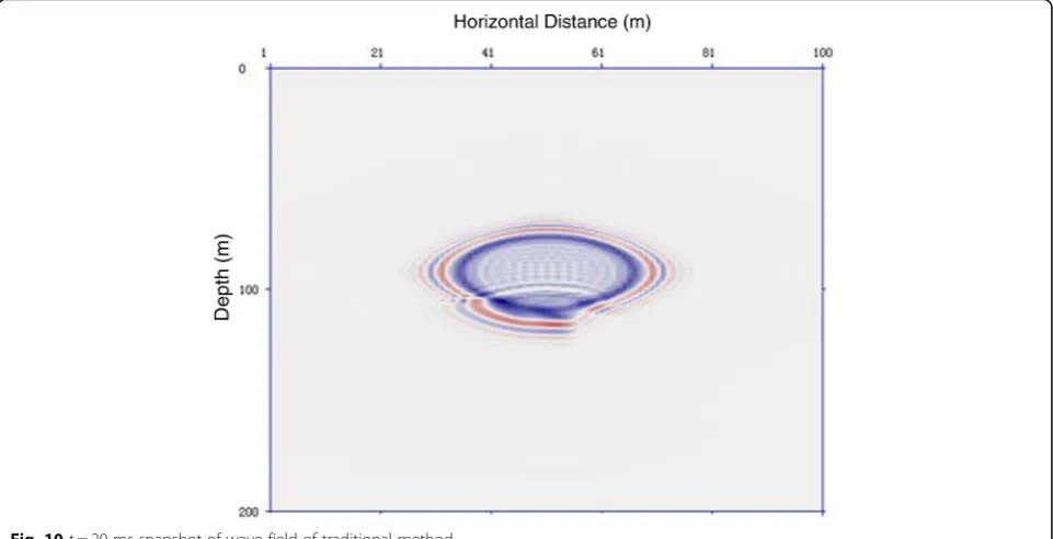
The wave field forward modeling is performed on the model, and the shot’s coordinates are 50 m and 75 m, the time interval is 0.5 ms, the snapshot of wave field when t= 30 ms used multi-scale method is shown in Fig.5, and in Fig.6is the result of traditional method. It can be seen from the two figures of the simulation results that the resolution of result based on the multi-scale method is the same as the traditional method; it can simulate the wave propagation well. Fig. 10t= 20 ms snapshot of wave field of traditional method

Table 3The comparison of calculation time and memory consumption between multi-scale method and traditional method

Traditional method 40s 203.49 kb

Multi-scale method 34 s 188.56 kb

(9)

Analysis from the perspective of comprehensive calcu-lation efficiency, the calcucalcu-lation time, and the memory consumption of the multi-scale method and the trad-itional method is shown in Table 2. It can be seen from Table 2 that the calculation time and the memory con-sumption are all shortened using multi-scale method, and the comprehensive calculation efficiency is im-proved. From the point of view of saving time, the multi-scale method improves efficiency by 24.32%.

3.2 Step model

There are two different velocity in the step model, and the size of the model is 100 m × 200 m, the velocity of the first layer is 1200 m/s, the velocity of the second layer is 2400 m/s, and the velocity model is shown in Fig. 7. It can be seen that there is a step in the model, and this model is to test and verify the applicability of multi-scale method for inflection. The coordinates of the step point are 57 and 110 m, and 57 and 125 m. The two scales of the grid is employed for this model, and the design idea is that the dx= 5m and dz= 2.5m are used to the first layer which is the small step inZ direc-tion, and the dx= 5m and dz= 5mare used to the sec-ond layer which is the bigger step than the first layer in

Z direction; the step of the X direction stays the same. The sketch map of the multi-scale design for this model is shown in Fig.8. It can be seen that the turning point of the step is in the yellow circle, and it is in the small-scale grid.

In this simulation, the coordinates of the shot are 50 and 75 m, and the time interval is 0.5 ms, the t= 20 ms snapshot of wave field used multi-scale method is shown in Fig. 9, and the result of traditional method is shown in Fig. 10. It can be seen from the result that the multi-scale method can simulate the wave propagation which agrees well with the theoretical. Analysis from the perspective of comprehensive calculation efficiency, the calculation time, and the memory consumption of the multi-scale method and the traditional method is shown in Table3. It can be seen from Table3 that the calcula-tion time and the memory consumpcalcula-tion are all short-ened using multi-scale method, and the integrated computing efficiency is improved. From the point of view of saving time, the multi-scale method improves ef-ficiency by 15%. It can be found that the efef-ficiency pro-motion is not the fixed value, and in this example, it is smaller than the above because of the velocity distribu-tion of the model; the bigger the area of the high vel-ocity, the higher the efficiency of the multi-scale method.

3.3 SEG/salt model

Salt model is developed by famous experts of Society of Exploration Geophysicists (SEG); the model has many highly difficult migration imaging challenges: large dip angle, many turning points, acute variety of velocity, and so on. The velocity model is shown in Fig.11, and it can be seen that there are many large dip angles which is ap-proaching 90 o. The presence of salt leads to the

(10)

Fig. 12The sketch map of the multi-scale design for salt model

(11)

emergence of multiple inflection points in small gaps which is the difficulty for migration imaging. And the imaging of the media beneath the salt body is also the challenge to migration.

The traditional RTM uses the fix step grid ofdx= 80ft,

dz= 80ft, nx= 1200, and nz= 150. In this paper, the multi-scale RTM is employed for salt model, and three different scales are used to salt model according to the characteristics of the velocity model. The sketch map of the multi-scale design for this model is shown in Fig.12, and it needs to be pointed out that the Fig.12 only shows multi-scale partitioning but not the real number of the grid. It can be seen from Fig. 12 that the most salt body which is the high-velocity area and its velocity is 14,700 m/s; this area is in the green frame which uses the grid ofdx= 320ft anddz= 320ft, which is the big step grid, and the edge of the salt body are almost in small step grid because the edge needs precise imaging. The area in the yellow frame uses the grid ofdx= 160ft and dz= 160ft; it is the medium velocity zone, and the other area of the salt model uses the original scale ofdx= 80ft anddz= 80ft. It needs to point that the big scale is an even multiple of small scales which is in accordance with the velocity model in this paper. In general, the relationship of the two velocities is an even number of times the scale of them is also an even multiple, if they are not an even multiple for

each other, it can choose the minimum even which is big-ger than real multiple. In this example, the velocity of the blue area is 14,700 m/s, and the minimum velocity is 5000 m/s which is in the red area; the high velocity is al-most three times low, so the four times is chosen for the big scale. The light blue area uses twice the scale.

The result of multi-scale RTM is shown in Fig.13; it can be seen that the area in the green frame is imaged clearly which is the interior of the salt body that used four times the scale, the area in the yellow circle is medium velocity zone which uses two times the scale, and its imaging is clear. And the areas in the red circles are the minor faults beneath the salt body; they are also imaged well and not affected by the four times scale of the salt body. The scale-three traditional RTM result is shown in Fig.14and it uses the scale-three on the whole salt model; compared with Fig.13, it can be seen that the areas in the red circle Fig. 14The result of scale-three RTM

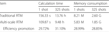
Table 4The comparison between multi-scale RTM and traditional RTM

1 shot 325 shots 1 shots 325 shots

Traditional RTM 156.33 s 13.76 h 8.21 M 2.60 G

Multi-scale RTM 109.87 s 9.48 h 5.83 M 1.85 G

(12)

and rectangle have lower resolution, so the precision of multi-scale RTM is better than the traditional RTM. The reason that the multi-scale RTM is very flexible to the geologic model which can use the bigger scale on higher-velocity area and the smaller scale on the lower velocity area for one geologic model, so the algorithm can get the balance between the precision and efficiency, and it can select the best one from the precision and efficiency, which is the best precision in the same efficiency and the highest efficiency in the same precision.

Table 4 is the comparison of calculation time and memory consumption between multi-scale RTM and traditional RTM. It can be observed from Table 4 that the multi-scale RTM is better than traditional RTM whether in calculation time and memory consumption, and the migration imaging is clear.

4 Conclusions

The paper has tested and verified that the multi-scale RTM can improve the integrated computing efficiency though the different examples, and it has improved the calculation efficiency by 25.05% average within the paper.

The multi-scale RTM is an effective method for im-proving computational efficiency, it has three character-istics to traditional RTM as follows: (1) it uses the big scale grid for high-velocity area to reduce the calculated amount which can improve the computational efficiency; (2) it uses scale grid for deep low speed interlayer to im-prove imaging accuracy; (3) it does not need to interpolate in the transition zone which can avoid the accumulation of errors caused by interpolation. In con-clusion, the multi-scale RTM has the characteristics of high efficiency and precision, it lays the foundation for RTM application in practice, and the experimental re-sults show that the algorithm is effective and reliable.

Abbreviations

FDTD:Finite difference time domain; GPU: Graphics processing unit; PC: Personal computer; RTM: Reverse time migration; SGE: Society of Exploration Geophysicists

Acknowledgements

The authors thank the editor and anonymous reviewers for their helpful comments and valuable suggestions.

Funding

The research work was supported in part by a grant from the Natural Science Foundation of China (no. 61401347), a grant from Natural Science Foundation of Shaanxi Province Department of Education of China under Grant No. 16JK1322; Xi’an Polytechnic University Doctor Scientific Research foundation of China under Grant No. BS1118.

Availability of data and materials

We can provide the data.

Authors_’contributions

All authors took part in the discussion of the work described in this paper. XZ wrote the first version of the paper. LZ carried out the experiments of the paper. HG revised the paper in different version. The contributions of the proposed work are mainly in two aspects: (1) to the best of our knowledge, our work is the first one to apply the multi-scale idea for RTM imaging based

on FDTD. Without any interpolation to the transitional zone, our method just deduce the wave equation though the Taylor series of mathematical method. (2) The novelty of our method attributes to the use of RTM imaging to preserve imaging accuracy while improving the integrated computing ef-ficiency and refining the precision of the imaging area. All authors read and approved the final manuscript.

Authors’information

Xiaodan Zhang received the B.S. degree in communication engineering from Xi‘an Communication College, Xi’an, China, in 2004, the MS degree in circuit and system from Xi_’an University of Technology, Xi_’an, China, in 2008, and the Ph.D degree in Microelectronics and Solid-State Electronics from Xi’an University of Technology, Xi_’an, China, in 2012. In 2011, She joined Xi_’an Poly-technic University, Xi’an, China. From 2011 to present, she was a lecturer in the College of Electronic and Information at Xi_’an Polytechnic University. Since September 2017, she joined Xi‘an Jiaotong University as a young back-bone visiting scholar. Her research interests include migration imaging, im-aging signal processing, and wavelet analysis.

Lei Zhu received his B. S. and M. S. degrees form communication engineering, Xi’an Polytechnic University in 2002 and 2005, respectively, and Ph.D degree in signal and information processing in Xidian University in 2012. He is a Professor at the college of Electronic and Information, Xi’an University of Technology. His current research interests include SAR image processing, computer vision.

Hua Guo received his B. S. degree in applied physics frOm Xidian University in 2004, and M. S. degrees in radio physics from Xidian University in 2007, and the Ph.D. degree in electromagnetic field and microwave technology from Northwestern Polytechnical University in 2015. He is a lecturer in the college of electronic and information at Xi_’an Polytechnic University. His current research interests include array signal processing, image processing, and machine learning.

Competing interests

There are no potential competing interests in our paper.

Publisher’s Note

Springer Nature remains neutral with regard to jurisdictional claims in published maps and institutional affiliations.

Received: 11 April 2018 Accepted: 13 June 2018

References

1. Z Li, X Li, J Xiao, B Hu, Amplitude-preserved reverse time migration with Gaussian beam based on crosscorrelation imaging conditions. Comput Tech Geophys Geochem Explor39, 354–358 (2017)

2. E Baysal, DD Kosloff, JWC Sherwood, Reverse time migration. Geophysics48, 1514–1524 (1983)

3. H Guan, E Dussaud, B Denel, P Williamson, inSEG 81st Annual International Meeting: September 18–23, 2011; San Antonio, USA. Techniques for an efficient implementation of RTM in TTI media (2011), pp. 3393–3397 4. W Dai, P Fowler, GT Schuster, Multisource least-squares reverse-time

migration. Geophys. Prospect.60, 681_–695 (2012)

5. H Wen, D Zhang, X Zheng, S Fan, W Wang, Propagation characteristics of electromagnetic wave based on FDTD in coal. J. China Coal Soc.42, 2959– 2967 (2017)

6. Y Zhang, L Duang, Y Xie, inSEG 83rd Annual International Meeting: September 22–27, 2013; Houston, USA. A stable and practical implementation of least-squares reverse time migration (2013), pp. 3716–3720

7. Y Liu, WW Symes, Z Li, inSEG 83rd Annual International Meeting: September 22_–27, 2013; Houston, USA. Multisource least-squares extended reverse-time migration with preconditioning guided gradient method (2013), p. 1251 8. DC Del Rey Fernandez, JE Hicken, DW Zingg, Review of summation-by-parts

operators with simultaneous approximation terms for the numerical solution of partial differential equations. J. Sci. Comput.95, 171_–196 (2014) 9. B Sjögreen, High order finite difference and finite volume methods for

advection on the sphere. J. Sci. Comput.51, 703–732 (2014)

(13)

11. Y Rao, YH Wang, Seismic waveform simulation with pseudo-orthogonal grids for irregular topographic models. Geophys. J. Int. 194, 1778–1788 (2013)

12. B LI, HW LIU, GF LIU, Computational strategy of seismic pre-stack reverse time migration on CPU/GPU. Chin. J. Geophys.53, 2938–2943 (2010) 13. WG Wang, SJ Xiong, HN Xu, RY Qian, TTI media anisotropic

pseudo-spectral method inverse time migration. Pet Geophys Explor47, 566– 572+682+513 (2012)

14. JE Kozdon, EM Dunham, J Nordstrom, Simulation of dynamic earthquake ruptures in complex geometries using high-order finite difference methods. J. Sci. Comput.55, 92–124 (2013)

15. JP Huang, Q Zhang, K Zhang, ZC Li, YB Yue, ML Yuan, Green function gaussian beam inverse time deviation. Pet Geophys Explor49, 101–106+303 (2014)

16. B Wang, J Gao, W Cheng, H Zhang, Efficient boundary storages strategies for seismic inverse time migration. Chin. J. Geophys.55, 2412–2421 (2012) 17. H Zhao, J Gao, Y Ma, An absorbing boundary algorithm for diffusive-viscous

wave equation. J. Xi'an Jiaotong Univ.46, 112_–118 (2012)

18. W Meng, L-Y Fu, Seismic wavefield simulation by a modified finite element method with a perfectly matched layer absorbing boundary. J. Geophys. Eng.14, 852 (2017)

19. L Na, Multi-source least-squares inverse time migration based on Huber norm. Pet Geophys Explor52, 941–947+878 (2017)