DOI10.1186/2190-8567-1-4
R E S E A R C H Open Access
Analysis of a hyperbolic geometric model for visual
texture perception
Grégory Faye·Pascal Chossat·Olivier Faugeras
Received: 7 January 2011 / Accepted: 6 June 2011 / Published online: 6 June 2011
© 2011 Faye et al.; licensee Springer. This is an Open Access article distributed under the terms of the Creative Commons Attribution License
Abstract We study the neural field equations introduced by Chossat and Faugeras to model the representation and the processing of image edges and textures in the hy-percolumns of the cortical area V1. The key entity, the structure tensor, intrinsically lives in a non-Euclidean, in effect hyperbolic, space. Its spatio-temporal behaviour is governed by nonlinear integro-differential equations defined on the Poincaré disc model of the two-dimensional hyperbolic space. Using methods from the theory of functional analysis we show the existence and uniqueness of a solution of these equa-tions. In the case of stationary, that is, time independent, solutions we perform a sta-bility analysis which yields important results on their behavior. We also present an original study, based on non-Euclidean, hyperbolic, analysis, of a spatially localised bump solution in a limiting case. We illustrate our theoretical results with numerical simulations.
Keywords Neural fields·nonlinear integro-differential equations·functional analysis·non-Euclidean analysis·stability analysis·hyperbolic geometry· hypergeometric functions·bumps
Mathematics Subject Classification 30F45·33C05·34A12·34D20·34D23· 34G20·37M05·43A85·44A35·45G10·51M10·92B20·92C20
G Faye (
)·P Chossat·O FaugerasNeuroMathComp Laboratory, INRIA, Sophia Antipolis, CNRS, ENS Paris, Paris, France e-mail:[email protected]
P Chossat
1 Introduction
The selectivity of the responses of individual neurons to external features is often the basis of neuronal representations of the external world. For example, neurons in the primary visual cortex (V1) respond preferentially to visual stimuli that have a specific orientation [1–3], spatial frequency [4], velocity and direction of motion [5], color [6]. A local network in the primary visual cortex, roughly 1 mm2of cortical surface, is assumed to consist of subgroups of inhibitory and excitatory neurons each of which is tuned to a particular feature of an external stimulus. These subgroups are the so-called Hubel and Wiesel hypercolumns of V1. We have introduced in [7] a new approach to model the processing of image edges and textures in the hypercolumns of area V1 that is based on a nonlinear representation of the image first order derivatives called the structure tensor [8,9]. We suggested that this structure tensor was represented by neuronal populations in the hypercolumns of V1. We also suggested that the time evolution of this representation was governed by equations similar to those proposed by Wilson and Cowan [10]. The question of whether some populations of neurons in V1 can represent the structure tensor is discussed in [7] but cannot be answered in a definite manner. Nevertheless, we hope that the predictions of the theory we are developing will help deciding on this issue.
Our present investigations were motivated by the work of Bressloff, Cowan, Gol-ubitsky, Thomas and Wiener [11,12] on the spontaneous occurence of hallucinatory patterns under the influence of psychotropic drugs, and its extension to the structure tensor model. A further motivation was the following studies of Bressloff and Cowan [4,13,14] where they study a spatial extension of the ring model of orientation of Ben-Yishai [1] and Hansel, Sompolinsky [2]. To achieve this goal, we first have to better understand the local model, that is the model of a ‘texture’ hypercolumn iso-lated from its neighbours.
2 The model
By definition, the structure tensor is based on the spatial derivatives of an image in a small area that can be thought of as part of a receptive field. These spatial derivatives are then summed nonlinearly over the receptive field. LetI (x, y)denote the original image intensity function, wherex andy are two spatial coordinates. LetIσ1 denote the scale-space representation ofIobtained by convolution with the Gaussian kernel
gσ(x, y)=21 π σ2e−(x
2+y2)/(2σ2) :
Iσ1=I g
σ1.
The gradient∇Iσ1 is a two-dimensional vector of coordinatesIσ1
x ,Iyσ1 which
em-phasizes image edges. One then forms the 2×2 symmetric matrix of rank one
T0= ∇Iσ1(∇Iσ1)T, whereTindicates the transpose of a vector. The set of 2×2 sym-metric positive semidefinite matrices of rank one will be noted S+(1,2)throughout the paper (see [16] for a complete study of the set S+(p, n)ofn×nsymmetric pos-itive semidefinite matrices of fixed-rankp < n). By convolvingT0componentwise with a Gaussiangσ2 we finally form the tensor structure as the symmetric matrix:
T =T0 gσ2=
(Iσ1
x )2σ2 I
σ1
x Iyσ1σ2
Iσ1
x Iyσ1σ2 (I
σ1
y )2σ2
,
where we have set for example:
Iσ1
x
2
σ2=
Iσ1
x
2
gσ2.
Since the computation of derivatives usually involves a stage of scale-space smoothing, the definition of the structure tensor requires two scale parameters. The first one, defined byσ1, is a local scale for smoothing prior to the computation of image derivatives. The structure tensor is insensitive to noise and details at scales smaller thanσ1. The second one, defined byσ2, is an integration scale for accumu-lating the nonlinear operations on the derivatives into an integrated image descriptor. It is related to the characteristic size of the texture to be represented, and to the size of the receptive fields of the neurons that may represent the structure tensor.
By construction,T is symmetric and non negative as det(T)≥0 by the inequal-ity of Cauchy-Schwarz, then it has two orthonormal eigenvectorse1,e2and two non negative corresponding eigenvaluesλ1 andλ2 which we can always assume to be such thatλ1≥λ2≥0. Furthermore the spatial averaging distributes the information of the image over a neighborhood, and therefore the two eigenvalues are always pos-itive. Thus, the set of the structure tensors lives in the set of 2×2 symmetric positive definite matrices, noted SPD(2,R)throughout the paper. The distribution of these eigenvalues in the(λ1, λ2)plane reflects the local organization of the image intensity variations. Indeed, each structure tensor can be written as the linear combination:
T =λ1e1eT1 +λ2e2eT2=(λ1−λ2)e1eT1+λ2
e1eT1 +e2eT2
=(λ1−λ2)e1eT1+λ2I2,
whereI2is the identity matrix ande1eT1∈S+(1,2). Some easy interpretations can be made for simple examples: constant areas are characterized byλ1=λ2≈0, straight edges are such that λ1λ2≈0, their orientation being that of e2, corners yield
λ1≥λ20. The coherencycof the local image is measured by the ratioc=λλ1−1+λλ22, large coherency reveals anisotropy in the texture.
We assume that a hypercolumn of V1 can represent the structure tensor in the re-ceptive field of its neurons as the average membrane potential values of some of its membrane populations. LetT be a structure tensor. The time evolution of the average potentialV (T, t )for a given column is governed by the following neural mass equa-tion adapted from [7] where we allow the connectivity functionW to depend upon the time variabletand we integrate over the set of 2×2 symmetric definite-positive matrices:
⎧ ⎪ ⎪ ⎨ ⎪ ⎪ ⎩
∂tV (T, t )= −αV (T, t )+
SPD(2)
W (T,T , t )SV (T , t )dT
+Iext(T, t ) ∀t >0,
V (T,0)=V0(T).
(2)
The nonlinearitySis a sigmoidal function which may be expressed as:
S(x)= 1
1+e−μx,
whereμdescribes the stiffness of the sigmoid.Iextis an external input.
The set SPD(2) can be seen as a foliated manifold by way of the set of spe-cial symmetric positive definite matrices SSPD(2)=SPD(2)∩SL(2,R). Indeed, we have: SPD(2)hom= SSPD(2)×R+∗. Furthermore, SSPD(2)isom= D, whereDis the Poincaré Disk, see, for example, [7]. As a consequence we use the following folia-tion of SPD(2): SPD(2)hom= D×R+∗, which allows us to write for allT ∈SPD(2),
T =(z, )with(z, )∈D×R+∗.T,zandare related by the relation det(T)=2
and the fact thatzis the representation inDofT˜ ∈SSPD(2)withT =T˜. It is well-known [17] thatD(and hence SSPD(2)) is a two-dimensional Rieman-nian space of constant sectional curvature equal to−1 for the distance notedd2 de-fined by
d2(z, z)=arctanh |
z−z|
|1− ¯zz|.
The isometries ofD, that are the transformations that preserve the distanced2are the elements of unitary group U(1,1). In AppendixAwe describe the basic structure of this group. It follows, for example, [7, 18], that SDP(2) is a three-dimensional Riemannian space of constant sectional curvature equal to−1 for the distance noted
d0defined by
d0(T,T )=
As shown in PropositionB.0.1of AppendixBit is possible to express the volume elementdT in(z1, z2, )coordinates withz=z1+iz2:
dT =8√2d
dz1dz2
(1− |z|2)2. We note dm(z)= dz1dz2
(1−|z|2)2 and equation (2) can be written in(z, )coordinates:
∂tV (z, , t )= −αV (z, , t )
+8√2
+∞
0
DW
z, , z, , tSV (z, , t )d
dm(z)
+Iext(z, , t ).
We get rid of the constant 8√2 by redefiningWas 8√2W.
⎧ ⎪ ⎪ ⎪ ⎪ ⎪ ⎨ ⎪ ⎪ ⎪ ⎪ ⎪ ⎩
∂tV (z, , t )= −αV (z, , t )
+ +∞
0
DW (z, , z, , t )S
V (z, , t )d
dm(z)
+Iext(z, , t ) ∀t >0,
V (z, ,0)=V0(z, ).
(3)
In [7], we have assumed that the representation of the local image orientations and textures is richer than, and contains, the local image orientations model which is conceptually equivalent to the direction of the local image intensity gradient. The richness of the structure tensor model has been expounded in [7]. The embedding of the ring model of orientation in the structure tensor model can be explained by the intrinsic relation that exists between the two sets of matrices SPD(2,R) and S+(1,2). First of all, when σ2goes to zero, that is when the characteristic size of the structure becomes very small, we haveT0 gσ2→T0, which means that the ten-sorT ∈SPD(2,R)degenerates to a tensorT0∈S+(1,2), which can be interpreted as the loss of one dimension. We can write eachT0∈S+(1,2)asT0=xxT=r2uuT, whereu=(cosθ,sinθ )Tand(r, θ )is the polar representation ofx. Since,xand−x
correspond to the sameT0,θis equated toθ+kπ,k∈Z. Thus S+(1,2)=R+∗ ×P1, whereP1 is the real projective space of dimension 1 (lines of R2). Then the inte-gration scaleσ2, at which the averages of the estimates of the image derivatives are computed, is the link between the classical representation of the local image ori-entations by the gradient and the representation of the local image textures by the structure tensor. It is also possible to highlight this explanation by coming back to the interpretation of straight edges of the previous paragraph. Whenλ1λ2≈0 then
T ≈(λ1−λ2)e1eT1 ∈S+(1,2)and the orientation is that ofe2. We denote byPthe projection of a 2×2 symmetric definite positive matrix on the set S+(1,2)defined by:
P:
whereT is as in equation (1). We can introduce a metric on the set S+(1,2)which is derived from a well-chosen Riemannian quotient geometry (see [16]). The resulting Riemannian space has strong geometrical properties: it is geodesically complete and the metric is invariant with respect to all transformations that preserve angles (orthog-onal transformations, scalings and pseudoinversions). Related to the decomposition S+(1,2)=R+∗ ×P1, a metric on the space S+(1,2)is given by:
ds2=2
dr r
2
+dθ2.
The space S+(1,2)endowed with this metric is a Riemannian manifold (see [16]). Finally, the distance associated to this metric is given by:
dS2+(1,2)(τ1, τ2)=2 log
2
r1
r2
+ |θ1−θ2|2,
whereτ1=x1Tx1,τ2=x2Tx2and(ri, θi)denotes the polar coordinates ofxi fori=
1,2. The volume element in(r, θ )coordinates is:
dτ=dr
r dθ
π ,
where we normalize to 1 the volume element for theθcoordinate.
Let nowτ=P(T)be a symmetric positive semidefinite matrix. The average po-tentialV (τ, t )of the column has its time evolution that is governed by the follow-ing neural mass equation which is just a projection of equation (2) on the subspace S+(1,2):
∂tV (τ, t )= −αV (τ, t )+
S+(1,2)
W (τ, τ, t )SV (τ , t )dτ
+Iext(τ, t ) ∀t >0.
(4)
In(r, θ )coordinates, (4) is rewritten as:
∂tV (r, θ, t )= −αV (r, θ, t )+
+∞
0
π
0
W (r, θ, r, θ, t )SV (r, θ, t )dθ π
dr r
+Iext(r, θ, t ).
This equation is richer than the ring model of orientation as it contains an ad-ditional information on the contrast of the image in the orthogonal direction of the prefered orientation. If one wants to recover the ring model of orientation tuning in the visual cortex as it has been presented and studied by [1,2,19], it is sufficient i) to assume that the connectivity function is time-independent and has a convolutional form:
W (τ, τ , t )=wdS+(1,2)(τ, τ)
=w
2 log2
r r
+ |θ−θ|2
and ii) to look at semi-homogeneous solutions of equation (4), that is, solutions which do not depend upon the variabler. We finally obtain:
∂tV (θ, t )= −αV (θ, t )+
π
0
wsh(θ−θ)SV (θ, t )dθ
π +Iext(θ, t ), (5)
where:
wsh(θ )=
+∞
0
w2 log2(r)+θ2dr
r .
It follows from the above discussion that the structure tensor contains, at a given scale, more information than the local image intensity gradient at the same scale and that it is possible to recover the ring model of orientations from the structure tensor model.
The aim of the following sections is to establish that (3) is well-defined and to give necessary and sufficient conditions on the different parameters in order to prove some results on the existence and uniqueness of a solution of (3).
3 The existence and uniqueness of a solution
In this section we provide theoretical and general results of existence and uniqueness of a solution of (2). In the first subsection (Section3.1) we study the simpler case of the homogeneous solutions of (2), that is, of the solutions that are independent of the tensor variableT. This simplified model allows us to introduce some notations for the general case and to establish the useful Lemma3.1.1. We then prove in Section3.2
the main result of this section, that is the existence and uniqueness of a solution of (2). Finally we develop the useful case of the semi-homogeneous solutions of (2), that is, of solutions that depend on the tensor variable but only through itszcoordinate inD.
3.1 Homogeneous solutions
A homogeneous solution to (2) is a solutionV that does not depend upon the tensor variableT for a given homogenous inputI (t )and a constant initial conditionV0. In
(z, )coordinates, a homogeneous solution of (3) is defined by:
˙
V (t )= −αV (t )+W (z, , t )SV (t )+Iext(t ), where:
W (z, , t )def=
+∞
0
DW (z, , z, , t )
d
dz1dz2
(1− |z|2)2. (6)
Hence necessary conditions for the existence of a homogeneous solution are that:
• the double integral (6) is convergent,
• W (z, , t )does not depend upon the variable(z, ). In that case, we writeW (t )
In the special case whereW (z, , z, , t )is a function of only the distanced0 between(z, )and(z, ):
W (z, , z, , t )≡w2(log−log)2+d2 2(z, z), t
the second condition is automatically satisfied. The proof of this fact is given in LemmaD.0.2of AppendixD. To summarize, the homogeneous solutions satisfy the differential equation:
˙
V (t )= −αV (t )+W (t )SV (t )+Iext(t ), t >0,
V (0)=V0.
(7)
3.1.1 A first existence and uniqueness result
Equation (3) defines a Cauchy’s problem and we have the following theorem.
Theorem 3.1.1 If the external inputIext(t )and the connectivity functionW (t )are continuous on some closed intervalJ containing0,then for allV0inR,there exists a unique solution of (7) defined on a subinterval J0 of J containing 0 such that
V (0)=V0.
Proof It is a direct application of Cauchy’s theorem on differential equations. We consider the mappingf :J×R→Rdefined by:
f (t, x)= −αx+W (t )S(x)+Iext(t ).
It is clear thatf is continuous fromJ×RtoR. We have for allx, y∈Randt∈J:
f (t, x)−f (t, y)≤α|x−y| +W (t )Sm|x−y|,
whereSm=supx∈R|S(x)|.
Since,W is continuous on the compact intervalJ, it is bounded there byC >0 and:
f (t, x)−f (t, y)≤(α+CSm)|x−y|.
We can extend this result to the whole time real line ifI andW are continuous onR.
Proposition 3.1.1 IfIextandW are continuous onR+,then for allV0 inR,there exists a unique solution of(7)defined onR+such thatV (0)=V0.
Proof We have already shown the following inequality:
f (t, x)−f (t, y)≤α|x−y| +W (t )Sm|x−y|.
Then we have for allt≥0:
V (t )=e−αtV0+
t
0
e−α(t−u)W (u)SV (u)du+
t
0
e−α(t−u)Iext(u) du
⇒ V (t )≤ |V0| +Sm
β
0
eαuW (u)du+
β
0
eαuIext(u)du ∀t∈ [0, β],
whereSm=supx∈R|S(x)|.
This implies that the maximal solutionV is bounded for allt∈ [0, β], but Theo-remC.0.2of AppendixCensures that it is impossible. Then, it follows that
necessar-ilyβ= +∞.
3.1.2 Simplification of(6)in a special case
Invariance In the previous section, we have stated that in the special case where
W was a function of the distance between two points inD×R+∗, thenW (z, , t )
did not depend upon the variables(z, ). As already said in the previous section, the following result holds (see proof of LemmaD.0.2of AppendixD).
Lemma 3.1.1 Suppose thatW is a function of d0(T,T )only. ThenW does not depend upon the variableT.
Mexican hat connectivity In this paragraph, we push further the computation ofW
in the special case whereW does not depend upon the time variablet and takes the special form suggested by Amari in [20], commonly referred to as the ‘Mexican hat’ connectivity. It features center excitation and surround inhibition which is an effective model for a mixed population of interacting inhibitory and excitatory neurons with typical cortical connections. It is also only a function ofd0(T,T ).
In detail, we have:
W (z, , z)=w2(log−log)2+d2
2(z, z)
,
where:
w(x)= 1
2π σ12 e−
x2 σ2
1 − A 2π σ22
e−
x2 σ2 2
with 0≤σ1≤σ2and 0≤A≤1.
In this case we can obtain a very simple closed-form formula forW as shown in the following lemma.
Lemma 3.1.2 WhenWis the specific Mexican hat function just defined then:
W=π
3 2
2
σ1e2σ 2
whereerf is the error function defined as:
erf(x)=√2 π
x
0
e−u2du.
Proof The proof is given in LemmaE.0.3of AppendixE.
3.2 General solution
We now present the main result of this section about the existence and uniqueness of solutions of equation (2). We first introduce some hypotheses on the connectivity functionW. We present them in two ways: first on the set of structure tensors con-sidered as the set SPD(2), then on the set of tensors seen asD×R+∗. Let J be a subinterval ofR. We assume that:
• (H1):∀(T,T , t )∈SPD(2)×SPD(2)×J,W (T,T , t )≡W (d0(T,T ), t ),
• (H2):W∈C(J, L1(SPD(2)))whereWis defined asW(T, t )=W (d0(T,Id2), t ) for all(T, t )∈SPD(2)×J where Id2is the identity matrix ofM2(R),
• (H3): ∀t ∈ J, supt∈JW(t )L1 <+∞ where W(t )L1
def
= SPD(2)|W (d0(T, Id2), t )|dT.
Equivalently, we can express these hypotheses in(z, )coordinates:
• (H1bis):∀(z, z, , , t )∈D2×(R∗+)2×R, W (z, , z, , t )≡W (d2(z, z),
|log()−log()|, t ),
• (H2bis):W∈C(J, L1(D×R+∗))whereWis defined asW(z, , t )=W (d2(z,0),
|log()|, t )for all∀(z, , t )∈D×R+∗ ×J,
• (H3bis):∀t∈J, supt∈JW(t )L1<+∞where
W(t ) L1
def =
D×R+ ∗
Wd2(z,0),log(), t
d
dm(z).
3.2.1 Functional space setting
We introduce the following mappingfg:(t, φ)→fg(t, φ)such that:
fg(t, φ)(z, )=
D×R+∗
W
d2(z, z),
log
, t
Sφ (z, )d
dm(z). (9)
Our aim is to find a functional spaceFwhere (3) is well-defined and the function
fg mapsF toF for allts. A natural choice would be to choose φ as a Lp(D×
R+
∗)-integrable function of the space variable with 1≤p <+∞. Unfortunately, the homogeneous solutions (constant with respect to(z, )) do not belong to that space. Moreover, a valid model of neural networks should only produce bounded membrane potentials. That is why we focus our choice on the functional spaceF=L∞(D×
R+
Proposition 3.2.1 IfIext∈C(J,F)withsupt∈JIext(t )F <+∞ andW satisfies hypotheses(H1bis)-(H3bis)thenfgis well-defined and is fromJ×FtoF. Proof ∀(z, , t )∈D×R+∗ ×R, we have:
D×R+
∗
W
d2(z, z),
log , t
Sφ (z, )d
dm(z)
≤Smsup
t∈J
W(t )
L1<+∞.
3.2.2 The existence and uniqueness of a solution of (3)
We rewrite (3) as a Cauchy problem:
⎧ ⎪ ⎪ ⎪ ⎪ ⎪ ⎪ ⎪ ⎪ ⎪ ⎨ ⎪ ⎪ ⎪ ⎪ ⎪ ⎪ ⎪ ⎪ ⎪ ⎩
∂tV (z, , t )= −αV (z, , t )
+
D×R+∗
W
d2(z, z),
log , t
×SV (z, , t )d
dm(z)
+Iext(z, , t ),
V (z, ,0)=V0(z, ).
(10)
Theorem 3.2.1 If the external currentIextbelongs toC(J,F)withJan open interval containing0and W satisfies hypotheses(H1bis)-(H3bis),then fo allV0∈F,there exists a unique solution of (10)defined on a subinterval J0 ofJ containing0 such thatV (z, ,0)=V0(z, )for all(z, )∈D×R+∗.
Proof We prove thatfgis continuous onJ×F. We have
fg(t, φ)−fg(s, ψ )(z, )
=
D×R+ ∗
W
d2(z, z),
log
, tSφ (z, )−Sψ (z, )d
dm(z)
+
D×R+∗
W
d2(z, z),
log , t −W
d2(z, z),
log , s
×Sψ (z, )d
dm(z),
and therefore
fg(t, φ)−fg(s, ψ )F≤Smsup
t∈J
W(t )L1φ−ψF+SmW(t )−W(s)L1.
Because of condition (H2) we can choose |t −s| small enough so thatW(t )−
W(s)L1 is arbitrarily small. This proves the continuity offg. Moreover it follows from the previous inequality that:
with W0g =supt∈JW(t )L1. This ensures the Lipschitz continuity of fg with respect to its second argument, uniformly with respect to the first. The Cauchy-Lipschitz theorem on a Banach space yields the conclusion.
Remark 3.2.1 Our result is quite similar to those obtained by Potthast and Graben in[21].The main differences are that,first,we allow the connectivity function to depend upon the time variablet and,second,that our space features is no longer a
Rnbut a Riemanian manifold.In their article,Potthast and Graben also work with a
different functional space by assuming more regularity for the connectivity function
Wand then obtain more regularity for their solutions.
Proposition 3.2.2 If the external current Iextbelongs toC(R+,F)andW satisfies hypotheses(H1bis)-(H3bis)withJ =R+,then for allV0∈F,there exists a unique solution of(10)defined onR+such thatV (z, ,0)=V0(z, )for all(z, )∈D×
R+ ∗.
Proof We have just seen in the previous proof thatfg is globally Lipschitz with respect to its second argument:
fg(t, φ)−fg(t, ψ )F≤SmW0gφ−ψF
then TheoremC.0.3of AppendixCgives the conclusion.
3.2.3 The intrinsic boundedness of a solution of (3)
In the same way as in the homogeneous case, we show a result on the boundedness of a solution of (3).
Proposition 3.2.3 If the external currentIextbelongs toC(R+,F)and is bounded in timesupt∈R+Iext(t )F<+∞andW satisfies hypotheses(H1bis)-(H3bis)with
J=R+,then the solution of (10)is bounded for each initial conditionV0∈F. Let us set:
ρgdef= 2 α
SmW0g+ sup
t∈R+
Iext(t )F
,
whereW0g=supt∈R+W(t )L1.
Proof LetV be a solution defined onR+. Then we have for allt∈R+∗:
V (z, , t )=e−αtV0(z, )+
t
0
e−α(t−u)
D×R+∗
W
d2(z, z),
log
, u
×SV (z, , u)d
dm(z) du
+ t
0
The following upperbound holds
V (t )F≤e−αtV0F+ 1
α
SmW0g+ sup
t∈R+
Iext(t )F
1−e−αt. (11)
We can rewrite (11) as:
V (t )F≤e−αt
V0F− 1
α
SmW0g+sup
t∈R+
Iext(t )F
+ 1
α
SmW0+g sup
t∈R+
Iext(t )F
=e−αt
V0F−
ρg
2
+ρg
2 .
(12)
IfV0∈Bρgthis impliesV (t )F≤ρ
g
2(1+e−αt)for allt >0 and henceV (t )F<
ρg for allt >0, proving thatBρ is stable. Now assume thatV (t )F > ρg for all t≥0. The inequality (12) shows that fort large enough this yields a contradiction. Therefore there existst0>0 such thatV (t0)F=ρg. At this time instant we have
ρg≤e−αt0
V0F−
ρg
2
+ρg
2 , and hence
t0≤ 1
αlog
2V0F−ρg
ρg
.
The following corollary is a consequence of the previous proposition.
Corollary 3.2.1 IfV0∈/BρgandTg=inf{t >0such thatV (t )∈Bρg}then:
Tg≤ 1
αlog
2V0F−ρg
ρg
.
3.3 Semi-homogeneous solutions
solutions:
⎧ ⎪ ⎪ ⎨ ⎪ ⎪ ⎩
∂tV (z, t )= −αV (z, t )+
DW
sh(z, z, t )SV (z, t )
dm(z)
+Iext(z, t ), t >0,
V (z,0)=V0(z),
(13)
where
Wsh(z, z, t )=
+∞
0
W (z, , z, , t )d
.
We have implicitly made the assumption, thatWshdoes not depend on the coordinate
. Some conditions under which this assumption is satisfied are described below and are the direct transductions of those of the general case in the context of semi-homogeneous solutions.
LetJ be an open interval ofR. We assume that:
• (C1):∀(z, z, t )∈D2×J,Wsh(z, z, t )≡wsh(d2(z, z), t ),
• (C2):Wsh∈C(J, L1(D))whereWshis defined asWsh(z, t )=wsh(d2(z,0), t )for all(z, t )∈D×J,
• (C3): supt∈JWsh(t )L1 < +∞ where Wsh(t )L1
def
= D|Wsh(d2(z,0),
t )|dm(z).
Note that conditions (C1)-(C2) and Lemma 3.1.1 imply that for all z∈ D,
D|Wsh(z, z, t )|dm(z)= Wsh(t )L1. And then, for all z∈D, the mappingz →
Wsh(z, z, t )is integrable onD.
From now on,F=L∞(D)and the Fischer-Riesz’s theorem ensures thatL∞(D)
is a Banach space for the norm: ψ∞=inf{C≥0,|ψ (z)| ≤Cfor almost every
z∈D}.
Theorem 3.3.1 If the external currentIextbelongs toC(J,F)withJan open interval containing0andWshsatisfies conditions(C1)-(C3),then for allV0∈F,there exists a unique solution of (13)defined on a subintervalJ0ofJcontaining0.
This solution, defined on the subintervalJ ofR can in fact be extended to the whole real line, and we have the following proposition.
Proposition 3.3.1 If the external currentIextbelongs toC(R+,F)andWshsatisfies conditions(C1)-(C3)withJ=R+,then for allV0∈F,there exists a unique solution of(13)defined onR+.
We can also state a result on the boundedness of a solution of (13):
Proposition 3.3.2 Let ρ def= 2α(SmW0sh + supt∈R+I (t )F), with W0sh = supt∈JWsh(t )L1.The open ball Bρ ofF of center0 and radiusρ is stable
and ifV0∈/Bρ andT =inf{t >0such thatV (t )∈Bρ}then:
T ≤ 1
αlog
2V0F−ρ
ρ
.
4 Stationary solutions
We look at the equilibrium states, notedVμ0of (3), when the external inputI and the connectivityWdo not depend upon the time. We assume thatW satisfies hypotheses (H1bis)-(H2bis). We redefine for convenience the sigmoidal function to be:
S(x)= 1
1+e−x,
so that a stationary solution (independent of time) satisfies:
0= −αVμ0(z, )+
D×R+∗
W
d2(z, z),
log
SμVμ0(z, )d
dm(z)
+Iext(z, ). (14)
We define the nonlinear operator fromFtoF, notedGμ, by:
Gμ(V )(z, )=
D×R+ ∗
W
d2(z, z),
log
SμV (z, )d
dm(z). (15)
Finally, (14) is equivalent to:
αVμ0(z, )=Gμ(V )(z, )+Iext(z, ). 4.1 Study of the nonlinear operatorGμ
We recall that we have set for the Banach spaceF=L∞(D×R+∗)and Proposi-tion3.2.1shows thatGμ:F→F. We have the further properties:
Proposition 4.1.1 Gμsatisfies the following properties:
• Gμ(V1)−Gμ(V2)F ≤μW0gSmV1−V2F for allμ≥0,
• μ→Gμis continuous onR+.
Proof The first property was shown to be true in the proof of Theorem3.3.1. The second property follows from the following inequality:
Gμ
1(V )−Gμ2(V )F≤ |μ1−μ2|W
g
0SmVF.
We denote byGlandG∞the two operators fromFtoFdefined as follows for all
V ∈Fand all(z, )∈D×R+∗:
Gl(V )(z, )=
D×R+∗
W
d2(z, z),
log
V (z, )d
and
G∞(V )(z, )=
D×R+ ∗
W
d2(z, z),
log
HV (z, )d
dm(z),
whereH is the Heaviside function.
It is straightforward to show that both operators are well-defined onFand mapF toF. Moreover the following proposition holds.
Proposition 4.1.2 We have
Gμ −→
μ→∞G∞.
Proof It is a direct application of the dominated convergence theorem using the fact that:
S(μy) −→
μ→∞H (y) a.e.y∈R.
4.2 The convolution form of the operatorGμin the semi-homogeneous case
It is convenient to consider the functional space Fsh =L∞(D) to discuss semi-homogeneous solutions. A semi-semi-homogeneous persistent state of (3) is deduced from (14) and satisfies:
αVμ0(z)=GμshVμ0(z)+Iext(z), (17)
where the nonlinear operatorGsh
μ from Fsh toFsh is defined for all V ∈Fsh and
z∈Dby:
Gsh
μ(V )(z)=
DW
shd
2(z, z)
SμV (z)dm(z).
We define the associated operators,Gshl ,G∞sh:
Gsh
l (V )(z)=
DW
shd
2(z, z)
V (z)dm(z),
Gsh
∞(V )(z)=
DW
shd
2(z, z)
HV (z)dm(z).
We rewrite the operatorGμsh in a convenient form by using the convolution in the
hyperbolic disk. First, we define the convolution in a such space. LetO denote the center of the Poincaré disk that is the point represented byz=0 anddgdenote the Haar measure on the groupG=SU(1,1)(see [22] and AppendixA), normalized by:
G
f (g·O) dgdef=
for all functions ofL1(D). Given two functionsf1, f2inL1(D)we define the convo-lution∗by:
(f1∗f2)(z)=
G
f1(g·O)f2
g−1·zdg.
We recall the notationWsh(z)def=Wsh(d2(z, O)). Proposition 4.2.1 For allμ≥0andV ∈Fshwe have:
Gsh
μ(V )=W
sh∗S(μV ), Gsh
l (V )=W
sh∗V
and
Gsh
∞(V )=Wsh∗H (V ).
(18)
Proof We only prove the result forGμ. Letz∈D, then:
Gsh
μ(V )(z)=
DW
shd
2(z, z)
SμV (z)dm(z)
=
G
Wshd2(z, g·O)
SμV (g·O)dg
=
G Wshd2
gg−1·z, g·OSμV (g·O)dg
and for allg∈SU(1,1),d2(z, z)=d2(g·z, g·z)so that:
Gsh
μ(V )(z)=
G Wshd2
g−1·z, OSμV (g·O)dg=Wsh∗S(μV )(z).
Letbbe a point on the circle∂D. Forz∈D, we define the ‘inner product’z, bto be the algebraic distance to the origin of the (unique) horocycle based atbthroughz
(see [7]). Note thatz, bdoes not depend on the position ofzon the horocycle. The Fourier transform inDis defined as (see [22]):
h(λ, b)=
Dh(z)e
(−iλ+1)z,b
dm(z) ∀(λ, b)∈R×∂D
for a functionh:D→Csuch that this integral is well-defined.
Lemma 4.2.1 The Fourier transform inD,Wsh(λ, b)ofWshdoes not depend upon the variableb∈∂D.
Proof For allλ∈Randb=eiθ∈∂D,
Wsh(λ, b)=
DW
sh(z)e(−iλ+1)z,b
We recall that for allφ∈Rrφ is the rotation of angleφand we haveWsh(rφ·z)=
Wsh(z), dm(z)=dm(rφ·z)andz, b = rφ·z, rφ·b, then:
Wsh(λ, b)=
DW
sh(r
−θ·z)e(−iλ+1)r−θ·z,1dm(z)
=
DW
sh(z)e(−iλ+1)z,1
dm(z)def=Wsh(λ).
We now introduce two functions that enjoy some nice properties with respect to the Hyperbolic Fourier transform and are eigenfunctions of the linear operatorGshl .
Proposition 4.2.2 Leteλ,b(z)=e(−iλ+1)z,bandλ(z)=
∂De
(iλ+1)z,bdbthen:
• Gsh
l (eλ,b)=W
sh(λ)eλ,b, • Gsh
l (λ)=W
sh(λ)
λ.
Proof We begin withb=1∈∂Dand use the horocyclic coordinates. We use the same changes of variables as in Lemma3.1.1:
Gsh
l (eλ,1)(nsat·O)=
R2
Wshd2(nsat·O, nsat ·O)
e(−iλ−1)t dt ds
=
R2
Wshd2(ns−sat·O, at ·O)
e(−iλ−1)t dt ds
=
R2
Wshd2(atn−x·O, at ·O)
e(−iλ−1)t+2tdt dx
=
R2
Wshd2(O, nxat−t·O)
e(−iλ−1)t+2tdt dx
=
R2
Wshd2(O, nxay·O)
e(−iλ−1)(y+t )+2tdy dx
=e(−iλ+1)nsat·O,1Wsh(λ). By rotation, we obtain the property for allb∈∂D.
For the second property [22, Lemma 4.7] shows that:
Wsh∗λ(z)=
∂D
e(iλ+1)z,bWsh(λ) db=λ(z)Wsh(λ).
A consequence of this proposition is the following lemma.
Lemma 4.2.2 The linear operatorGlshis not compact and for allμ≥0,the nonlin-ear operatorGμshis not compact.
LetU be inFsh, for allV ∈Fsh we differentiate Gμsh and compute its Frechet derivative:
DGμshU(V )(z)=
DW
shd
2(z, z)
SU (z)V (z)dm(z).
If we assume further thatUdoes not depend upon the space variablez,U (z)=U0 we obtain:
DGμshU
0(V )(z)=S(U0)G
sh
l (V )(z).
IfGsh
μ was a compact operator then its Frechet derivativeD(Gμsh)U0 would also be a compact operator, but it is impossible. As a consequence,Gμsh is not a compact
operator.
4.3 The convolution form of the operatorGμin the general case
We adapt the ideas presented in the previous section in order to deal with the general case. We recall that ifH is the group of positive real numbers with multiplication as operation, then the Haar measuredhis given by dxx. For two functionsf1,f2in
L1(D×R+∗)we define the convolutionby:
(f1 f2)(z, )
def =
G
H
f1(g·O, h·1)f2
g−1·z, h−1·dg dh.
We recall that we have set by definition:W(z, )=W (d2(z,0),|log()|). Proposition 4.3.1 For allμ≥0andV ∈Fwe have:
Gμ(V )=W S(μV ), Gl(V )=W V and G∞(V )=W H (V ). (19)
Proof Let(z, )be inD×R+∗. We follow the same ideas as in Proposition4.2.1and prove only the first result. We have
Gμ(V )(z, )=
D×R+ ∗
W
d2(z, z),
log
SμV (z, )d
dm(z)
=
G
R+ ∗
W
d2
g−1·z, O,log
SμV (g·O, )dgd
=
G
H Wd2
g−1·z, O,logh−1·SμV (g·O, h·1)dg dh
=W S(μV )(z, ).
We next assume further that the functionWis separable inz,and more precisely thatW(z, )=W1(z)W2(log())whereW1(z)=W1(d2(z,0))andW2(log())=
Proposition 4.3.2 Let eλ,b(z) = e(−iλ+1)z,b, λ(z) =
∂De
(iλ+1)z,bdb and hξ()=eiξlog()then:
• Gl(eλ,bhξ)=W1 (λ)W2 (ξ )eλ,bhξ,
• Gl(λhξ)=W1 (λ)W2 (ξ )λhξ,
whereW2 is the usual Fourier transform ofW2.
Proof The proof of this proposition is exactly the same as for Proposition4.2.2. In-deed:
Gl(eλ,bhξ)(z, )=W1∗eλ,b(z)
R+∗
W2
log
eiξlog()d
=W1∗eλ,b(z)
RW2(y)e
−iξydy
eiξlog().
A straightforward consequence of this proposition is an extension of Lemma4.2.2
to the general case:
Lemma 4.3.1 The linear operatorGlshis not compact and for allμ≥0,the nonlin-ear operatorGμshis not compact.
4.4 The set of the solutions of (14)
LetBμbe the set of the solutions of (14) for a given slope parameterμ:
Bμ=V ∈F| −αV +Gμ(V )+Iext=0
.
We have the following proposition.
Proposition 4.4.1 If the input currentIextis equal to a constantIext0 ,that is,does not depend upon the variables(z, )then for allμ∈R+,Bμ= ∅.In the general case
Iext∈F,if the conditionμSmW g
0 < αis satisfied,thenCard(Bμ)=1.
Proof Due to the properties of the sigmoid function, there always exists a constant solution in the case whereIextis constant. In the general case where Iext∈F, the statement is a direct application of the Banach fixed point theorem, as in [23].
Remark 4.4.1 If the external input does not depend upon the variables(z, )and if the conditionμSmW0g< αis satisfied,then there exists a unique stationary solution by application of Proposition4.4.1.Moreover,this stationary solution does not de-pend upon the variables(z, )because there always exists one constant stationary solution when the external input does not depend upon the variables(z, ).Indeed equation(14)is then equivalent to:
β=
D×R+∗
W
d2(z, z),
log
d
dm(z)
andβdoes not depend upon the variables(z, )because of Lemma3.1.1.Because of the property of the sigmoid functionS,the equation0= −αV0+βS(V0)+Iext0
has always one solution.
If on the other hand the input current does depend upon these variables,is invari-ant under the action of a subgroup ofU (1,1),the group of the isometries ofD(see AppendixA),and the conditionμSmW0g< αis satisfied,then the unique stationary solution will also be invariant under the action of the same subgroup.We refer the interested reader to our work[15]on equivariant bifurcation of hyperbolic planforms on the subject.
When the conditionμSmW0g< αis satisfied we call primary stationary solution the unique solution inBμ.
4.5 Stability of the primary stationary solution
In this subsection we show that the conditionμSmW0g< αguarantees the stability of the primary stationary solution to (3).
Theorem 4.5.1 We suppose thatI ∈F and that the conditionμSmW0g< αis satis-fied,then the associated primary stationary solution of (3)is asymtotically stable.
Proof LetVμ0be the primary stationary solution of (3), asμSmW0g< αis satisfied. Let alsoVμbe the unique solution of the same equation with some initial condition Vμ(0)=φ∈F, see Theorem3.3.1. We introduce a new functionX=Vμ−Vμ0which
satisfies:
⎧ ⎪ ⎪ ⎪ ⎨ ⎪ ⎪ ⎪ ⎩
∂tX(z, , t )= −αX(z, , t )
+
D×R+∗
Wm
d2(z, z),
log
X(z, , t )d
dm(z),
X(z, ,0)=φ (z, )−Vμ0(z, ),
whereWm(d2(z, z),|log()|)=SmW (d2(z, z),|log()|)and the vector(X(z,
, t )) is given by (X(z, , t ))=S(μVμ(z, , t ))−S(μVμ0(z, )) with S =
(Sm)−1S. We note that, because of the definition ofand the mean value theorem
|(X(z, , t ))| ≤μ|X(z, , t )|. This implies that|(r)| ≤ |r|for allr∈R.
∂tX(z, , t )= −αX(z, , t )
+
D×R+∗
Wm
d2(z, z),
log
X(z, , t )d
dm(z)
⇒ ∂t
eαtX(z, , t )
=eαt
D×R+∗
Wm
d2(z, z),
log
X(z, , t )d
⇒ X(z, , t )
=e−αtX(z, ,0)+
t
0
e−α(t−u)
D×R+ ∗
Wm
d2(z, z),
log
×X(z, , u)d
dm(z) du
⇒ X(z, , t )
≤e−αtX(z, ,0)
+μ
t
0
e−α(t−u)
D×R+∗ Wm
d2(z, z),
log
×X(z, , u)d
dm(z) du
⇒ X(t )∞≤e−αtX(0)∞+μW0gSm
t
0
e−α(t−u)X(u)∞du.
If we set:G(t )=eαtX(t )∞, then we have:
G(t )≤G(0)+μW0gSm
t
0
G(u) du
andGis continuous for allt≥0. The Gronwall inequality implies that:
G(t )≤G(0)eμW0gSmt
⇒ X(t )∞≤e(μW0gSm−α)tX(0) ∞,
and the conclusion follows.
5 Spatially localised bumps in the high gain limit
bumps for the structure tensor model in a hypercolumn of V1. We only deal with the reduced case of equation (13) which means that the membrane activity does not depend upon the contrast of the image intensity, keeping the general case for future work.
In order to construct exact bump solutions and to compare our results to previous studies [25–29], we consider the high gain limitμ→ ∞of the sigmoid function. As above we denote byH the Heaviside function defined byH (x)=1 forx≥0 and
H (x)=0 otherwise. Equation (13) is rewritten as:
∂tV (z, t )= −αV (z, t )+
DW (z, z)H
V (z, t )−κdm(z)+I (z, t )
= −αV (z, t )+
{z∈D|V (z,t )≥κ}
W (z, z)dm(z)+I (z).
(20)
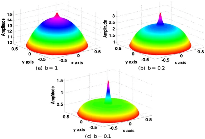
We have introduced a thresholdκ to shift the zero of the Heaviside function. We make the assumption that the system is spatially homogeneous that is, the external inputI does not depend upon the variablest and the connectivity function depends only on the hyperbolic distance between two points ofD: W (z, z)=W (d2(z, z)). For illustrative purposes, we will use the exponential weight distribution as a specific example throughout this section:
W (z, z)=Wd2(z, z)
=exp
−d2(z, z)
b
. (21)
The theoretical study of equation (20) has been done in [21] where the authors have imposed strong regularity assumptions on the kernel function W, such as Hölder continuity, and used compactness arguments and integral equation techniques to ob-tain a global existence result of solutions to (20). Our approach is very different, we follow that of [25–29,31] by proceeding in a constructive fashion. In a first part, we define what we call a hyperbolic radially symmetric bump and present some pre-liminary results for the linear stability analysis of the last part. The second part is devoted to the proof of a technical Theorem5.1.1which is stated in the first part. The proof uses results on the Fourier transform introduced in Section4, hyperbolic ge-ometry and hypergeometric functions. Our results will be illustrated in the following Section6.
5.1 Existence of hyperbolic radially symmetric bumps
From equation (20) a general stationary pulse satisfies the equation:
αV (z)=
{z∈D|V (z)≥κ}
W (z, z)dm(z)+Iext(z).
For convenience, we noteM(z, K)the integral KW (z, z)dm(z)withK= {z∈
Definition 5.1.1 V is called a hyperbolic radially symmetric stationary-pulse solu-tion of(20)ifV depends only upon the variablerand is such that:
V (r) > κ, r∈ [0, ω[,
V (ω)=κ,
V (r) < κ, r∈ ]ω,∞[, V (∞)=0,
and is a fixed point of equation(20):
αV (r)=M(r, ω)+Iext(r), (22)
whereIext(r)=Ie− r2
2σ2 is a Gaussian input andM(r, ω)is defined by the following equation:
M(r, ω)def=Mz, Bh(0, ω)
andBh(0, ω)is a hyperbolic disk centered at the origin of hyperbolic radiusω.
From symmetry arguments there exists a hyperbolic radially symmetric stationary-pulse solutionV (r) of (20), furthermore the threshold κ and width ω are related according to the self-consistency condition
ακ=M(ω)+Iext(ω)
def
=N (ω), (23)
where
M(ω)def=M(ω, ω).
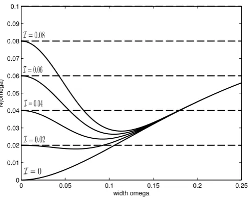
The existence of such a bump can then be established by finding solutions to (23) The functionN (ω)is plotted in Figure1for a range of the input amplitudeI. The horizontal dashed lines indicate different values ofακ, the points of intersection de-termine the existence of stationary pulse solutions. Qualitatively, for sufficiently large input amplitudeI we have N(0) <0 and it is possible to find only one solution branch for largeακ. For small input amplitudesI we haveN(0) >0 and there al-ways exists one solution branch forαβ < γc≈0.06. For intermediate values of the
input amplitudeI, asαβvaries, we have the possiblity of zero, one or two solutions. Anticipating the stability results of Section5.3, we obtain that whenN(ω) <0 then the corresponding solution is stable.
We end this subsection with the usefull and technical following formula.
Theorem 5.1.1 For all(r, ω)∈R+×R+:
M(r, ω)=1
4sinh(ω) 2
cosh(ω)2
R
W(λ)(λ0,0)(r)(λ1,1)(ω)λtanh
π
2λ
Fig. 1 Plot ofN (ω)defined in (23) as a function of the pulse widthωfor several values of the input amplitudeIand for a fixed input widthσ=0.05. The horizontal dashed lines indicate different values of
ακ. The connectivity function is given in equation (21) and the parameterbis set tob=0.2.
whereW(λ)is the Fourier Helgason transform ofW(z)def=W (d2(z,0))and
(α,β)λ (ω)=F
1
2(ρ+iλ), 1
2(ρ−iλ);α+1; −sinh(ω) 2
,
withα+β+1=ρandF is the hypergeometric function of first kind.
Remark 5.1.1 We recall thatF admits the integral representation[32]:
F (α, β;γ;z)= (α)
(β)(γ−β)
1 0
tβ−1(1−t )γ−β−1(1−t z)−αdt
with(γ ) >(β) >0.
Remark 5.1.2 In Section4we introduced the functionλ(z)=∂De(iλ+1)z,bdb. In[22],it is shown that:
(λ0,0)(r)=λ
tanh(r) if z=tanh(r)eiθ.
Remark 5.1.3 Let us point out that this result can be linked to the work of Folias and Bressloff in[31]and then used in[29].They constructed a two-dimensional pulse for a general,radially symmetric synaptic weight function.They obtain a similar formal representation of the integral of the connectivity functionw over the diskB(O, a)
centered at the originOand of radiusa.Using their notations,
M(a, r)=
2π
0
a
0
w|r−r|r dr dθ=2π a
∞
0
˘
whereJν(x)is the Bessel function of the first kind andw˘ is the real Fourier transform
ofw.In our case,instead of the Bessel function,we find(ν,ν)λ (r)which is linked to the hypergeometric function of the first kind.
We now show that for a general monotonically decreasing weight functionW, the functionM(r, ω)is necessarily a monotonically decreasing function ofr. This will ensure that the hyperbolic radially symmetric stationary-pulse solution (22) is also a monotonically decreasing function ofr in the case of a Gaussian input. The demonstration of this result will directly use Theorem5.1.1.
Proposition 5.1.1 V is a monotonically decreasing function inrfor any monotoni-cally decreasing synaptic weight functionW.
Proof DifferentiatingMwith respect toryields:
∂M
∂r (r, ω)=
1 2
ω
0
2π
0
∂ ∂r
Wd2
tanh(r),tanh(r )eiθsinh(2r) dr dθ.
We have to compute
∂ ∂r
Wd2
tanh(r),tanh(r)eiθ
=W d2
tanh(r),tanh(r)eiθ∂ ∂r
d2
tanh(r),tanh(r)eiθ.
It is result of elementary hyperbolic trigonometry that
d2
tanh(r),tanh(r )eiθ
=tanh−1
tanh(r)2+tanh(r)2−2 tanh(r)tanh(r )cos(θ ) 1+tanh(r)2tanh(r)2−2 tanh(r)tanh(r)cos(θ )
(25)
we letρ=tanh(r),ρ =tanh(r)and define
Fρ,θ(ρ)=
ρ2+ρ2−2ρρ cos(θ )
1+ρ2ρ2−2ρρ cos(θ ). It follows that
∂
∂ρtanh
−1F
ρ,θ(ρ)
=
∂
∂ρFρ,θ(ρ)
2(1−Fρ,θ(ρ))
Fρ,θ(ρ) ,
and
∂
∂ρFρ,θ(ρ)=
2(ρ−ρ cos(θ ))+2ρρ(ρ −ρcos(θ )) (1+ρ2ρ2−2ρρ cos(θ ))2 . We conclude that ifρ >tanh(ω)then for all 0≤ρ ≤tanh(ω)and 0≤θ≤2π
which impliesM(r, ω) <0 forr > ω, sinceW <0.
To see that it is also negative forr < ω, we differentiate equation (24) with respect tor:
∂M
∂r (r, ω)=
1 4sinh(ω)
2
cosh(ω)2
×
R
W(λ) ∂
∂r
(0,0)
λ (r)
(1,1)
λ (ω)λtanh
π
2λ
dλ.
The following formula holds for the hypergeometric function (see Erdelyi in [32]):
d
dzF (a, b;c;z)= ab
c F (a+1, b+1;c+1;z).
It implies
∂
∂r
(0,0)
λ (r)= −
1
2sinh(r)cosh(r)
1+λ2(λ1,1)(r).
Substituting in the previous equation giving ∂∂rMwe find:
∂M
∂r (r, ω)= −
1
64sinh(2ω) 2
sinh(2r)
×
R
W(λ)1+λ2λ(1,1)(r)(λ1,1)(ω)λtanh
π
2λ
dλ,
implying that:
sgn
∂M
∂r (r, ω)
=sgn
∂M
∂r (ω, r)
.
Consequently, ∂∂rM(r, ω) <0 forr < ω. HenceV is monotonically decreasing inr
for any monotonically decreasing synaptic weight functionW.
As a consequence, for our particular choice of exponential weight function (21), the radially symmetric bump is monotonically decreasing inr, as it will be recover in our numerical experiments in Section6.
5.2 Proof of Theorem5.1.1
The proof of Theorem5.1.1goes in four steps. First we introduce some notations and recall some basic properties of the Fourier transform in the Poincaré disk. Second we prove two propositions. Third we state a technical lemma on hypergeometric func-tions, the proof being given in LemmaF.0.4of AppendixF. The last step is devoted to the conclusion of the proof.
5.2.1 First step
Proposition 5.2.1 For all(r, ω)∈R+×R+:
M(r, ω)= 1
4π
R
W(λ)λ∗1Bh(0,ω)(z)λtanh
π
2λ
dλ. (26)
Proof We start with the definition ofM(r, ω)and use the convolutional form of the integral:
M(r, ω)=Mz, Bh(0, ω)
=
Bh(0,ω)
W (z, z)dm(z)
=
DW (z, z)1Bh(0,ω)(z)dm(z)=W∗1Bh(0,ω)(z).
In [22], Helgason proves an inversion formula for the hyperbolic Fourier transform and we apply this result toW:
W(z)= 1
4π R ∂D
W(λ, b)e(iλ+1)z,bλtanh
π 2λ dλ db = 1 4π R W(λ) ∂D
e(iλ+1)z,bdb
λtanh π 2λ dλ
the last equality is a direct application of Lemma4.2.1and we can deduce that
W(z)= 1
4π
R
W(λ)λ(z)λtanh
π
2λ
dλ. (27)
Finally we have:
M(r, ω)=W∗1Bh(0,ω)(z)= 1 4π
R
W(λ)λ∗1Bh(0,ω)(z)λtanh
π
2λ
dλ.
which is the desired formula.
It appears that the study ofM(r, ω)consists in calculating the convolution product
λ∗1Bh(0,ω)(z).
Proposition 5.2.2 For allz=k·Ofork∈G=SU(1,1)we have:
λ∗1Bh(0,ω)(z)=
Bh(0,ω)
λk−1·zdm(z).
Proof Letz=k·Ofork∈Gwe have:
λ∗1Bh(0,ω)(z)=
G
1Bh(0,ω)(g·O)λ
g−1·zdg
=
G
1Bh(0,ω)(g·O)λ